Session Types Revisited

HAL Id: hal-01647086

https://hal.inria.fr/hal-01647086

Submitted on 26 Nov 2017

HAL is a multi-disciplinary open access

archive for the deposit and dissemination of

sci-entific research documents, whether they are

pub-lished or not. The documents may come from

L’archive ouverte pluridisciplinaire HAL, est

destinée au dépôt et à la diffusion de documents

scientifiques de niveau recherche, publiés ou non,

émanant des établissements d’enseignement et de

Session Types Revisited

Ornela Dardha, Elena Giachino, Davide Sangiorgi

To cite this version:

Ornela Dardha, Elena Giachino, Davide Sangiorgi. Session Types Revisited. Information and

Com-putation, Elsevier, 2017, 256, pp.253 - 286. �10.1016/j.ic.2017.06.002�. �hal-01647086�

Session Types Revisited

Ornela Dardhaa, Elena Giachinob, Davide Sangiorgib

a_{School of Computing Science, University of Glasgow, United Kingdom} b_{INRIA Focus Team / DISI, University of Bologna, Italy}

Abstract

Session types are a formalism used to model structured communication-based programming. A binary session type describes communication by specifying the type and direction of data exchanged between two parties. When session types and session processes are added to the syntax of standard π-calculus they give rise to additional separate syntactic categories. As a consequence, when new type features are added, there is duplication of effort in the theory: the proofs of properties must be checked both on standard types and on session types. We show that session types are encodable into standard π-types, relying on linear and variant types. Besides being an expressivity result, the encoding (i) removes the above redundancies in the syntax, and (ii) the properties of session types are derived as straightforward corollaries, exploiting the corresponding properties of standard π-types. The robustness of the encoding is tested on a few extensions of session types, including subtyping, polymorphism and higher-order communications.

Keywords: session types, π-calculus, linear types, variant types, encoding.

1. Introduction

In complex distributed systems, participants willing to communicate should previously agree on a protocol to follow. The specified protocol describes the types of messages that are exchanged as well as their direction. In this context session types [15, 28, 16] came into play: they describe a protocol as a type ab-straction. Session types were originally designed for process calculi. However, they have been studied also for other paradigms, such as multi-threaded func-tional programming [31], component-based systems [29], object-oriented lan-guages [10, 11, 3], Web Services and Contracts, W3C-CDL a language for chore-ography [5, 21] and many more. Session types are a type formalism proposed as a theoretical foundation to describe and model structured communication-based programming, guaranteeing properties like session fidelity, privacy and communication safety.

Email addresses: Ornela.Dardha@glasgow.ac.uk (Ornela Dardha),

Session types are defined as a sequence of input and output operations, ex-plicitly indicating the types of messages being transmitted. This structured sequentiality of operations is what makes session types suitable to model pro-tocols. However, they offer more flexibility than just performing inputs and outputs: they also permit internal and external choice. Branch and select are typical type (and term) constructs in the theory of session types, the former being the offering of a set of alternatives and the latter being the selection of one of the possible options at hand.

As mentioned above, session types guarantee session fidelity, privacy and communication safety. Session fidelity guarantees that the session channel has the expected structure. Privacy is guaranteed since session channels are known and used only by the participants involved in the communication. Such com-munication proceeds without any mismatch of direction and of message type. In order to achieve communication safety, a session channel is split by giving rise to two opposite endpoints, each of which is owned by one of the partici-pants. These endpoints are used according to dual behaviours and thus have dual types, namely one participant sends what the other one is expecting to receive and vice versa. So, duality is a key concept in the theory of session types as it is the ingredient that guarantees communication safety.

To better understand session types and the notion of duality, let us consider a simple example: the equality test. A client and a server communicate over a session channel. The endpoints x and y of the session channel are owned by the client and the server respectively and exclusively and must have dual types. To guarantee duality of types, static checks are performed by the type system. If the type of x is

?Int.?Int.!Bool.end

— meaning that the process listening on channel endpoint x receives (?) an integer value followed by another integer value and then sends (!) back a boolean value corresponding to the equality test of the integers received — then the type of y should be

!Int.!Int.?Bool.end

— meaning that the process listening on channel endpoint y sends an integer value followed by another integer value and then waits to receive back a boolean value — which is exactly the dual type.

There is a precise moment at which a session between two participants is established. It is the connection phase, when a fresh (private) session channel is created and its endpoints are bound to each communicating process. The con-nection is also the moment when duality, hence compliance of two session types, is verified. In order to establish a connection, primitives like accept/request

or(νxy), are added to the syntax of terms [28, 16, 30].

Session types and session terms are added to the syntax of standard π-calculus types and terms, respectively. In doing so, the syntax of types often needs to be split into two separate syntactic categories, one for session types and the other for standard π-calculus types [28, 16, 33, 14] (this often intro-duces a duplication of type environments, as well). Common typing features,

like subtyping, polymorphism, recursion are then added to both syntactic

cat-egories. Also the syntax of processes will contain both standard π-calculus

process constructs and session process constructs (for example, the constructs mentioned above to create session channels). This redundancy in the syntax brings in redundancy also in the theory, and can make the proofs of properties of the language heavy. In particular, this duplication becomes more obvious in proofs by structural induction on types. Moreover, if a new type construct is added, the corresponding properties must be checked both on standard π-types and on session types. By “standard type systems” we mean type systems orig-inally studied in depth in sequential languages such as the λ-calculus and then transplanted onto the π-calculus as types for channel names (rather than types for terms as in the λ-calculus). Such type systems may include constructs for products, records, variants, polymorphism, linearity, and so on.

In this paper we aim to understand to which extent this redundancy is necessary, in the light of the following similarities between session constructs and standard π-calculus constructs. Consider ?Int.?Int.!Bool.end. This type is assigned to a session channel endpoint and it describes a structured sequence of inputs and outputs by specifying the type of messages that it can transmit. This way of proceeding reminds us of the linearised channels [20], which are channels used multiple times for communication but only in a sequential manner. This paper [20] discusses the possibility of encoding linearised channel types into linear types—i.e., channel types used exactly once.

The considerations above deal with input and output operations and the se-quentiality of session types. Let us consider branch and select. These constructs give more flexibility by offering and selecting a range of possibilities. This brings in mind an already existing type construct in the π-calculus, namely the variant type [26, 27]. Another analogy between the session types theory and the stan-dard π-types theory, concerns duality. As mentioned above, duality is checked when connection takes place, in the typing rule for channel restriction. Duality describes the split of behaviour of session channel endpoints. This reminds us of the split of input and output capabilities of π-types: once a new channel is created via the ν construct, it can then be used by the two communicating processes owning the opposite capabilities.

In this paper, by following Kobayashi’s approach [19], we define an encoding of binary session types into standard π-types and by exploiting this encoding, session types and their theory are shown to be derivable from the theory of the standard typed π-calculus. For instance, basic properties such as subject reduction and type safety become straightforward corollaries. Intuitively, a ses-sion type is interpreted as a linear channel type carrying a pair consisting of the original payload type and a new linear channel type, which is going to be used for the continuation of the communication. Furthermore, we present an optimisation of linear channels enabling the reuse of the same channel, instead of a new one, for the continuation of the communication. As stated above, the encoding we adopt follows Kobayashi [19] and the constructs we use are not new (linear types and variant types are well-known concepts in type theory and they are also well integrated in the π-calculus). Indeed the technical

contribu-tion of the paper may be considered minor (the main technical novelty being the optimisation in linear channel usage mentioned above). Rather than tech-nical, the contribution of the paper is meant to be foundational: we show that Kobayashi’s encoding

(i) does permit to derive session types and their basic properties; and (ii) is a robust encoding.

As evidence for (ii), in this paper we examine, besides plain session types, a few extensions of them, such as subtyping, polymorphism and higher-order features in Sections 4, 5 and 6, respectively. These are non-trivial extensions, which have been studied in dedicated session types papers [14, 12, 22]. In each case we show that we can derive the main results of these papers via the encoding, as straightforward corollaries. As long as the encoding is concerned, these exten-sions follow the same line as the encoding of types and terms given in Section 3. We will avoid repeating technical results, when it is not necessary. Hence, Sections 4, 5 and 6 are less detailed than Section 3. While Kobayashi’s encoding was generally known, its strength, robustness, and practical impact were not. This is witnessed by the plethora of papers on session types over the last 20 years, in which session types are always taken as primitives — we are not aware of a single work that explains the results on session types via an encoding of them into standard types. In our opinion, the reasons why Kobayashi’s encoding had not caught attention are:

(a) Kobayashi did not prove any properties of the encoding and did not in-vestigate its robustness;

(b) as certain key features of session types do not clearly show up in the encoding, the faithfulness of the encoding was unclear.

A good example for (b) is duality. In session types theory, duality plays a central role: a session is identified by two channel endpoints, and these must have dual types. In the standard typed π-calculus, in contrast, there is no notion of duality on types. Indeed, in the encoding, dual session types (e.g., the branch type and the select type) are mapped onto the same type (e.g., the variant type). In general, dual session types will be mapped onto linear types that are identical except for the outermost I/O tag — duality on session types boils down to the opposite input and output capabilities of channels.

The results in the paper are not however meant to imply that session types are useless, as they are very useful from a programming perspective. The work just tells us that, at least for the binary sessions and properties examined in the paper, session types and session primitives may be taken as macros. This paper is an extension of the conference version [8] and further details can be found in the first author’s published Ph.D. thesis [7].

Structure: The remainder of the paper is structured as follows. Section 2 gives an overview of session types and standard π-calculus types as well as

language terms, typing rules and operational semantics. Section 3 presents

the encoding of both session types and session processes. Sections 4, 5 and 6 present extensions of session types: subtyping, polymorphism and higher-order

T ∶∶= S (session type)

♯ T (channel type)

Unit (unit type)

. . . (other constructs)

S∶∶= end (termination)

?T.S (receive)

!T.S (send)

&{li∶ Si}i∈I (branch)

⊕{li∶ Si}i∈I (select)

P, Q∶∶= x!⟨v⟩.P (output) 0 (inaction)

x?(y).P (input) P ∣ Q (composition)

x◁ lj.P (selection) (νxy)P (session restriction)

x▷ {li∶ Pi}i∈I (branching) (νx)P (channel restriction)

v∶∶= x (name) ⋆ (unit value)

Figure 1: Syntax of the π-calculus with session types

communication, respectively and analyse the encoding with respect to these extensions. Section 7 presents an optimisation of linear channel usage. Section 8 examines related work and Section 9 concludes the paper.

2. Background

In this section we give an overview of the two theories we will be working with: session types theory and standard typed π-calculus theory.

2.1. Session Types

Type Syntax. Types are presented at the top of Fig. 1. The syntax of types is given by two separate syntactic categories: one for session types and the other for standard π-types, which includes session types. We use S to range over session types and T to range over types. Session types are: end, the type of a terminated session endpoint; ?T.S and !T.S indicating, respectively a session type assigned to an endpoint used to receive and to send a value of type T and then continue according to the protocol specified by session type S. Branch and select are sets of labelled session types, where the order of components does not matter and labels are all distinct. The labelled components of branch and

select range over an index set I. Branch &{li∶ Si}i∈I indicates external choice,

namely what is offered, and it is a generalisation of the input type. Dually,

select⊕{li∶ Si}i∈I indicates the internal choice, only one of the labels will be

chosen, and it is a generalisation of the output type. Types T include session

types, standard channel types ♯ T , Unit type and if required other standard

π-type constructs, such as other ground types like Int, String, . . ., or classes, data types etc.

Language Syntax. The syntax of terms is presented at the bottom of Fig. 1 and it follows [30]. There are different ways of presenting session channel initiation and endpoints, like accept/request [16], polarised channels [14] or by means of co-names [30]. Standard communication (not involving sessions) is based on standard π-calculus channels [16, 14], whereas in [30] it is based on co-names. In this paper we use co-names for session communication and standard π-calculus channels otherwise. Co-names specify the two opposite endpoints of a communication channel and are created and bound together by the restriction construct. Our results can be applied to all the different syntaxes in session types theory.

We use P, Q to range over processes, x, y over names and v to range over values. We use fn(P ) to denote the set of free names in P , bn(P ) to denote the bound ones and n(P ) = fn(P ) ∪ bn(P ) to denote the set of all names in P . We adopt the Barendregt name convention, namely that all names in bindings in any mathematical context are pairwise distinct and distinct from the free names.

The output process x!⟨v⟩.P sends a value v on x and proceeds as process P ; the

input process x?(y).P receives on x a value to substitute the placeholder y in

the continuation process P . The selection process x◁ lj.P on x selects label lj

and proceeds as process P . The branching process x▷ {li∶ Pi}i∈I on x offers a

range of alternatives each labelled with a different label ranging over the index

set I. According to the selected label lj the process Pj will be executed. The

process 0 is the standard inaction process. The last two constructs represent

restriction. (νxy)P is the session restriction construct; it creates a session

channel, more precisely its two endpoints x and y and binds them in P . The two endpoints should be distinguished to validate subject reduction (see [33]).

The type system enforces duality of behaviours on endpoints. Process(νx)P is

the standard channel restriction; it creates a new channel x and binds it with scope P .

Duality. Two processes willing to communicate, e.g., a client and a server, must first agree on a protocol. The protocol is abstracted as a structured type, namely a session type. Intuitively, client and server should perform dual operations: when one process sends, the other receives, when one offers, the other chooses. So, the dual of an input is an output, the dual of branch is select, and vice versa. Formally, duality on session types is defined as:

end ≜ end

!T.S ≜ ?T.S

?T.S ≜ !T.S

⊕{li∶ Si}i∈I ≜ &{li∶ Si}i∈I

&{li∶ Si}i∈I ≜ ⊕{li∶ Si}i∈I

In order to guarantee that communication is safe and proceeds without any mismatch, static checks are performed by the type system. These checks control that the opposite endpoints of the same session channel have dual types, as we will see shortly.

∅ = ∅ ○ ∅ Γ= Γ1○ Γ2 un(T ) Γ, x∶ T = (Γ1, x∶ T ) ○ (Γ2, x∶ T ) Γ= Γ1○ Γ2 lin(S) Γ, x∶ S = (Γ1, x∶ S) ○ Γ2 Γ= Γ1○ Γ2 lin(S) Γ, x∶ S = Γ1○ (Γ2, x∶ S)

Figure 2: Context split for session types

Typing Rules. A typing context Γ is a partial function from names to types. We

use dom(Γ) to denote the domain of Γ. Typing judgements for values are of the

form Γ⊢ v ∶ T , reading “a value v is of type T in a typing context Γ”. Typing

judgements for processes are of the form Γ⊢ P , reading “a process P is well

typed in a typing context Γ”. In order to deal with linearity, the typing rules make use of lin and un predicates and a context split operator ‘○’. The lin and un predicates state when a type, or a typing context, is linear or unrestricted, respectively [30].

lin(T ) if T is a session type and T≠ end

un(T ) otherwise

lin(Γ) if there is(x ∶ T ) ∈ Γ such that lin(T )

un(Γ) otherwise

The context split ‘○’ is defined by the rules in Fig. 2. Intuitively, these rules

state that a typing context is split in a way that linear names occur only in one of the halves. This does not hold for the unrestricted names.

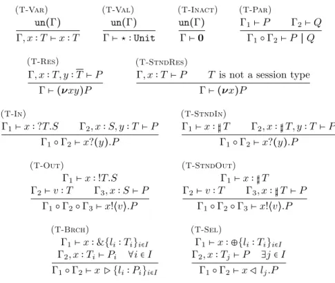
The typing rules for the π-calculus with session types are given in Fig. 3.

Rule (T-Var) states that a name x is of type T , if this is the type assumed in

the typing context. Rule (T-Val) states that a unit value is of unit type. Rule

(T-Inact) states that the terminated process 0 is always well typed under any Γ.

Notice that in all the previous rules, the typing context Γ is unrestricted. Rule (T-Par) types the parallel composition of two processes under the combination

of typing contexts by using the split operator. The rule that performs duality

checks is the rule for session restriction (T-Res). Process(νxy)P is well typed

in Γ, if P is well typed in Γ augmented with session channel endpoints having

dual types, namely x∶ T and y ∶ T . Rule (T-In) splits in two the context in

which the input process x?(y).P is well typed: one part typechecks x, the other

part augmented with y∶ T and updated with x ∶ S, typechecks the continuation

process P . The rule for output (T-Out) is similar. The context is split in three

parts, one to typecheck x, another to typecheck v and the last part to typecheck the continuation process P . Similarly to the input rule, the continuation process uses channel x with its continuation type S. In addition to the typing rules for session restriction, input and output, there are also the corresponding ones for

standard channel types, namely the typing rules (T-StndRes), (T-StndIn) and

(StndOut). This is an example of the duplication of rules and work that is

(T-Var) un(Γ) Γ, x∶ T ⊢ x ∶ T (T-Val) un(Γ) Γ⊢ ⋆ ∶ Unit (T-Inact) un(Γ) Γ⊢ 0 (T-Par) Γ1⊢ P Γ2⊢ Q Γ1○ Γ2⊢ P ∣ Q (T-Res) Γ, x∶ T, y ∶ T ⊢ P Γ⊢ (νxy)P (T-StndRes)

Γ, x∶ T ⊢ P T is not a session type

Γ⊢ (νx)P (T-In) Γ1⊢ x ∶ ?T.S Γ2, x∶ S, y ∶ T ⊢ P Γ1○ Γ2⊢ x?(y).P (T-StndIn) Γ1⊢ x ∶ ♯ T Γ2, x∶ ♯ T, y ∶ T ⊢ P Γ1○ Γ2⊢ x?(y).P (T-Out) Γ1⊢ x ∶ !T.S Γ2⊢ v ∶ T Γ3, x∶ S ⊢ P Γ1○ Γ2○ Γ3⊢ x!⟨v⟩.P (T-StndOut) Γ1⊢ x ∶ ♯ T Γ2⊢ v ∶ T Γ3, x∶ ♯ T ⊢ P Γ1○ Γ2○ Γ3⊢ x!⟨v⟩.P (T-Brch) Γ1⊢ x ∶ &{li∶ Ti}i∈I Γ2, x∶ Ti⊢ Pi ∀i ∈ I Γ1○ Γ2⊢ x ▷ {li∶ Pi}i∈I (T-Sel) Γ1⊢ x ∶ ⊕{li∶ Ti}i∈I Γ2, x∶ Tj⊢ P ∃j ∈ I Γ1○ Γ2⊢ x ◁ lj.P

Figure 3: Typing rules for the π-calculus with session types

the typing rules (T-Brch) and (T-Sel). The branching process x▷ {li∶ Pi}i∈I is

well typed if channel x is of branch type &{li ∶ Ti}i∈I and every continuation

process Pi is well typed and uses x with type Ti. To typecheck a process that

selects label lj on channel x of type⊕{li∶ Ti}i∈I, we typecheck the continuation

process Pj that uses x with type Tj.

Operational Semantics. The operational semantics is defined as a binary

rela-tion→ over processes and is given in Fig. 4. Rule (R-StndCom) is the standard

communication rule. In rule (R-Com), two processes communicate on two

co-names, and the value so received replaces the input placeholder. Rule (R-Case) is

similar: the communicating processes have prefixes that are co-names, and the

label received selects the continuation on the recipient side. Rules (R-StndRes),

(R-Res), (R-Par), and (R-Struct) are standard, stating that communication can

happen under restriction and parallel composition and allowing to exploit the structural congruence relation.

(R- StndCom) x!⟨v⟩.P ∣ x?(z).Q → P ∣ Q[v/z]

(R-Com) (νxy)(x!⟨v⟩.P ∣ y?(z).Q) → (νxy)(P ∣ Q[v/z])

(R-Case) (νxy)(x ◁ lj.P ∣ y ▷ {li∶ Pi}i∈I) → (νxy)(P ∣ Pj) j ∈ I

(R-StndRes) P→ Q Ô⇒ (νx)P → (νx)Q

(R-Res) P→ Q Ô⇒ (νxy)P → (νxy)Q

(R-Par) P→ Q Ô⇒ P ∣ R → Q ∣ R

(R-Struct) P≡ P′, P → Q, Q′≡ Q Ô⇒ P′→ Q′ Figure 4: Semantics for the π-calculus with session types

P ∣ Q ≡ Q ∣ P (P ∣ Q) ∣ R ≡ P ∣ (Q ∣ R) P ∣ 0 ≡ P (νxy)0 ≡ 0 (νx)0 ≡ 0 (νxy)(νzw)P ≡ (νzw)(νxy)P (νx)P ∣ Q ≡ (νx)(P ∣ Q) (x ∉ fn(Q)) (νxy)(νzw)P ≡ (νzw)(νxy)P (νxy)P ∣ Q ≡ (νxy)(P ∣ Q) (x, y ∉ fn(Q))

In order to complete the operational semantics, structural congruence relation,

denoted as ≡, is needed and is defined as the smallest congruence relation on

processes that satisfies the above axioms. The first three axioms state that parallel composition of processes is commutative, associative and uses process 0 as the neutral element. The remaining axioms involve restriction, the main ones being scope extrusion stating that the scope of a restriction can be extended to other processes in parallel provided that no capture of (session co-) names occurs. To conclude, let C, D range over contexts. Intuitively, a context is a process with a hole [27].

Properties. We recall some basic properties of the session π-calculus [30]. The weakening lemma states that it is sound to introduce unrestricted type assump-tions in a typing context.

Lemma 1 (Weakening in Sessions). If Γ⊢ P and x ∉ fn(P ) and un(T ), then

Γ, x∶ T ⊢ P .

The strengthening lemma states somehow the opposite of weakening: it is sound to remove unrestricted names from the typing context provided that they do not occur free in the process being typed.

Lemma 2 (Strengthening in Sessions). If Γ, x ∶ T ⊢ P and x ∉ fn(P ) and

τ∶∶= `_o[̃τ] (linear output) _♯[̃τ] (connection)

`_i[̃τ] (linear input) ⟨li τi⟩i∈I (variant type)

`♯[̃τ] (linear connection) Unit (unit type)

∅[] (no capability) . . . (other constructs)

P, Q∶∶= x!⟨˜v⟩.P (output) 0 (inaction)

x?(˜y).P (input) P ∣ Q (composition)

(νx)P (restriction) case v of{li (xi) ▷ Pi}i∈I (case)

v∶∶= x (name) ⋆ (unit value)

l v (variant value)

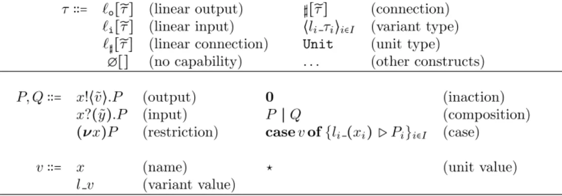
Figure 5: Syntax of the standard typed π-calculus

We are ready now to state the subject congruence and the subject reduction properties for the session π-calculus.

Lemma 3 (Subject Congruence for Sessions). If Γ⊢ P and P ≡ P′_{, then Γ}⊢ P′_.

Theorem 4 (Subject Reduction for Sessions). If Γ⊢ P and P → Q, then Γ ⊢ Q.

2.2. π-Types

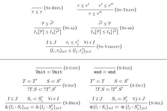
Type Syntax. We now consider the standard typed π-calculus [27]. The syntax of the type constructs is presented at the top of Fig. 5. The standard π-types, ranged over by τ , include various type constructs. Here we focus on linear types and variant types, which will be used in the encoding. We use a tilde

˜ to indicate a sequence of elements. Linear types `i[̃τ], `o[̃τ] and `♯[̃τ] are

assigned to channels used exactly once in input to receive messages of typẽτ,

in output to send messages of typẽτ and used once for sending and once for

receiving messages of typẽτ, respectively. The type ∅[] is assigned to a channel

without any capability. We use α, β to range over the i, o or♯ capabilities. Type

♯[̃τ] indicates a channel used for communication without any restriction. The

variant type ⟨li τi⟩i∈I is a labelled form of disjoint union of types. The order

of the components does not matter and labels are all distinct. Unit type is standard. Other type constructs, like ground types and recursive types, can be added to the syntax.

We define a notion of duality on π-types to be the duality on the capability of the channel, via the following rules:

`i[̃τ] = `o[̃τ]

`o[̃τ] = `i[̃τ]

∅[] = ∅[]

Language Syntax. The syntax of terms of the π-calculus is given at the bottom

(Γ1⊎ Γ2)(x) ≜ ⎧⎪⎪⎪ ⎪⎪⎪⎪ ⎨⎪⎪ ⎪⎪⎪⎪⎪ ⎩

Γ1(x) ⊎ Γ2(x) if both Γ1(x) and Γ2(x) are defined

Γ1(x) if Γ1(x), but not Γ2(x), is defined

Γ2(x) if Γ2(x), but not Γ1(x), is defined

undef otherwise

Figure 6: Context combination for linear π-types

and proceeds as P ; input process x?(˜y).P receives on x a tuple of values that

is going to substitute ˜y in P ; restriction process (νx)P creates a new name x

and binds it with scope P ; differently from session π-calculus, here we have only one restriction process. Inaction and parallel composition are standard. Process

case v of{li (xi)▷Pi}i∈Ioffers different behaviours depending on which variant

value l v it receives. Values include names, variant values and the unit value. Typing Rules. The predicates lin and un on the standard π-types and typing contexts are defined as:

lin(τ) if τ= `α[̃τ] or (τ = ⟨li τi⟩i∈I and for some j∈ I. lin(τj))

un(τ) otherwise

lin(Γ) if there is(x ∶ τ) ∈ Γ such that lin(τ)

un(Γ) otherwise

As for session types, also for linear types there is a careful handling of typing

contexts in order to ensure linearity. The combination ‘⊎’ of types is a symmetric

operation and is defined by the following rules, and the combination of typing contexts is defined in Fig. 2.2.

`i[̃τ] ⊎ `o[̃τ] ≜ `♯[̃τ]

τ⊎ τ ≜ τ if un(τ)

τ⊎ τ′ ≜ undef _otherwise

Typing judgements for the standard typed π-calculus have the same shape as the corresponding ones for the session typed π-calculus. The typing rules are

given in Fig. 7. Rule (Tπ-Var) states that a name has type the one assumed

in the typing context. Rule (Tπ-Val) states that a unit value has type Unit.

Both rules use an unrestricted typing context. Rule (Tπ-Inact) states that the

terminated process 0 is well typed in every unrestricted typing context. Rule (Tπ-Par) states that the parallel composition of two processes is well typed in

the combination of typing contexts used to type each of the processes. There

are two typing rules for the restriction process(νx)P . Rule (Tπ-Res1) states

that the restriction process(νx)P is well typed if process P is well typed under

the same typing context augmented with x∶ `♯[̃τ]. By applying the definition of

context combination given in Fig. 2.2, we have x∶ `♯[̃τ] = x ∶ `i[̃τ] ⊎ `o[̃τ]. This

(Tπ-Var) un(Γ) Γ, x∶ τ ⊢ x ∶ τ (Tπ-Val) un(Γ) Γ⊢ ⋆ ∶ Unit (Tπ-Inact) un(Γ) Γ⊢ 0 (Tπ-Par) Γ1⊢ P Γ2⊢ Q Γ1⊎ Γ2⊢ P ∣ Q (Tπ-Res1) Γ, x∶ `♯[̃τ] ⊢ P Γ⊢ (νx)P (Tπ-Res2) Γ, x∶ ∅[] ⊢ P Γ⊢ (νx)P (Tπ-Inp) Γ1⊢ x ∶ `i[̃τ] Γ2, ˜y∶ ̃τ ⊢ P Γ1⊎ Γ2⊢ x?(˜y).P (Tπ-Out) Γ1⊢ x ∶ `o[̃τ] ̃Γ2⊢ ˜v ∶ ̃τ Γ3⊢ P Γ1⊎ ̃Γ2⊎ Γ3⊢ x!⟨˜v⟩.P (Tπ-LVal) Γ⊢ v ∶ τj j∈ I Γ⊢ lj v∶ ⟨li τi⟩i∈I (Tπ-Case) Γ1⊢ v ∶ ⟨li τi⟩i∈I Γ2, xi∶ τi⊢ Pi ∀i ∈ I Γ1⊎ Γ2⊢ case v of {li (xi) ▷ Pi}i∈I

Figure 7: Typing rules for the standard typed π-calculus

(Rπ-Com) x!⟨˜v⟩.P ∣ x?(˜z).Q → P ∣ Q[˜v/˜z]

(Rπ-Case) case lj v of{li (xi) ▷ Pi}i∈I→ Pj[v/xj] j ∈ I

(Rπ-Res) P → Q Ô⇒ (νx)P → (νx)Q

(Rπ-Par) P → Q Ô⇒ P ∣ R → Q ∣ R

(Rπ-Struct) P ≡ P′, P → Q, Q′≡ Q Ô⇒ P′→ Q′ Figure 8: Semantics for the standard typed π-calculus

This is a fundamental feature used in the encoding. Rule (Tπ-Res2) states that

(νx)P is well typed if P is well typed and x has no capabilities in P . This rule is needed in the standard typed π-calculus to prove subject reduction (see [27]),

and it is needed also for our encoding. Rules (Tπ-Inp) and (Tπ-Out) state that

the input and output processes are well typed if x is a linear channel used in input and output, respectively and the carried types are compatible with the

types of ˜y and ˜v, respectively We use ̃Γ to denote Γ1⊎. . . ⊎Γksuch that k is the

length of the sequence denoted bỹ⋅. A variant value lj v is of type⟨li τi⟩i∈I if

v is of type τj for j∈ I. Process case v of {li (xi) ▷ Pi}i∈I is well typed if value

v has variant type and every process Pi is well typed assuming xi has type τi.

Operational Semantics. The semantics of the π-calculus is presented in Fig. 8.

Rule (Rπ-Com) is very similar to the corresponding one in session processes.

The only difference here is that we are considering the polyadic π-calculus.

Rule (Rπ-Case) is also called a case normalisation. The case process reduces to

(Rπ-Par) state that communication and case normalisation can happen under

restriction and parallel composition, respectively. Rule (Rπ-Struct) states that

reduction can happen under structural congruence ≡, which is defined in the

same way as in the previous section for session π-calculus semantics; the only difference being that there are no rules for co-names.

Properties. We recall some basic properties of the type system with linear π-types [27]. They follow the same intuition as the analogous properties for session types given in the previous section.

Definition 5 (Closed Typing Context). A typing context is closed if for all

x∈ dom(Γ), then Γ(x) ≠ `♯[̃τ].

Lemma 6 (Substitution Lemma for Linear π-calculus). Let Γ, x∶ τ ⊢ P , and

let Γ⊎ Γ′_{be defined and Γ}′⊢ v ∶ τ. Then, Γ ⊎ Γ′⊢ P [v/x].

Lemma 7 (Weakening in Linear π-calculus). If Γ⊢ P and x ∉ fn(P ) and un(τ),

then Γ, x∶ τ ⊢ P .

Lemma 8 (Strengthening in Linear π-calculus). If Γ, x∶ τ ⊢ P and x ∉ fn(P )

and un(τ), then Γ ⊢ P .

We are ready now to state the subject congruence and the subject reduction properties for the linear π-calculus.

Lemma 9 (Subject Congruence for Linear π-calculus). If Γ⊢ P and P ≡ P′_,

then Γ⊢ P′_.

Theorem 10 (Subject Reduction for Linear π-calculus). If Γ⊢ P with Γ closed

and P→ P′_{, then Γ}⊢ P′_.

By analysing and combining the definition of closed typing context with the statement of the subject reduction property for linear π-calculus, we notice that since the typing context has no linear channel owning both capabilities

(condi-tion≠ `♯[̃τ]), if a process reduces it is either the result of a case normalisation

or of a communication on a restricted channel owning both capabilities of input and output. The reason for adopting a closed typing context is to avoid reduc-tions of typing contexts due to reducreduc-tions of processes. This gives a simpler statement of the subject reduction property. Further details can be found in Sangiorgi and Walker [27].

We conclude the section with a lemma showing that if two structurally con-gruent processes reduce by consuming exactly the same prefixes, then the deriva-tives are again structurally congruent. To express this, we use a marking of the involved prefixes, as a way of pointing out the specific prefixes involved (we mark only a prefix, not the process underneath it). The marking does not otherwise affect syntax and operational semantics.

Lemma 11. Suppose P has exactly one input and one output prefix that are

prefixes are consumed. Suppose also that P ≡ Q and that Q → Q′ _{in which,}

as before, precisely the two marked input and output prefixes are consumed.

Then, also P′≡ Q′_.

Proof. Straightforward proof on the number of axioms of structural congruence

applied to infer P≡ Q.

3. Encoding

Session types guarantee that only the communicating parties know the cor-responding endpoints of the session channel, thus providing privacy. Moreover, the opposite endpoints should have dual types, thus providing communication safety. The interpretation of session types should take into account these fun-damental issues. In order to guarantee privacy and safety of communication we adopt linear channels, which are used exactly once. Privacy is ensured since the linear channel is known only to the interacting parties. Communication safety is ensured by the type safety of linear types. Furthermore, in order to preserve the structure of a session type and the session fidelity property, our encoding is based on the continuation-passing principle.

3.1. Type Encoding

We present the encoding of session types into linear π-types at the top of

Fig. 9. All the other types are encoded in a homomorphic way, namely_{J♯ TK ≜}

♯JT K and JUnitK ≜ Unit. The encoding of end is a channel with no capabilities, meaning that it cannot be used neither for input nor for output. Type ?T.S is interpreted as the linear input channel type carrying a pair of values whose types are the encoding of T and of S. The encoding of !T.S is similar. However, in this case it is the dual of S to be sent since it is the type of a channel as used by the receiver. This will be shown later by an example of the encoding. The branch and the select types are generalisations of input and output types, respectively. Consequently, they are interpreted as linear input and linear output channels

carrying variant types having the same labels li and, as types respectively, the

encoding of Si and of Si for all i∈ I. Again, the reason for duality is the same

as for the output type. 3.2. Process Encoding

The encoding of session processes into π-calculus processes is defined at the bottom of Fig. 9. The encoding of terms differs from the encoding of types as it is parametrised by a function, ranging over f, g, from names to names. We use

dom(f) to denote the domain of function f. We use fx, fy as an abbreviation

for f(x), f(y), respectively.

Let P be a session process. We say that a function f is a renaming function

for P , if for all names x∈ fn(P ), the image fxis either x, or it is a fresh name

not included in n(P ); and f is the identity function on all bound names of P .

JendK ≜ ∅[] (E-End)

J!T .S K ≜ `o[JT K, JS K] (E-Out)

J?T .S K ≜ `i[JT K, JS K] (E-Inp)

J⊕{li∶ Si}i∈IK ≜ `o[⟨li JSiK⟩i∈I] (E-Select)

J&{li∶ Si}i∈IK ≜ `i[⟨li JSiK⟩i∈I] (E-Branch)

JxKf ≜ fx (E-Name)

J⋆Kf ≜ ⋆ (E-Star)

J0Kf ≜ 0 (E-Inaction)

Jx!⟨v⟩.P Kf ≜ (νc)fx!⟨JvKf, c⟩.JP Kf,{x↦c} (E-Output)

Jx?(y).P Kf ≜ fx?(y, c).JP Kf,{x↦c} (E-Input)

Jx ◁ lj.PKf ≜ (νc)fx!⟨lj c⟩.JP Kf,{x↦c} (E-Selection)

Jx ▷ {li∶ Pi}i∈IKf ≜ fx?(y). case y of {li (c) ▷JPiKf,{x↦c}}i∈I (E-Branching)

JP ∣ QKf ≜ JP Kf ∣ JQKf (E-Composition)

J(ν xy)P Kf ≜ (νc)JP Kf,{x,y↦c} (E-Restriction)

Figure 9: Encoding of types and terms

as in f,{x ↦ c} or f, {x, y ↦ c}, where names x and y are now associated to c,

namely f(x) and f(y) are updated to c. The notion of a renaming function is

extended also to values, being ground values and names, as expected. In the uses of the definition of renaming function f for P (respectively v), process P (respectively value v) will be typed in a typing context, say Γ. We will implicitly

assume that the fresh names used by f (that is, the names y such that y= f(x),

for some x≠ y) are also fresh for Γ (that is, they are not in dom(Γ). We prefer

to avoid the explicit mention of the typing context Γ so to ease the reading of the statements.

We explain now the reason for f . Since we are using linear channels, once a channel is used, it cannot be used again for transmission. To enable structured communications however, like session types do, the channel is renamed: a new channel is created and is sent to the partner in order to use it to continue the rest of the session. This procedure is repeated at every step of communication and the function f is updated to the new name created. This is the continuation-passing principle.

We provide some explanations on the encoding. A channel name x is encoded by using a renaming function f for x, meaning that f is defined on x. The encoding of the unit value is the unit value itself. This holds for every ground value added to the language. In the encoding of the output process, a new channel name c is created and is sent together with the encoding of the payload v

along the channel fx; the encoding of the continuation process P is parametrised

fx and receives a value, that substitutes name y and a fresh channel c that

substitutes x in the continuation process encoded in f updated with{x ↦ c}.

As indicated in Section 2.1, session restriction(νxy)P creates two fresh names

and binds them in P as being the opposite endpoints of the same session channel.

This is not needed in the standard π-calculus. The restriction construct(νx)P

creates and binds a unique name x to P ; this name identifies both endpoints of the communicating channel. The encoding of a session restriction process

(νxy)P is a linear channel restriction process (νc)JP Kf,{x,y↦c} with the new

name c used to substitute x and y in the encoding of P . The last two constructs

correspond to selection and branching processes. Selection x◁ lj.P is encoded

as the process that first creates a new channel c and then sends on fxa variant

value lj c, where lj is the selected label and c is the channel created to be used

for the continuation of the session. The encoding of branching receives on fx a

value, typically being a variant value, which is the guard of the case process.

According to the chosen label, one of the corresponding processes_JPiKf,{x↦c}for

i∈ I, will be chosen. Note that the name c is bound in any process_JPiKf,{x→c}.

The encoding of the other process constructs, like inaction, standard scope

restriction, and parallel composition, is a homomorphism, namely _J0Kf ≜ 0,

J(ν x)P Kf≜ (νx)JP Kf, andJP ∣ QKf≜JP Kf ∣JQKf.

3.3. Example: the Mathematical Server and Client

In this section we present an example of a mathematical server and a client communicating with it, from Gay and Hole [14]; the example illustrates channel interaction as well as branching and selection. We assume ground types like Int, Bool and standard mathematical operations on ground values. We present the encoding of types and processes, and the operational semantics of both the session system and its encoding. The server offers three mathematical operations as services: addition of integers; the equality test; and negation of integers. The server runs in parallel with a client, which selects among the services offered. Communication occurs along a session channel with endpoints x for the server and y for the client.

The session type S for the server endpoint x is defined as:

S ≜ &{ plus ∶ ?Int.?Int.!Int.end,

equal∶ ?Int.?Int.!Bool.end,

neg∶ ?Int.!Int.end }

The session type for the client endpoint y must be dual to S and is thus defined as:

S ≜ ⊕{ plus ∶ !Int.!Int.?Int.end,

equal∶ !Int.!Int.?Bool.end,

Now we move to processes. The server process is defined as:

server ≜ x ▷ { plus ∶ x?(v1).x?(v2).x!⟨v1+ v2⟩.0,

equal∶ x?(v1).x?(v2).x!⟨v1== v2⟩.0,

neg∶ x?(v).x!⟨−v⟩.0 }

We have x∶ S ⊢ server. The client must be typechecked by using S. By rule

(T-Sel) this means that the client chooses one of the possible branches specified

in its type. Thus, a possible client is:

client ≜ y ◁ equal.y!⟨3⟩.y!⟨5⟩.y?(eq).0

Such a client selects the equality test, which we already mentioned in the in-troduction. The client sends to the server two integers 3 and 5, and waits for a boolean answer. Once all this is done, both processes terminate. The whole system is given by

(νxy)(server ∣ client) which, as outlined above, reduces thus:

(νxy)(server ∣ client) → (νxy)(x?(v1).x?(v2).x!⟨v1== v2⟩.0 ∣ y!⟨3⟩.y!⟨5⟩.y?(eq).0)

→ (νxy)(x?(v2).x!⟨3 == v2⟩.0 ∣ y!⟨5⟩.y?(eq).0)

→ (νxy)(x!⟨3 == 5⟩.0 ∣ y?(eq).0) → 0

We are ready now to present the encoding of the system. We start with session types. We have:

JS K = `i[⟨ plus `i[Int, `i[Int, `o[Int, ∅[]]]]

equal `i[Int, `i[Int, `o[Bool, ∅[]]]],

neg `i[Int, `o[Int, ∅[]]] ⟩]

(1)

and

JS K = `o[⟨ plus `i[Int, `i[Int, `o[Int, ∅[]]]]

equal `i[Int, `i[Int, `o[Bool, ∅[]]]],

neg `<sub>i</sub>[Int, `_o[Int, ∅[]]] ⟩]

(2)

When examining (1) and (2) we notice that duality on session types boils down

to opposite capabilities of linear channel types. Indeed the encodings _{JS K and}

JS K only differ in the capabilities of the outermost linear types `i[⋅] and `o[⋅].

Thus checking the duality between two session types amounts to checking, in the encoding, this simple duality on capabilities.

Now we move to processes. When encoding processes, the initial renaming

function is the identity function, below simply indicated as∅:

J(ν xy)(server ∣ client)K∅ = (νz)J(server ∣ client)K{x,y↦z}

where JserverK{x↦z} = z?(y).case y of { plus(s) ▷ s?(v1, c).c?(v2, c′).(νc′′)c′!⟨v1+ v2, c′′⟩.0 equal(s) ▷ s?(v1, c).c?(v2, c′).(νc′′)c′!⟨v1== v2, c′′⟩.0 neg (s) ▷ s?(v, c).(νc′′)c!⟨−v, c′′⟩.0 } and

JclientK{y↦z} = (νs)z!⟨equal s⟩.(νc)s!⟨3, c⟩.(νc

′)c!⟨5, c′⟩.c′_?(eq, c′′).0

The renaming function{x, y ↦ z} maps the session endpoints x and y to a fresh

name z; after that, in every output of the session, a new channel is created and sent to the partner together with the payload. For example, the client creates and sends a name s together with the selected label equal, and afterwards it

creates the channels c, c′_{and c}′′_{, for the rest of the communication. Note that,}

when a new channel is created, for example in(νc), it has both the input and

the output capabilities. The client process sends to the server, at channel s, the payload 3 and the input capability of the new channel c, retaining for itself the output capability. Interaction then continues along such new channel c, with the sending of the payload 5 and the output capability of a new continuation

channel c′_{. Here is how the encoded system evolves:}

(νz)(JserverKf,{x↦z} ∣JclientKf,{y↦z})

→ (νs)(case equal s of {. . .} ∣ (νc)s!⟨3, c⟩.(νc′)c!⟨5, c′⟩.c′ ?(eq, c′′).0) → (νs)(s?(v1, c).c?(v2, c′).(νc′′)c′!⟨v1== v2, c′′⟩.0 ∣ (νc)s!⟨3, c⟩.(νc′)c!⟨5, c′⟩.c′ ?(eq, c′′).0) →∗(νc′′)c′_!⟨3 == 5, c′′⟩.0 ∣ c′_?(eq, c′′).0 → 0

The first reduction of the encoded maths system corresponds to the first re-duction of the original system, where a label (namely equal ) is selected. The second reduction is a case normalisation, where a pattern matching of the case guard occurs so to identify the appropriate continuation process. The case nor-malisation is the only reduction in the encoded system that does not have a corresponding reduction in the original system; it represents however an ad-ministrative reduction, without a real computational content. The remaining reductions of the encoded systems, which for simplicity have not been detailed, are in one-to-one correspondence with the reductions of the original system. 3.4. Properties of the Encoding

The encoding previously presented can be considered as the semantics of session types and session terms. The following results show that indeed we can derive the typing judgements and the properties of the π-calculus with sessions

J∅Kf ≜ ∅ (E-Empty)

JΓ, x ∶ T Kf ≜ JΓKf⊎ fx∶JT K (E-Gamma)

Figure 10: Encoding of typing contexts

via the encoding and the corresponding typing judgements and properties in the standard π-calculus.

In order to prove these results, we need to extend the encoding to session typing contexts. Given a session process P , respectively a value v, such that

there is a session typing context Γ with Γ⊢ P , respectively Γ ⊢ v ∶ T , and a

renaming function f for P , respectively v, we use f in the encoding of Γ as defined in Fig. 10.

3.4.1. Auxiliary Results

We start this section with some auxiliary results. The following proposition states that the encoding of typing contexts, given in Fig. 10, is sound and complete with respect to predicates lin and un.

Proposition 12. Let Γ be a session typing context and q be either lin or un.

Then q(Γ) if and only if q(JΓKf), for all renaming functions f for Γ.

The following two lemmas give the relation between the combination

oper-ator ‘⊎’ and the standard ‘,’ operator in linear π-typing contexts.

Lemma 13. If Γ, x∶ T is defined, then also Γ ⊎ x ∶ T is defined.

Proof. By definition of ‘,’ on typing contexts, it means that x ∉ dom(Γ). We

conclude by definition of combination of typing contexts.

Lemma 14. If Γ⊎ x ∶ T is defined and x ∉ dom(Γ), then also Γ, x ∶ T is defined.

Proof. Immediate by definition of combination of typing contexts.

The following two lemmas give a relation between the context split operator

‘○’ used in session typing contexts and the combination operator ‘⊎’ used in

linear π-typing contexts by using the encoding of typing contexts presented in Fig. 10.

Lemma 15 (Split to Combination). Let Γ1, . . . , Γn be session typing contexts

such that Γ1○ . . . ○ Γn is defined, then

JΓ1○ . . . ○ ΓnKf =JΓ1Kf⊎ . . . ⊎JΓnKf

for some renaming function f for Γ1○ . . . ○ Γn.

Proof. It follows immediately by the definitions of the encoding on typing con-texts, given in Fig. 10, and the combination on typing concon-texts, given in Fig. 2.2.

Lemma 16 (Combination to Split). Let Γ be a session typing context and f

a renaming function for Γ and_JΓKf = Γπ1 ⊎ . . . ⊎ Γ

π

n. Then, for all i∈ {1 . . . n},

there exist Γi such thatJΓiKf= Γ

π

i and Γ1○ . . . ○ Γn= Γ.

Proof. It follows immediately by the encoding of typing contexts given in Fig. 10

and Fig. 2 on context split ‘○’ for session types.

The following lemma relates the encoding of dual session types with dual linear π-types.

Lemma 17 (Encoding of Dual Session Types). If_{JT K = τ then JT K = τ .}

Proof. The proof is by induction on the structure of the session type T . We use the duality of session types defined in Section 2.1 and the duality of standard π-types defined in Section 2.2.

• T = end

By (E-End) we haveJendK = ∅[] and T = end. We conclude by the duality

of∅[].

• T = !T.U

By (E-Out) we haveJ!T .U K = `o[JT K, JU K]. By the duality of session types

we have !T.U = ?T.U. By (T-In) we have J?T .U K = `i[JT K, JU K]. We

conclude by the duality of π-types. • T = ?T.U

By (E-In) we have J?T .U K = `i[JT K, JU K]. By the duality of session types

we have ?T.U = !T.U. By (E-Out) we have J!T .U K = `o[JT K, JU K], which

by the involution property of duality on session types is `o[JT K, JU K]. We

conclude by the duality of π-types.

• T = ⊕{li∶ Ti}i∈I

By (E-Select) we haveJ⊕{li∶ Ti}i∈IK = `o[⟨li JTiK⟩i∈I] By duality on session

types we have⊕{li∶ Ti}i∈I= &{li∶ Ti}i∈I. By (E-Branch) we haveJ&{li∶

Ti}i∈IK = `i[⟨li JTiK⟩i∈I] We conclude by the duality of π-types.

• T = &{li∶ Ti}i∈I

By (E-Branch) we haveJ&{li∶ Ti}i∈IK = `i[⟨li JTiK⟩i∈I] By duality on

ses-sion types we have &{li∶ Ti}i∈I = ⊕{li ∶ Ti}i∈I. By (E-Select) we have

J⊕{li∶ Ti}i∈IK = `o[⟨li JTiK⟩i∈I], which by the involution property of

dual-ity on session types means `_o[⟨li JTiK⟩i∈I]. We conclude by the duality of

π-types.

3.4.2. Type Correctness for Values

We state the soundness and completeness of the encoding in typing deriva-tions for values. The correctness of an encoded typing judgement on the target terms implies the correctness of the judgement on the source terms, and con-versely.

Lemma 18 (Soundness). If_JΓKf ⊢JvKf ∶JT K for some renaming function f for

v, then Γ⊢ v ∶ T .

Proof. The proof is done by induction on the structure of the value v: • Case v = x:

By (E-Name) we have JxKf = fx and assume JΓKf ⊢ fx ∶ JT K. By rule (Tπ-Var) it means that (fx ∶JT K) ∈ JΓKf. Hence, (x ∶ T

′) ∈ Γ for some type T′_{. By (} E-Gamma) it must be JT ′ K = JT K which implies T ′= T . By

Proposition 12 also un(Γ1) holds. By applying rule (T-Var) we obtain the

result. • Case v = ⋆:

By (E-Star) we have J⋆Kf = ⋆ and assumeJΓKf ⊢ ⋆ ∶ Unit and un(JΓKf).

Then un(Γ) holds by Proposition 12. We conclude by rule (T-Val).

Lemma 19 (Completeness). If Γ ⊢ v ∶ T , then _JΓKf ⊢ JvKf ∶ JT K for some

renaming function f for v.

Proof. The proof is done by induction on the derivation Γ⊢ v ∶ T .

• Case (T-Var):

un(Γ)

Γ, x∶ T ⊢ x ∶ T

By (E-Gamma) and (E-Name) we haveJΓKf⊎fx∶JT K ⊢ fx∶JT K. We conclude

by Proposition 12, Lemma 14 and typing rule (Tπ-Var).

• Case (T-Val):

un(Γ)

Γ⊢ ⋆ ∶ Unit

Follows immediately from the encoding of⋆ and Unit, Proposition 12 and

rule (Tπ-Val).

3.4.3. Type Correctness for Processes

We state the soundness and completeness of the encoding in typing deriva-tions for processes.

Theorem 20 (Soundness). If_JΓKf⊢JP Kf for some renaming function f for P ,

then Γ⊢ P .

Proof. The proof is by induction on the structure of session process P . We only present some of the cases.

• Case 0:

By (E-Inaction) we have J0Kf = 0 and assume JΓKf ⊢ 0, where un(JΓKf) holds. By Proposition 12 also un(Γ) holds. We conclude by applying

• Case P ∣ Q: By (E-Composition) we have JP ∣ QKf = JP Kf ∣ JQKf and

assume_JΓKf⊢JP Kf ∣JQKf, which by rule (Tπ-Par) means:

Γπ₁ ⊢_{JP K}f Γπ2 ⊢JQKf Γπ₁⊎ Γπ₂ ⊢_{JP K}f ∣JQKf where _JΓKf = Γπ1 ⊎ Γ π 2. By Lemma 16 Γ π 1 =JΓ1Kf and Γ π 2 =JΓ2Kf, such

that Γ= Γ1○ Γ2. By induction hypothesis we have Γ1⊢ P and Γ2⊢ Q. By

applying (T-Par) we obtain the result Γ1○ Γ2⊢ P ∣ Q.

• Case x?(y).P :

By (E-Input) we haveJx?(y).P Kf = fx?(y, c).JP Kf,{x↦c}and assumeJΓKf⊢

fx?(y, c).JP Kf,{x↦c} which by rule (Tπ-Inp) means:

Γπ1 ⊢ fx∶ `i[T π , Sπ] Γπ2, c∶ S π , y∶ Tπ⊢_{JP K}f,{x↦c} JΓKf⊢ fx?(y, c).JP Kf,{x↦c}

where _JΓKf = Γπ1 ⊎ Γπ2. By Lemma 16 Γπ1 =JΓ1Kf and Γ

π

2 =JΓ2Kf, with

Γ= Γ1○Γ2. By Lemma 18 we have Γ1⊢ x ∶ ?T.S. By induction hypothesis

Γ2, x∶ S, y ∶ T ⊢ P where Tπ=JT K, S

π ₌

JS K and the renaming function

f,{x ↦ c} is used in the encoding of P . By applying (T-Inp) we obtain

Γ1○ Γ2⊢ x?(y).P .

Theorem 21 (Completeness). If Γ⊢ P , then _JΓKf ⊢JP Kf for some renaming

function f for P .

Proof. The proof is by induction on the derivation Γ⊢ P . We present the main

cases.

• Case (T-Res):

Γ, x∶ T, y ∶ T ⊢ P

(T-Res)

Γ⊢ (νxy)P

Notice that x, y∉ dom(Γ) by typability assumptions. We distinguish the

following two cases:

– Suppose T ≠ end. By duality on session types also T ≠ end. By

induction hypothesis we have _{JΓ, x ∶ T , y ∶ T K}f′ ⊢

JP Kf′, for some

renaming function f′_{for P , which by (}

E-Gamma) means thatJΓKf′⊎ f′

x∶JT K ⊎ f

′

y ∶JT K ⊢ JP Kf′. Let f = f

′ _{and update f with}{x, y ↦ c}

for a fresh name c that does not occur in the codomain of f . We

will use f,{x, y ↦ c} as a renaming function. By Lemma 17, _{JT K = τ}

and _{JT K = τ .} Since T ≠ end and T ≠ end, we have _{JT K = `}α[W ]

and _{JT K = `}α[W ] and by the combination of linear channel types

`α[W ] ⊎ `α[W ] = `♯[W ], where W denotes the pair of carried types,

induction hypothesis as_JΓKf⊎c ∶ `♯[W ] ⊢JP Kf,{x,y↦c}. By Lemma 14

we obtain _JΓKf, c∶ `♯[W ] ⊢JP Kf,{x,y↦c}. By applying (Tπ-Res1) we

obtain_JΓKf⊢ (νc)JP Kf,{x,y↦c}, which concludes this case.

– Suppose T = end. By duality on session types also T = end. By

induction hypothesis we have_{JΓ, x ∶ end, y ∶ endK}f′⊢

JP Kf′, for some

renaming function f′_{for P . By (}

E-Gamma) it means thatJΓKf′⊎ f

′ x∶

JendK ⊎ f

′

y∶JendK ⊢ JP Kf′. Let f = f

′_{and update f with}{x, y ↦ c} for

a fresh name c that does not occur in the codomain of f . We will now

use f,{x, y ↦ c} as a renaming function for P . Hence, we can rewrite

the induction hypothesis as _JΓKf ⊎ c ∶ ∅[] ⊎ c ∶ ∅[] ⊢ JP Kf,{x,y↦c},

which by the combination of unrestricted types meansJΓKf⊎c ∶ ∅[] ⊢

JP Kf,{x,y↦c}. Moreover, c∉ dom(JΓKf), since c is chosen fresh, then

by Lemma 14 we obtain_JΓKf, c∶ ∅[] ⊢JP Kf,{x,y↦c}. We conclude by

rule (Tπ-Res2).

• Case (T-Brch):

Γ1⊢ x ∶ &{li∶ Ti}i∈I Γ2, x∶ Ti⊢ Pi ∀i ∈ I

(T-Brch)

Γ1○ Γ2⊢ x ▷ {li∶ Pi}i∈I

By applying Lemma 19 we have that _JΓ1Kf′ ⊢ Jx ∶ &{li ∶ Ti}i∈IKf′, for

some renaming function f′_{for x, which by (}

E-Branch) means thatJΓ1Kf′⊢ f′

x ∶ `i[⟨li JTiK⟩i∈I]. By induction hypothesis and by (E-Gamma) we have

that JΓ2Kf′′⊎ f_x′′ ∶ _{JTiK ⊢ JPiKf}′′ for some renaming function f′′ for P_i,

for all i ∈ I. Since Γ1○ Γ2 is defined, by definition of context split, for

all x ∈ dom(Γ1) ∩ dom(Γ2) it holds that Γ1(x) = Γ2(x) = T and un(T ).

Let dom(Γ1) ∩ dom(Γ2) = D and define fD′ = f

′∖ ⋃

d∈D{d ↦ f′(d)} and

f′′ D= f

′′

∖ ⋃d∈D{d ↦ f′′(d)}. Suppose f′′(x) = c. Then, let f = ⋃d∈D{d ↦

d′} ∪ f′ D∪ f

′′

D∖ {x ↦ c}, where for all d ∈ D we create a fresh name d

′_and

map d to d′_{. Moreover, f is a function since its subcomponents act on}

disjoint domains. Then, by applying Lemma 6, the above can be rewritten as:

JΓ1Kf ⊢ fx∶ `i[⟨li JTiK⟩i∈I] JΓ2Kf⊎ c ∶JTiK ⊢ JPiKf,{x↦c} for all i∈ I

Since x ∉ dom(Γ2), then JΓ2, x ∶ TiKf,{x↦c} can be distributed and thus

optimised as_JΓ2Kf⊎c ∶JTiK. By rules (Tπ-Case), and (Tπ-Var) for deriving

y∶ ⟨li JTiK⟩i∈I, and Lemma 14 we have the following derivation:

(Tπ-Case) (Tπ-Var)

y∶ ⟨li JTiK⟩i∈I⊢ y ∶ ⟨li JTiK⟩i∈I

JΓ2Kf, c∶JTiK ⊢ JPiKf,{x↦c} ∀i ∈ I

JΓ2Kf, y∶ ⟨li JTiK⟩i∈I⊢ case y of {li (c) ▷JPiKf,{x↦c}}i∈I

(Tπ-Inp)

JΓ1Kf⊢ fx∶ `i[⟨li JTiK⟩i∈I]

JΓ2Kf, y∶ ⟨li JTiK⟩i∈I⊢ case y of {li (c) ▷JPiKf,{x↦c}}i∈I

JΓ1Kf⊎JΓ2Kf⊢ fx?(y). case y of {li (c) ▷JPiKf,{x↦c}}i∈I

By applying (E-Branching) and Lemma 15 we conclude this case.

3.4.4. Operational Correspondence

In this section we prove the operational correspondence. This property states that the encoding of processes is sound and complete with respect to the oper-ational semantics of the π-calculus with and without sessions.

We start with a lemma which relates the encoding of processes and name substitution.

Lemma 22. Let P be a session process and let P[v/z] denote process P where

name z is substituted by value v. Then,

JP [v/z]Kf = JP Kf[JvKf/f(z)]

for all renaming functions f for P and v in which, for all names x, we have

f(x) = z if and only if x = z.

Proof. It follows immediately from the encoding of processes given in Fig. 9.

Lemma 23 (Structural Congruence and Encoding). Let P and P′ _{be session}

processes. Then, P ≡ P′ _{if and only if}

JP Kf ≡JP

′

Kf for all renaming functions

f for P and P′_.

Proof. The proof is done by induction on the number of axioms of structural congruence applied.

Let↪ denote ≡ extended with a case normalisation, namely a reduction by

using (Rπ-Case). We are ready now to formally state the operational

correspon-dence.

Theorem 24 (Operational Correspondence). Let P be a session process, Γ a

session typing context, and f a renaming function for P such that_JΓKf ⊢JP Kf.

Then the following statements hold.

1. If P→ P′_{, then}

JP Kf →↪JP

′

Kf.

2. If_{JP K}f→ Q, then there is a session process P′such that

• either P → P′_;

• or there are x, y such that (νxy)P → P′

and Q↪_JP′

Kf.

Proof. Notice that, since_JΓKf⊢JP Kf, by Theorem 20 it means that Γ⊢ P . We

prove separately the two assertions of the theorem.

• Case (R-Com):

P ≜ (νxy)(x!⟨v⟩.Q1 ∣ y?(z).Q2) → (νxy)(Q1 ∣ Q2[v/z]) ≜ P′

By the encoding of output and input processes we have:

JP Kf = J(ν xy)(x!⟨v⟩.Q1 ∣ y?(z).Q2)Kf

= (νc) (Jx!⟨v⟩.Q1 ∣ y?(z).Q2Kf,{x,y↦c})

= (νc) (Jx!⟨v⟩.Q1Kf,{x,y↦c} ∣Jy?(z).Q2Kf,{x,y↦c})

= (νc) ((νc′)(c!⟨JvK f, c′⟩.JQ1Kf,{x,y↦c,x↦c′_}) ∣ c?(z, c ′).JQ 2Kf,{x,y↦c,y↦c′_}) → (νc) ((νc′)(JQ 1Kf,{x,y↦c,x↦c′_} ∣_{JQ2Kf,{x,y↦c,y↦c}′_}[JvK_f/z])) ≡ (νc′)(JQ 1Kf,{x,y↦c,x↦c′_} ∣_{JQ2Kf,{x,y↦c,y↦c}′_}[JvK_f/z])

Since P is a session-typed process, it means x∉ fn(Q2) and y ∉ fn(Q1).

Then, both f,{x, y ↦ c, x ↦ c′} and f, {x, y ↦ c, y ↦ c′} can be replaced

by f,{x, y ↦ c′}. We can rewrite the above as:

(νc′)(JQ

1Kf,{x,y↦c′_} ∣_{JQ2Kf,{x,y↦c}′_}[JvK_f/z])

Since z is bound with scope Q2 it means that fz= z. The encoding of P′

using f as a renaming function is as follows: JP ′ Kf = J(ν xy)(Q1 ∣ Q2[v/z])Kf = (νc′)(JQ 1Kf,{x,y↦c′_} ∣_JQ2[v/z]K_f,{x,y↦c′_}) = (νc′)(JQ

1Kf,{x,y↦c′_} ∣_{JQ2Kf,{x,y↦c}′_}[JvK_f,{x,y↦c′_}/JzK_f,{x,y↦c′_}])

= (νc′)(JQ

1Kf,{x,y↦c′} ∣JQ2Kf,{x,y↦c′}[JvKf/fz])

= (νc′)(JQ

1Kf,{x,y↦c′_} ∣_JQ2Kf,{x,y↦c′_}[JvKf/z])

In order to obtain_JQ2Kf,{x,y↦c′_}[JvK_f,{x,y↦c′_}/JzK_f,{x,y↦c′_}] above, we use

Lemma 22. Function f coincides with f,{x, y ↦ c′} when applied to value

v and fz= z, so we obtainJQ2Kf,{x,y↦c′_}[JvK_f/z]; meaning:

JP Kf →≡JP

′

Kf

• Case (R-Sel):

By the encoding of selection and branching processes we have:

JP Kf = J(ν xy)(x ◁ lj.Q∣ y ▷ {li∶ Pi}i∈I)Kf

= (νc) (Jx ◁ lj.Q∣ y ▷ {li∶ Pi}i∈IKf,{x,y↦c})

= (νc) (Jx ◁ lj.QKf,{x,y↦c} ∣ Jy ▷ {li∶ Pi}i∈IKf,{x,y↦c})

= (νc) ((νc′)(c!⟨l

j c′⟩.JQKf,{x,y↦c,x↦c′_}) ∣

c?(z).case z of {li (c′) ▷JPiKf,{x,y↦c,y↦c′_}}i∈I)

→ (νc) ((νc′)(JQK

f,{x,y↦c,x↦c′_}∣

case lj c′of{li (c′) ▷JPiKf,{x,y↦c,y↦c′_}}_i∈I))

→ (νc) ((νc′)(JQK

f,{x,y↦c,x↦c′_}∣

JPjKf,{x,y↦c,y↦c′}))

≡ (νc′)(JQK

f,{x,y↦c,x↦c′_} ∣_JPjKf,{x,y↦c,y↦c′_})

Since P is well typed, it means that for all i∈ I, x ∉ fn(Pi) and y ∉ fn(Q).

Then, both f,{x, y ↦ c, x ↦ c′} and f, {x, y ↦ c, y ↦ c′} can be replaced

by f,{x, y ↦ c′}. We can rewrite the above as:

(νc′)(JQK

f,{x,y↦c′_}∣ _{JPjKf,{x,y↦c}′_}) On the other hand we have:

JP ′ Kf = J(ν xy)(Q ∣ Pj)Kf = (νc′)(JQK f,{x,y↦c′_}∣ JPjKf,{x,y↦c′})

The above implies:

JP Kf →↪JP ′ Kf • Case (R-Par): P → Q P ∣ R → Q ∣ R

By (E-Composition) we haveJP ∣ RKf=JP Kf ∣JRKf. By induction

hypoth-esis JP Kf →↪ JQKf. We conclude that JP Kf ∣ JRKf →↪JQKf ∣ JRKf by

applying (Rπ-Par) and (Rπ-Struct).

• Case (R-Struct): P≡ P′ , P′→ Q′ , Q′≡ Q P → Q By induction hypothesis_JP′ Kf →↪JQ ′

Kf, and f is a renaming function for

P′_{. By Lemma 23 we have} JP Kf ≡JP ′ Kf andJQ ′ Kf ≡JQKf. We conclude by (Rπ-Struct).

2. We discuss the case in which the reduction_{JP K}f → Q is due to an

endpoints. The case of unrestricted names, as well as the case in which the reduction originates from the case construct are simpler, and are handled along the same line.

The input and the output prefixes that are consumed in the reductionJP Kf →

Q must be top-level, in the sense that they are not underneath other prefixes. To identify such prefixes, we suppose they are marked (in the same way as we did in Lemma 11).

Consider now the corresponding input and output prefixes in the session pro-cess P (those that produce, via the encoding, the two marked input and output

prefixes of_{JP K}f). Using structural congruence we can obtain a process R≡ P

in which such prefixes are in contiguous position. Precisely, using structural congruence we can make sure that R is of the form:

R= C[ x!⟨v⟩.P1 ∣ y?(z).P2]

where x!⟨v⟩.P1and y?(z).P2are the mentioned input and output processes and

the hole of the context is at top level.

Since R ≡ P , it is sufficient to prove the statement of the theorem for R

in place of P , as any derivative of R is also a derivative of P . Moreover, by Lemma 23, we also have that

JP Kf ≡ JRKf

where_JRKf is of the form

JRKf= D[Jx!⟨v⟩.P1Kg ∣Jy?(z).P2Kg] (3)

for some context D[⋅] with a top-level hole, and some renaming function g with

g(x) = g(y). Now, expanding the definition of the encoding, for some fresh

name c, and using brackets for the marked prefixes, we can continue from (3) as follows:

= D[ (νc)gx!⟨JvKg, c⟩.JP1Kg,{x↦c} ∣ gy?(z, c).JP2Kg,{y↦c}]

→ D[ (νc)(JP1Kg,{x↦c} ∣JP2Kg,{y↦c}[JvKg/z]) ] ≜ Q

′ ₍₄₎

Appealing to Lemma 11, we know that such a reduction, having consumed the two marked prefixes yields the following equivalence:

Q′≡ Q

We will now find the derivative P′_{of the assertion of theorem (as a derivative}

of R) and prove

Q′≡

JP

′

Kf

For this we distinguish two cases, corresponding to the cases in the statement of the theorem:

(i) x and y are not restricted in R (that is (νxy) does not appear in the

(ii) x and y are restricted session endpoints, namely co-names.

The distinction is relevant because, in the π-calculus with sessions, communi-cations along session endpoints is only possible if such endpoints are co-names.

We consider the second case (ii) first. Since (νxy) appears in the context

C[⋅], its encoded context D[⋅] contains a restriction (νc′) where c′_{is the linear}

name g(x) (and also g(y)). The reduction in (4) is along the name c′_{, which,}

being linear, after the reduction does not occur anymore in the continuation process. We can therefore remove such a restriction and simply replace it with

the restriction at c. If E[⋅] is the context with c′ _{replaced by c, we therefore}

have the following:

Q′≡ E[

JP1Kg,{x↦c}∣ JP2Kg,{y↦c}[JvKg/z] ] ≜ Q ′′

Moreover, since(νxy) is in the context C[⋅], we can infer the reduction:

R= C[ x!⟨v⟩.P1∣ y?(z).P2] → C[ P1∣ P2[v/z] ] ≜ P′ (5)

We can show that Q′′=

JP ′ Kf as follows: JP ′ Kf = D[JP1Kg ∣ JP2[v/z]Kg] = D[JP1Kg ∣ JP2Kg[JvKg/z] ]

where we have applied Lemma 22, and then, by renaming c′ _{into c, namely by}

using context E[⋅], we obtain Q′′_.

Now the case (i), which is simpler. In this case context D[⋅] does not contain

a restriction on c′_{; indeed name c}′ _{does not appear in Q}′_{. As} (νxy) is not in

C[⋅], to infer a reduction akin to (5) we have to add (νxy) as follows:

(νxy)R = (νxy)C[ x!⟨v⟩.P1 ∣ y?(z).P2] → (νxy)C[ P1 ∣ P2[v/z] ]

≡ C[ (νxy)(P1 ∣ P2[v/z]) ] ≜ P′

Then, one concludes Q′=

JP

′

Kf.

Note that the statement of item 2 of the operational correspondence theorem

uses↪. In case the reduction of the session process P is due to an input and

output communication, as in the proof outlined above, then ↪ is simply ≡.

Otherwise, in case the reduction of the session process P is due to a branching

and selection, then↪ is ≡ extended with a case normalisation, as we showed in

Section 3.3 on the maths server and client example. 3.5. Properties Derived from the Encoding

In this section we show how we can use the encoding and properties from the linear π-calculus to derive the analogous properties in the π-calculus with

session types. We start with a lemma stating type preservation under≡ by using