Heights of SuperDARN F region echoes estimated from the analysis of HF radio wave propagation

(1)

HAL Id: hal-00318380

https://hal.archives-ouvertes.fr/hal-00318380

Submitted on 2 Oct 2007

HAL is a multi-disciplinary open access

archive for the deposit and dissemination of

sci-entific research documents, whether they are

pub-lished or not. The documents may come from

teaching and research institutions in France or

abroad, or from public or private research centers.

L’archive ouverte pluridisciplinaire HAL, est

destinée au dépôt et à la diffusion de documents

scientifiques de niveau recherche, publiés ou non,

émanant des établissements d’enseignement et de

recherche français ou étrangers, des laboratoires

publics ou privés.

Heights of SuperDARN F region echoes estimated from

the analysis of HF radio wave propagation

A. V. Koustov, D. André, E. Turunen, T. Raito, S. E. Milan

To cite this version:

A. V. Koustov, D. André, E. Turunen, T. Raito, S. E. Milan. Heights of SuperDARN F region

echoes estimated from the analysis of HF radio wave propagation. Annales Geophysicae, European

Geosciences Union, 2007, 25 (9), pp.1987-1994. �hal-00318380�

(2)

www.ann-geophys.net/25/1987/2007/ © European Geosciences Union 2007

Annales

Geophysicae

Heights of SuperDARN F region echoes estimated from the analysis

of HF radio wave propagation

A. V. Koustov1, D. Andr´e1, E. Turunen2, T. Raito2, and S. E. Milan3

1_{Institute of Space and Atmospheric Studies, University of Saskatchewan, 116 Science Place, Saskatoon, S7N 5E2 Canada} 2_{Sodankyla Geophysical Observatory, Sodankyla, Finland}

3_{University of Leicester, Leicester, UK}

Received: 5 May 2007 – Revised: 7 September 2007 – Accepted: 14 September 2007 – Published: 2 October 2007

Abstract. Tomographic estimates of the electron density

al-titudinal and laal-titudinal distribution within the Hankasalmi HF radar field of view are used to predict the expected heights of F region coherent echoes by ray tracing and find-ing ranges of radar wave orthogonality with the Earth mag-netic field lines. The predicted ranges of echoes are com-pared with radar observations concurrent with the tomo-graphic measurements. Only those events are considered for which the electron density distributions were smooth, the band of F region HF echoes existed at ranges 700–1500 km, and there was a reasonable match between the expected and measured slant ranges of echoes. For a data set comprising of 82 events, the typical height of echoes was found to be 275 km.

Keywords. Ionosphere (Auroral ionosphere; Ionospheric

ir-regularities; Wave propagation)

1 Introduction

The SuperDARN HF radars (Greenwald et al., 1995) are widely used for monitoring plasma convection at high lati-tudes. SuperDARN-derived convection maps are convenient for placing other measurements into a global context (e.g. Kozlovsky et al., 2002; Bristow et al., 2003). Convection estimates in localized areas are also useful for understand-ing various high-latitude phenomena (e.g. Lyons et al., 2003; Oksavik et al., 2006).

To produce a global-scale map of plasma convection, the velocity of SuperDARN echoes, measured by individual radars at various ranges and for one scan, are combined into a common data set. Every such data set is then analyzed by fitting the measured velocities to a startup model of the expected convection pattern (Ruohoniemi and Baker, 1998). Correspondence to: A. V. Koustov

(sasha.koustov@usask.ca)

In the course of fitting, each velocity vector is assigned to a specific location by assuming that the received echoes are coming from the height of 300 km, for all echoes available. It has been general understanding that the assumptions of a fixed height for F region SuperDARN echoes and a specific choice of 300 km are both seldom correct, though the errors involved are typically not significant (Andre et al., 1997). The echo location estimates for artificially produced irregu-larities confirms this opinion, to some extent (Yeoman et al., 2001).

It is obvious that for accurate mapping of the echo location (convection vectors placement) in general case, information on the echo heights would be advantageous. Echo height estimates can be made from measurements of the elevation angle of echo arrival (e.g. Milan and Lester, 1999). Such esti-mates, however, are still prone to significant uncertainties be-cause, for proper ray tracing at HF, at least two-dimensional (2-D) distribution of the electron density in the ionosphere needs to be specified for every radar beam position.

In this study an attempt is made to statistically estimate the expected heights of F region echoes by considering HF ray paths to the scattering area and by matching the pre-dicted ranges of the echo detection to the observed ranges. For ray tracing, tomographic estimates of 2-D distribution of the electron density in the ionosphere are used.

2 SuperDARN echo height estimates from concurrent radar-tomography data

We first consider one specific event to describe how HF echo heights have been inferred from tomography and radar data. 2.1 Hankasalmi radar observations and events selection

cri-teria

The SuperDARN radar antennas have a broad lobe in a ver-tical plane so that signals can be received in a range of

(3)

1988 A. V. Koustov et al.: Heights of SuperDARN F region echoes

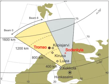
Fig. 1. Field of view of the Hankasalmi HF radar between 400 km and 1600 km and locations of the scintillation receivers (Kokkola, Lulea, Kiruna and Kilpisjarvi) used for tomography derivations of the electron density distribution in the ionosphere.

elevation angles, at least between ∼5◦and ∼50◦(e.g. Arnold et al., 2003). As transmitted radio waves propagate through the ionosphere, they refract and some of them can reach or-thogonality to the magnetic field lines. Such waves have a chance to be backscattered if ionospheric irregularities of proper size exist at ranges of orhtogonality. In this study we postulate that once a radar wave is within ±1◦of off-orthogonality with the Earth magnetic field line, the returned signal is detected. This postulate implies that the ionospheric irregularities exist at all F region heights and that the ir-regularities effectively backscatter the HF radio waves even though they are not exactly elongated with the magnetic field lines. We assume that the irregularities exist anywhere be-tween 150 km and 500 km.

SuperDARN radars record information on the echo range, power, velocity and spectral width (Greenwlad et al., 1995) obtained from the main antennae array. An additional (inter-ferometer) array provides estimates of the elevation angle of echo arrival. In this study, we do not consider the widths and velocity of the echoes with the exception that both parame-ters are used to identify the ionospheric echoes.

In this study, we consider observations by the Hankasalmi HF radar over Northern Scandinavia. Figure 1 shows a part of this radar field-of-view (FoV) between ranges of 400 and 1600 km. In the standard mode of operation, the radar scans through 16 beam positions covering a segment-like area, as shown in Fig. 1. Echoes received in beams 0 to 8 and at ranges 400–1600 km (yellow segment) are considered. This is because the tomographic images of the 2-D electron den-sity distribution in the ionosphere were only available for this part of the Hankasalmi radar FoV. To better explain this point, we show in Fig. 1 by diamonds the locations of

Fig. 2. Hankasalmi echo maps for (a) the power, (b) Doppler ve-locity and (c) elevation angles on 18 May 2003 between 00:10 and 00:12 UT. Frequency of operation was 11.18 MHz.

the scintillation receivers at Kokkola (63.83◦_{N, 23.06}◦_E), Lulea (65.58◦_{N, 22.17}◦_{E), Kiruna (67.84}◦_{N, 20.41}◦_{E) and} Kilpisjarvi (69.02◦_{N, 20.86}◦_{E). One can see that the} to-mography coverage is available for beams 0–8 and for slant ranges from Hankasalmi between ∼400 km and ∼900 km. We add that the tomography measurements are actually avail-able for broader area in terms of latitude because the satel-lites fly roughly along the magnetic meridian and at heights above 500 km so that useful signals for processing begin to be received at elevation angles well off the zenith of each

(4)

station allowing density estimates somewhat equatorward of Kokkola (up to 200 km) and poleward of Kilpisjarvi (up to ranges of ∼1800 km).

It is important to know that Hankasalmi echoes received at ranges of 400–900 km are quite often coming from the E region, sometimes from the F region and sometimes from both the E and F regions (Milan and Lester, 1999). At farther ranges of 900–1500 km, the echoes are usually coming from F region heights. All these types of echoes are expected to be received via the1_/₂_{hop propagation mode, i.e. direct}

ra-dio wave propagation to the scattering area with appropriate amount of refraction. Separation of echo types for each scan is not a simple task; sometimes it can be done by looking at elevation angle information but for many events consid-ered it was not straightforward. In this study, we considconsid-ered only those events for which we were able to separate E and F region scatter confidently. To accomplish this, we first of all were seeking events at ranges >700 km and we used all avail-able information, such as spatial distribution echo parame-ters, elevation angles and distribution of the electron density. Figure 2 gives an example of echoes received by the Han-kasalmi radar on 18 May 2003 between 00:10 and 00:12 UT. Figure 2a shows that the echoes were received from three bands centered at about 800 km, 1300 km and 2200 km. The bands are well defined; the echo bands at far and close ranges are classified as ground scatter by the standard SuperDARN software, Fig. 2b. However, we believe that the short range echoes are actually the ionospheric scatter from the E/upper D regions. Similar observations and interpretation have been presented by Uspensky et al. (2001). Our judgment is also supported by the low values of the elevation angle presented in Fig. 2c. Echoes at the middle ranges are F region1_/

2hop

scatter (these have slightly larger elevation angles than the short range echoes). The present study deals with this type of echo. It is interesting to note that elevation angles for these echoes are largest at the near edge of the echo band and smoothly decrease with range, Fig. 2c, as one would expect if the height of echo is the same at all ranges. Figure 2 also shows a band of ground scatter the farthest ranges. These are beyond the ranges of interest in this study, but we would like to make a note that the elevation angles for some of them are low, in the range of 10◦–15◦, corresponding to the eleva-tion angles of E and F region scatter. This fact indicates that these echoes are received by means of one full hope propa-gation mode via the F region. Some echoes, however, show elevation angles of the order of 25◦_{. These are very likely} obtained through the back (or side) lobe of the Hankasalmi antennae (Milan et al., 1997) though such a judgment is diffi-cult to justify. We will show the ray tracing diagram for this event in Fig. 3 to confirm that reception of echoes at large elevation angles and from forward direction is unlikely.

The example of Fig. 2 gives a sense as to what kind of radar observations were selected for comparison with ray tracing. It was initial intent of this study to use only events with more or less clearly identifiable echo bands so that F

region backscatter at low and high ranges could be resolved confidently. It turned out that finding such events was not an easy task because concurrent data on the electron density distribution of reasonable quality were not so frequent. 2.2 Tomographical determination of the 2-D density

pro-files and event selection

The tomographic method of the 2-D electron density distri-bution determination in the ionosphere has been described by Kunitsyn and Tereshchenko (2003) in general and by Markkanen et al. (1995) and Nygren et al. (1997) with re-spect to the network of scintillation receivers considered in the present study. In short, a chain of several (four in our case) satellite receivers observed signals from Russian Low Earth Orbit satellites. Two signals transmitted coherently at frequencies 150 MHz and 400 MHz were received and their phase difference was used to calculate the ionospheric elec-tron density by means of statistical inversion. A procedure was designed that fits the observed phase values to the startup model of the 2-D electron density distribution. Routine esti-mates were performed by applying two models of the elec-tron density distribution, one was based on a Chapman layer with a peak height at 280 km and another one was based on the IRI model (Bilitza et al., 1997) density distribution over Kokkola shifted down by 50 km. In this study we adopted the IRI-based density distribution estimates; these often show reasonable agreement with concurrent measurements by in-dependent instruments such the EISCAT radar (Nygren et al., 1996). For this choice of startup model, a boundary condition was that the electron density was zero at the ground level. The results of the regularization procedure were presented in terms of the electron density distribution in a vertical plane above the receiver chain. In an ideal case, the satellite would fly in a vertical plane along the chain. For most of passes considered in this study, however, the satellites were off this plane. In these cases, the obtained densities were a projec-tion from regions outside the vertical plane. Because electron density measurements were not obtained exactly along the Hankasalmi meridian, a concern can be raised on the validity of the density distributions. We would like to mention that in this study we consider large-scale characteristics of echo regions and data in multiple radar beams so that the tomog-raphy uncertainties should not obscure the major features of the ionosphere that are important for HF signal.

A sequential search through 2 years of Hankasalmi radar and tomography data, 2003 and 2004, was performed to find appropriate events. It should be remembered that because only 4 receivers were available for the period under study, the electron density distributions were available for limited lat-itude over Northern Scandinavia and limited slant ranges of the Hankasalmi radar, see Fig. 1. In terms of the radar obser-vations, slant ranges between 400 and 1600 km were covered completely by the tomography, and somewhat limited cov-erage was achieved for slant ranges of 1600–1800 km. We

(5)

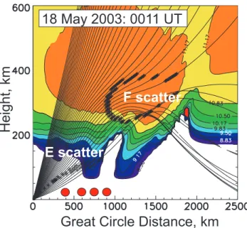
Fig. 3. Electron density distribution along the scintillation re-ceivers meridian and the 2-D ray tracing for the Hankasalmi beam 5 and the event of 18 May 2003, 00:11 UT. Red disks indicate approximate locations of the scintillation re-ceivers. The color coding for the density contours is as fol-lows: blue – between 3.16×108m−3and 6.76×109m−3; green – between 6.76×1010m−3 and 6.76×109m−3; yellow – be-tween 6.76×1010m−3 and 1.48×1011m−3; brown – above 1.48×1011m−3 . Rays are shown in 1◦ step of elevation angle starting from 5◦. The thicker traces correspond to elevation angles of 10◦, 20◦, 30◦and 40◦.

would like to warn the reader that even though the data above 1800 km will be shown, their relevance to the real situation is unknown and we will refrain from comments on radar wave trajectories at ranges >1800 km.

The search for potential events included several steps. First, general quick review of the tomography data on the So-dankyla Geophysical Observatory Web site (http://www.sgo. fi) was performed. Generally, quite a few potentially good events for every day were identified. We sought events with clear and smooth “walls” or boundaries in terms of latitude since, for such events, the correlation with HF echo occur-rence was found to be more obvious. Events at short ranges ∼500–700 km were generally not considered as it was dif-ficult to distinguish E region and F region echo boundaries so that the backscatter height determination was not obvi-ous (see description later). We also avoided observations for which the ionosphere consisted of several density blobs po-tentially leading to a complicated pattern of radar rays in the ionosphere and difficulty in assigning a typical height of an HF echo.

2.3 F region echo height determination

Once joint radar-tomography events were identified, esti-mates of the most likely height of F region echoes were per-formed. To accomplish this task, ray tracing for the Han-kasalmi radar was performed by assuming 2-D electron den-sity distribution (as given by the tomography) for the azimuth of 15◦ west of the geographic meridian which would cor-respond roughly to the Hankaslami beam #6 location. The transmitted frequency in each event was taken into account.

For tracing of the rays we used a program that is based on the Cartesian form of the ray equations developed by Hasel-grove (1963); the Runge-Kutta algorithm for solving the dif-ferential equations was taken from Press et al. (1986). The algorithm uses an adaptive stepsize to reduce the amount of calculations. The program takes into account the wave group delay.

The measured electron density was accepted as a two-dimensional table with values in height and distance from the radar. Interpolation to locations between the table values was done using two-dimensional spline interpolation (also taken from Press et al., 1986), because the tracing program needs both the electron density and its gradient to be without discontinuities. Finally, the IGRF magnetic field model was used for the aspect angle calculations.

Figure 3 illustrates the analysis. In this diagram, the background colored contours describe the electron density distribution in the ionosphere produced by particle precip-itation (the events occurred in the dark ionosphere). Hor-izontally, the great circle distance is used. One can see a large-scale blob of enhanced density between the radar ranges of 200 km and 1800 km. The density inside this blob is above 1.48×1011m−3; the maximum values are of the order 3.2×1011m−3. To check the reliability of the tomographaphic density estimates we considered the ionosonde data collected at Sodankyla (Hankasalmi ranges of ∼650 km). According to Sodankyla ionosonde, the foF2 frequency was 5.1 MHz (at the closest time) which corre-sponds to the density of 3.2×1011m−3_{. Although this value} coincides with the maximum electron density inferred from the tomographic measurements, we should mention that the density maximum according to tomography was achieved at ranges of ∼1000 km from Hankasalmi. At ranges of Sodankyla ionosonde location (∼650 km), the density was somewhat smaller, 2.5×1011m−3. We attribute this rather small difference to the longitudinal separation for the areas of the tomographic and ionosonde measurements and some errors in tomography analysis.

In Fig. 3, electron density decreases strongly toward lower heights so that at ∼200 km it is of the order of 1010m−3; such densities do not affect the Hankasalmi radio wave paths significantly. Figure 3 also shows paths of various rays in the ionosphere taking off at elevation angles ε of 5–45◦. The traces for ε=10◦, 20◦, 30◦, and 40◦are shown by thicker line to facilitate the diagram overview. Each cross along a ray

(6)

trace indicates that part of the ray trajectory where the ray is within ±1◦_{of the off-orgothonality condition thus signifying} a possibility of echo detection at this specific range. One can notice a cloud of crosses at ranges of 200–800 km and heights of 50–120 km and a horse-shoe like cloud of crosses at ranges 900–1800 km and heights of 230–350 km. These two clouds are the expected locations, in range and height, of E region echoes (between 90 and 120 km) and F region echoes.

Figure 3 shows that F region echoes can come from quite a range of heights and great circle distances. An important feature of the prediction is that echoes are expected at all ranges from 900 km up to 1800 km, in terms of the great circle distance. These numbers should be increased by 50– 150 km, if the distances are counted in terms of the radar slant range. Actual radar data show that the echoes cover the band of 1035–1755 km, Fig. 2, for the scan under consideration. The range extension of the band is 720 km and the band’s short range border is shifted poleward by ∼85 km from what is predicted. We attribute this shift to a slight error in to-mographic electron density estimates and decide that only ranges from 950 to 950+720=1670 km have to be considered in model estimates of the scatter height. The predicted poten-tial scatter from farther ranges of 1670 km (once again, used in Fig. 3 great circle ranges are shorter than slant ranges of echoes, see also later Fig. 4) is not counted as the observa-tion does not show such echoes. Similar consideraobserva-tion and judgment were applied for each individual event; the differ-ences between the model predictions and measurements at the shortest ranges of an echo band of up to 100 km were al-lowed. We admit that the procedure of echo ranges cutoff is somewhat subjective.

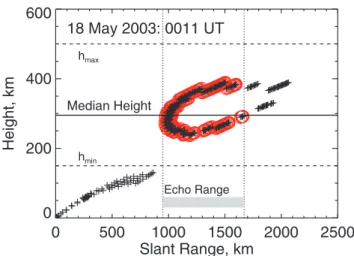
Figure 4 explains how the “typical” height was determined for each individual event. Here we show the slant ranges, the actual ranges along curved trajectories (Fig. 3 uses great circle distance which can be up to ∼100 km shorter) and the heights of expected orthogonal intersections according to ray tracing of Fig. 3. We also show by red circle every point which is within the band of possible slant ranges of echoes according to radar measurements. There are 183 such points. The median value for the height of all these points (horizontal line in Fig. 4) was considered to be the most likely height of F region echoes. For this specific event, this value turned out to be 297 km. We also computed the average height for crosses with red circles in Fig. 4; the average height was found to be 306 km. This is a very typical situation that the mean and median values do not differ much.

We should mention that the median value was counted for all crosses located between heights of hmin=150 km and

hmax=500 km, the assumed height range of the irregularity

layer. For the event under consideration, the orthogonality condition was met in rather limited band of heights. To char-acterize the height extent of echo region, we computed the difference between the lowest and highest points for each di-agram; for the 18 May 2003 event, it was ∼149 km. We call this parameter the thickness of the backscatter layer.

Fig. 4. Diagram illustrating the method of echo height estimation for the event of 18 May 2003, 00:11 UT.

One can also notice that, according to Figs. 3 and 4, at some ranges the echoes are expected to come from two iono-spheric heights with significantly different elevation angles. This expected feature of HF echo detection was discussed by Andre et al. (1997) and earlier by Uspensky et al. (1994) with respect to the E region observations. We note that expected elevation angles for the top and bottom parts of the scattering layer are largest at shorter ranges and decrease with range, Fig. 3. The effect is more pronounced for the echoes com-ing from the bottom part of the scattercom-ing layer. Actual radar data of Fig. 2 do show the elevation angle decrease clearly, as mentioned earlier, but whether the scatter is coming from two heights is difficult to judge from the data available. The fact that the elevation angles fall very quickly with range in Fig. 2 gives a hint that perhaps the top part of the expected scattering layer is less effective. This implies that the height estimates presented below are perhaps the upper limit of pos-sible heights.

2.4 Statistical results

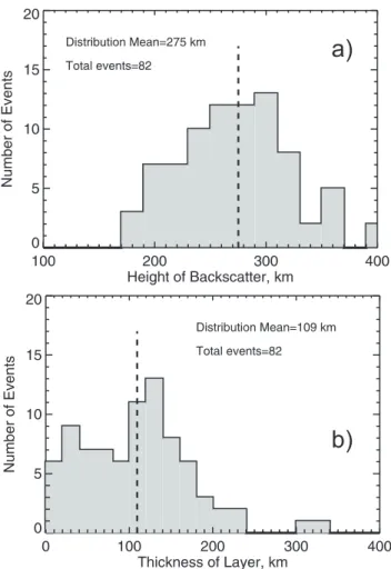
A systematic search through joint radar-tomography data base allowed us to identify 82 events for which determina-tion of the most likely F region echo height was possible. Figure 5 summarizes our findings for (a) the height and (b) the thickness of the backscatter layer. The distribution for the echo height in Fig. 5a has a bell-like shape, slightly skewed toward smaller heights. The distribution peaks at ∼280 km, and the average height is 275 km. In individual cases, the height can be below 200 km and above 350 km. Distribution for the backscatter thickness is more uniform; there is about equal possibility of thickness between 10 and 150 km with somewhat preferential values of 120–130 km.

(7)

Fig. 5. Histogram distributions for (a) the heights of1_/₂_hop

prop-agation F-region echoes and (b) the altitudinal spread of expected echo heights (thickness of backscatter layer) for the entire data set of 82 events.

3 Discussion and summary

Measurements of the height of SuperDARN HF echoes is a challenging problem, and so far not much has been estab-lished. Previous ray tracings showed that HF radars are very sensitive to the electron density distribution in the ionosphere so that perpendicularity with the magnetic field lines can be achieved over a broad range of heights (Villain et al., 1984; Andre et al., 1997; Danskin, 2003). Villain et al. (1984) ex-pected typical heights of more than 300 km while Danskin et al. (2002) and Danskin (2003) predicted rather low heights of <250 km. These previous studies suggest that the1_/

2hop

F region scatter is typically coming from heights below the F region density peak. Milan and Lester (2001) presented estimates of the apparent F region echo heights using Han-kasalmi interferometer data. Their Fig. 1 shows preferential heights of 220–230 km. The real heights in this experiment should be even smaller, implying fairly low F region echo heights. It is important to realize that these observations were performed, most likely, at short ranges as the

experi-Fig. 6. Heights of the orthogonality condition (with refraction taken into account) for the Hankasalmi radar at ranges 500, 800, 1000, 1200 and 1500 km. A uniform electron density distribution, both horizontally and vertically, is assumed.

ment was run in the so called “myopic mode” with range bins of 15 km instead of standard 45-km bins. All the above pre-dictions and measurements indicate great variability in the height of F region backscatter at HF; this is very likely be-cause of the highly variable electron density distribution in the auroral zone (especially during frequent particle precipi-tation events) and also because the irregularities might exist in certain layers rather than throughout the entire F region.

Milan et al. (1999) established and later Danskin et al. (2002) confirmed that Hankasalmi1_/₂_{hop F region echoes}

near EISCAT (ranges ∼900 km) occur preferentially for the electron density of ∼2×1011m−3_{. Simple ray tracing for} vertically stratified (i.e. horizontally uniform) ionosphere for the Hankasalmi radar geometry shows that for such electron densities, the scatter should be coming from ∼250 km. To illustrate this point, we show in Fig. 6 the required densi-ties at various heights so that the radar wave reaches or-thogonality. Five ranges from Hankasalmi are considered. One can see, quite generally, that for electron densities be-low 1.5×1011m−3the echoes are expected to come mostly from the heights <250 km over a broad band of ranges 800– 1500 km, including the range of EISCAT location. These are exactly the ranges of echoes that we considered in this study. With the electron density increase, echoes can be de-tected at shorter ranges and at heights below 200 km. Our re-examination of the data used in Fig. 5 showed that indeed for all reported low-height events of <210 km, the minimum echo ranges were below 900 km. This result implies that if one selects only short range Hankasalmi events, the his-togram of Fig. 5 would maximize at much lower heights. We also should mention that in a case of two-layer scattering, as in the example of Fig. 3, the upper layer might not always be effective, as discussed earlier, implying that the estimated typical heights can be smaller. In this study, the events were

(8)

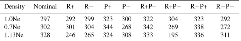
Table 1. Expected median heights of Hankasalmi echoes for a number of electron density distributions that are modifications of the one shown in Fig. 3. Density Nominal R+ R− P+ P− R+P+ R+P− R−P+ R−P− 1.0Ne 297 292 299 323 300 322 304 323 292 0.7Ne 302 301 304 344 268 342 269 338 272 1.13Ne 328 246 265 324 308 333 195 336 311

selected randomly, and we think that Fig. 5 gives at least a good first estimate of what are the typical heights of the Han-ksalmi F region echoes at ranges 700–1500 km. The inferred “typical height” of F region echoes of 275 km supports the choice of 300 km for the height of echoes adopted in the Su-perDARN processing software, including the Map Potential technique of Ruohoniemi and Baker (1998).

The Hankasalmi1_/₂_{-hop F region echo heights estimates}

reported in this study depend strongly on the quality of the electron density distributions provided by the tomographic measurements. Unfortunately, reliability of the tomographic inversion technique that was employed in this study is not well established. Nygren et al. (1996) presented data validat-ing the method for a subset of data, but reliability of density distributions for any time remains unclear. For one thing, the density distributions obtained by employing different startup density distributions with height are somewhat different in magnitude as one can witness by viewing data on the So-dankyla website. We hope that additional criterion for data selection allowed us to select periods with reasonable tomo-graphic estimates; namely, we selected only those events for which the expected ranges of HF echoes were about the same as the ranges of observed echoes. To evaluate impact of un-certainty in the electron density distribution measurements on obtained results we performed a series of ray tracings with electron density distributions that were modifications of the one presented in Fig. 3. We used this profile but shifted it away (R+) or towards (R−) the radar location by 111 km (one degree of latitude) or shifted it up (P+) or down (P−) by 30 km. Combinations of the range and height shifts were also considered. We then repeated ray tracings by assum-ing that the densities are increased (decreased) by a factor of 1.3 (0.7). Results of this analysis for the median height are presented in Table 1.

First raw in Table 1 shows that shifting of the density dis-tribution of Fig. 3 in range (by +/−111 km) or height (by +/−30 km) does not give significant change in the echo me-dian height. It is 5–20 km from the nominal height of 297 km. Similar conclusion can be made for the density distribu-tions with the reduced magnitude, second raw, except max-imum difference from the nominal height can be as large as ∼45 km, both ways, positive and negative. For the case of in-creased densities (by 1.3 times, third raw in Table 1), change in the expected echo height is more prominent, up to 100 km, with the strongest change occurring for the profile shifted

away (change is 297–246=51 km) and away and down si-multaneously (change is 297–195=102 km). The performed estimates indicate that if the electron densities were some-what larger than the ones used in this study, then the overall expected height of Hankasalmi echoes of 275 km would be somewhat smaller, perhaps by ∼10–30 km.

This paper considered echo heights only in terms of prop-agation conditions. Milan et al. (1998) showed that statis-tically, irrespective of propagation conditions, dayside HF echoes occur preferentially within the auroral oval (where electric fields and plasma density gradients are both en-hanced) implying that irregularity production is very impor-tant factor for echo detection. We considered only those events for which echoes were seen, and we were sure that irregularities did exist in the ionosphere. Less certain was the assumption that decameter irregularities existed at all F region heights where orthogonality condition was met. If this was not the case, our estimates of typical height might be erroneous. Unfortunately, not much is known in terms of the irregularity production heights. If one assumes that the gradient-drift instability (e.g. Tsunoda, 1988) is the main source of decameter F region irregularities, then one may ex-pect irregularity production at just about any height as the in-stability conditions do not change much with the height. Ba-sically, having enhanced electric field and steep enough elec-tron density gradient are enough to set the instability going. Certainly, the key question is whether gradients are present at all heights and at any instant of time. In addition, the role of the other factors, such as presence of highly conducting E region, need to be evaluated. Joint radar-tomographic obser-vations complemented with scintillation detection of F region irregularities could be useful for future studies.

Results of this study can be summarized as follows. 1. Ray tracing analysis based on tomographic estimates of

the 2-D electron density distribution within the field of view of the Hankasalmi HF radar showed that the most likely height of the F region echoes received through

1_/₂ _{hop propagation mode at ranges 700–1500 km is}

∼275 km. The typical thickness of the backscatter layer, inferred from the analysis of propagation conditions only, is of the order of 100 km.

2. In individual events, echo heights of more than 350 km and less than 200 km are possible.

(9)

1994 A. V. Koustov et al.: Heights of SuperDARN F region echoes 3. Cases of Hankasalmi radar F region echo detection at

very short ranges of <700 km when the echoes are very likely to be a mixture of scatter from the bottom-side F region and the electrojet E region were not considered and require further investigation.

Acknowledgements. We thank the U of Leicester radar group (M. Lester, PI) that continuously operated the Hankasalmi HF radar and provided data used in this study. Help of L. V. Benkevitch in data processing is appreciated. This work has been supported by NSERC (Canada) grant to A. V. Koustov.

Topical Editor M. Pinnock thanks M. Uspensky and P. L. Dyson for their help in evaluating this paper.

References

Andre, R., Hanuise, C., Villain, J.-P., and Cerisier, J.-C.: HF radars: Multifrequency study of refraction effects and localization of scattering, Radio Sci., 32, 153–168, 1997.

Arnold, N. F., Cook, P. A., Robinson, T. R., Lester, M., Chapman, P. J., and Mitchell, N.: Comparison of D-region Doppler drift winds measured by the SuperDARN Finland HF radar over an annual cycle using the Kiruna VHF meteor radar, Ann. Geophys., 21, 2073–2082, 2003,

http://www.ann-geophys.net/21/2073/2003/.

Bilitza, D.: International Reference Ionosphere: Status 1995/96, Adv. Space Res., 20(9), 1751–1754, 1997.

Bristow, W. A., Sofko, G. J., Stenbaek-Nielsen, H. C., Wei, S., Lummerzheim, D., and Otto, A.: Detailed analysis of sub-storm observations using SuperDARN, UVI, ground-based mag-netometers, and all-sky imagers, J. Geophys. Res, 108(A3), 1124, doi:10.1029/2002JA009242, 2003

Danskin, D. W., Koustov, A. V., Ogawa, T., Nishitani, N., Nozawa, S., Milan, S. E., Lester, M., and Andr´e, D.: On the factors con-trolling occurrence of F-region coherent echoes, Ann. Geophys., 20, 1385–1397, 2002,

Danskin, D. W.: HF auroral backscatter from the E and F regions, PhD thesis, U of Saskatchewan, Saskatoon, SK, Canada, 2003. Greenwald, R. A., Baker, K. B., Dudeney, J. R., Pinnock, M., Jones,

T. B., Thomas, E. C., Villain, J.-P., Cerisier, J.-C., Senior, C., Hanuise, C., Hunsuker, R. D., Sofko, G., Koehler, J., Nielsen, E., Pellinen, R., Walker, A. D. M., Sato, N., and Yamagishi, H.: DARN/SuperDARN: A global view of the dynamics of high-latitude convection, Space Sci. Rev., 71, 763–796, 1995. Haselgrove, J.: The Hamiltonian ray path equations, J. Atmos. Terr.

Phys., 25, 397–399, 1963.

Kozlovsky, A., Koustov, A., Lyatsky, W., Kangas, J., Parks, G., and Chua, D.: Ionospheric convection in the postnoon auroral oval: Super Dual Auroral Radar Network (SuperDARN) and Polar ul-traviolet imager (UVI) observations, J. Geophys. Res., 107(12), 1433, doi:10.1029/2002JA009261, 2002.

Kunitsyn, V. E. and Tereshchenko, E. D.: Ionospheric tomography, Springer-Verlag, Berlin, 2003.

Lyons, L. R., Liu, S., Ruohoniemi, J. M., Solovyev, S. I., and Samson, J. C.: Observations of dayside convection reduction leading to substorm onset, J. Geophys. Res., 108(3), 1119, doi:10.1029/2002JA009670, 2003.

Markkannen, M., Lehtinen, M., Nygren, T., Pirttila, J., Heneli-uus, P., Vilenius E., Tereshchenko, E. D., and Khudukon, B.

Z.: Bayesian approach to satellite radiotomography with applica-tions in the Scandinavian sector, Ann. Geophys., 13, 1277–1287, 1997,

Milan, S. E., Jones, T. B., Robinson, T. R., Thomas, E. C., and Yeoman, T. K.: Interferometric evidence for the observation of ground backscatter originating behind the CUTLASS coherent HF radars, Ann. Geophys., 15, 29–39, 1997,

Milan, S. E., T. K. Yeoman, T. K., and Lester, M.: The dayside auroral zone as a hard target for coherent HF radars, Geophys. Res. Lett., 25, 3717–3720, 1998.

Milan, S. E., Davies, J. A., and Lester, M.: Coherent HF radar backscatter characteristics associated with auroral forms identi-fied by incoherent radar techniques: A comparison of CUTLASS and EISCAT observations, J. Geophys. Res., 104, 22 591–22 604, 1999.

Milan, S. E. and Lester, M.: A classification of spectral populations observed in HF radar backscatter from the E region auroral elec-trojets, Ann. Geophys., 19, 189–204, 2001,

Nygren, T., Markkanen, M., Lehtinen, M., Tereshchenko, E. D., Khudukon, B. Z., Evstafiev, O. V., and Pollari, P.: Comparison of F-region electron density observations by satellite radio to-mography and incoherent scatter methods, Ann. Geophys., 14, 1422–1428, 1996,

Nygren, T., Markkanen, M., Lehtinen, M., Tereshchenko, E. D., and Khudukon, B. Z.: Stochastic inversion in ionospheric radioto-mography, Radio Sci., 32, 2359–2372, 1997.

Oksavik, K., Ruohoniemi, J. M., Greenwald, R. A., Baker, J. B. H., Moen, J., Carlson, H. C., Yeoman, T. K., and Lester, M.: Obser-vations of isolated polar cap patches by the European Incoher-ent Scatter (EISCAT) Svalbard and Super Dual Auroral Radar Network (SuperDARN) Finland radars, J. Geophys. Res., 111, A05310, doi:10.1029/2005JA011400, 2006.

Press, W., Flannery, B., Teukolsky, S., and Vetterling, W.: Numeri-cal recipes, the art of scientific computing, Cambridge University Press, 1986.

Ruohoniemi, J. M. and Baker, K. B.: Large-scale imaging of high-latitude convection with Super Dual Auroral Radar Network HF radar observations, J. Geophys. Res., 103, 20 797–20 811, 1998. Tsunoda, R. T.: High latitude irregularities: A review and synthesis,

Rev. Geophys., 26, 719–760, 1988.

Uspensky, M., Eglitis, P., Opgenoorth, H., Starkov, G., Pulkkinen, T. and Pellinen, R.: On auroral dynamics observed by HF radar: 1. Equatorward edge of the afternoon-evening diffuse luminosity belt, Ann. Geophys., 18, 1560–1575, 2001,

Uspensky, M. V., Kustov, A. V., Sofko, G. J., Koehler, J. A., Villain, J.-P., Hanuise, C., Ruohoniemi, J. M., and Williams, P. J. S.: Ionospheric refraction effects in slant range profiles of auroral HF coherent echoes, Radio Sci., 29, 503–517, 1994.

Villain, J. P., Greenwald, R. A., and Vickery, J. F.: HF ray trac-ing at high-latitudes ustrac-ing measured meridional electron density distributions, Radio Sci., 19, 359–374, 1984.

Yeoman, T. K., Wright, D. M., Stocker, A. J., and Jones, T. B.: An evaluation of range accuracy in the SuperDARN over-the-horizon HF radar systems, Radio Sci., 36, 801–813, 2001.