The impact of PMSE and NLC particles on VLF propagation

(1)

HAL Id: hal-00317333

https://hal.archives-ouvertes.fr/hal-00317333

Submitted on 8 Apr 2004

HAL is a multi-disciplinary open access

archive for the deposit and dissemination of

sci-entific research documents, whether they are

pub-lished or not. The documents may come from

teaching and research institutions in France or

abroad, or from public or private research centers.

L’archive ouverte pluridisciplinaire HAL, est

destinée au dépôt et à la diffusion de documents

scientifiques de niveau recherche, publiés ou non,

émanant des établissements d’enseignement et de

recherche français ou étrangers, des laboratoires

publics ou privés.

propagation

D. Nunn, M. A. Clilverd, C. J. Rodger, N. R. Thomson

To cite this version:

D. Nunn, M. A. Clilverd, C. J. Rodger, N. R. Thomson. The impact of PMSE and NLC particles on

VLF propagation. Annales Geophysicae, European Geosciences Union, 2004, 22 (5), pp.1563-1574.

�hal-00317333�

(2)

SRef-ID: 1432-0576/ag/2004-22-1563 © European Geosciences Union 2004

Annales

Geophysicae

The impact of PMSE and NLC particles on VLF propagation

D. Nunn1, M. A. Clilverd2, C. J. Rodger3, and N. R. Thomson3

1_{Dept. of Electronics and Computer Science, Southampton University, Southampton SO17 1BJ, UK} 2_{British Antarctic Survey, Cambridge, CB3 0ET, UK}

3_{Dept. of Physics, University of Otago, Dunedin, New Zealand}

Received: 4 August 2003 – Revised: 6 January 2004 – Accepted: 14 January 2004 – Published: 8 April 2004

Abstract. PMSE or Polar Mesosphere Summer Echoes are

a well-known phenomenon in the summer northern polar gions, in which anomalous VHF/UHF radar echoes are re-turned from heights ∼85 km. Noctilucent clouds and elec-tron density biteouts are two phenomena that sometimes oc-cur together with PMSE. Electron density biteouts are elec-tron density depletion layers of up to 90%, which may be several kms thick. Using the NOSC Modefndr code based on Wait’s modal theory for subionospheric propagation, we calculate the shifts in received VLF amplitude and phase that occur as a result of electron density biteouts. The code as-sumes a homogeneous background ionosphere and a homo-geneous biteout layer along the Great Circle Path (GCP) cor-ridor, for transmitter receiver path lengths in the range of 500–6000 km.

For profiles during the 10 h about midnight and under quiet geomagnetic conditions, where the electron density at 85 km would normally be less than 500 el/cc, it was found that re-ceived signal perturbations were significant, of the order of 1–4 dB and 5–40◦of phase. Perturbation amplitudes increase roughly as the square root of frequency. At short range perturbations are rather erratic, but more consistent at large ranges, readily interpretable in terms of the shifts in excita-tion factor, attenuaexcita-tion factor and v/c ratios for Wait’s modes. Under these conditions such shifts should be detectable by a well constituted experiment involving multiple paths and multiple frequencies in the north polar region in summer. It is anticipated that VLF propagation could be a valuable di-agnostic for biteout/PMSE when electron density at 85 km is under 500 el/cc, under which circumstances PMSE are not directly detectable by VHF/UHF radars.

Key words. Electromagnetism (wave propagation) –

Iono-sphere (polar ionoIono-sphere) – Radioscience (ionospheric prop-agation)

Correspondence to: D. Nunn

(dn@ecs.soton.ac.uk)

1 Introduction

Polar Mesospheric Summer Echoes (PMSE) have been ob-served at VHF and UHF frequencies (Cho and Rottger, 1997) as strong radar echoes from near the altitude of the Northern Hemisphere polar summer mesopause, located at ∼85 km al-titude. It has been suggested that there is a possibility of ob-serving the echoes at MF (Murphy and Vincent, 2000). All of these techniques involve the analysis of the return echo from radio waves launched in a near vertical direction by high power antenna arrays (Bremer et al., 1995). Observa-tions have been mainly confined to the North Polar regions, though PMSE have been reported in Antarctica and also at mid-latitudes. PMSE events can last for more than an hour in some cases, often being seen for more than 30 min at a time (Palmer et al., 1996). The reflecting layers which lead to PMSE may have multiple structures and move dynamically on a time scale of minutes (Bremer et al., 1996). Theoretical investigations of the causes of PMSE are still ongoing, and are undoubtedly very complex. The phenomenon is clearly related to the extreme low temperatures prevailing at the summer mesopause, primarily in polar regions. PMSE are believed to result from scattering by enhanced small-scale spatial electron density fluctuations, arising from diminished electron density diffusivities due to the action of sub-visible aerosols, probably ice. From both observational and theoret-ical evidence, a minimum electron density exists at ∼85 km altitude of approximately 500 el/cc that is required to produce observable VHF/UHF radar echoes (Rapp et al., 2002). Be-low this density threshold the scattering of VHF/UHF waves becomes too weak to produce a detectable echo. It should be noted that interest in PMSE is not entirely confined to iono-spheric plasma physicists. Since PMSE and related phenom-ena are critically dependent on the extremely low tempera-tures prevailing at the polar summer mesopause, the occur-rence of PMSE may be a critical indicator of climate change and global warming (Bremer et al., 2003)

(3)

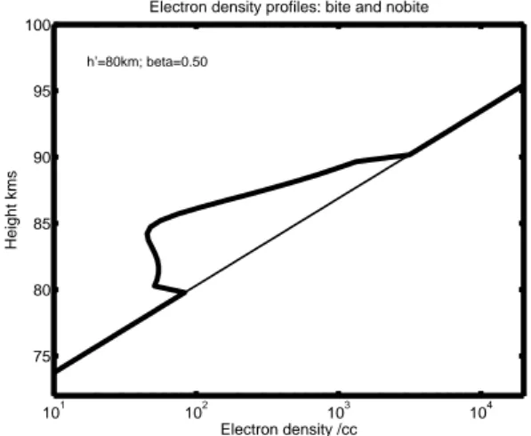
101 102 103 104 75 80 85 90 95 100

Electron density profiles: bite and nobite

Electron density /cc

Height kms

h’=80km; beta=0.50

Fig. 1. Plot of ambient electron density profile and perturbed profile showing biteout.

Electron density “biteouts” have on occasion been ob-served by rocket instruments while radars have obob-served PMSE at adjacent heights (e.g. Ulwick et al., 1988), but PMSE do often occur without nearby electron density “bite-outs” (Hoppe et al., 1994; Blix et al., 2003). Recent rocket campaigns at high latitudes have provided a significant num-ber of D-region electron concentration profiles at the time of occurrence of PMSE (Goldberg et al., 2001). Typically “biteouts” in electron concentration occur near the altitudes of noctilucent clouds (Ulwick et al., 1988; Blix et al., 2003) and are thought to be due to the presence of aerosols scaveng-ing lower ionospheric free electrons (Croskey et al., 2001). The “biteouts” are typically found at about 85 km, have an altitude span of several kms, and have electron concentration levels that are reduced by around ten times.

Experimental observations of PMSE and electron density biteouts are confined to specific geographic locations and very limited information exists as to the spatial distribution of these phenomena at a specific time. Bremer et al. (1996) showed that significant similarities in PMSE observations could be detected over distances of 130 km, although local features can be modified by processes such as gravity waves (Bremer et al., 1995). Radar cross section observations can change dramatically within a few minutes, which is also an indication of horizontal patchiness.

PMSE are sometimes observed in association with noc-tilucent clouds (NLC) (Thomas, 1991; Pfaff et al., 2001), although not always (Taylor et al., 1989). A mechanism to explain these observations has been suggested through sub-visible electron-scavenging particles (which produce elec-tron density biteouts) evolving to larger dimensions, sedi-menting to lower altitude, and becoming visible optically as NLC (Hoppe et al., 1994). The two phenomena are simi-larly associated with the very cold summer polar mesosphere (Palmer et al., 1996). NLC occurs at ∼82 km in height, just below the altitude associated with PMSE, and consist of vis-ible ice aerosols. Typically NLC are large-scale features, of-ten being observed above significant fractions of the polar

re-gions. Similar large-scale biteout structures could influence the propagation of long-path radio waves that reflect from the lower ionosphere near 85 km altitudes.

Here we use the well-developed NOSC long wave prop-agation model to investigate the impact of large-scale “bite-outs” on the signal from very low frequency (VLF) trans-mitters over a range of frequencies (20–80 kHz) and for transmitter-receiver path lengths varying from 500–6000 km. Radio waves from manmade VLF transmitters propagate in-side the waveguide formed by the lower ionosphere and the Earth’s surface. Significant variations in the received ampli-tude and phase arise from changes in the lower ionosphere. These variations include those driven by changes in solar zenith angle (Thomson, 1993), solar flares (Deshpande and Mitra, 1972), lightning-induced electron precipitation (Hel-liwell et al., 1973), and red sprites (Hardman et al., 1998). Further discussion on the use of subionospheric VLF propa-gation as a remote sensing probe can be found in recent re-view articles (e.g. Barr et al., 2000; Rodger, 2003). We will show that significant phase and amplitude changes in VLF propagation may be observed when large-scale biteouts are present, and that it should be possible to detect such changes when ambient electron density concentration levels at 85 km are below ∼500 el/cc, under which circumstances PMSE it-self is not directly detectable by radar. The probing of elec-tron density biteouts through subionospheric VLF propaga-tion would provide a complementary observapropaga-tion technique and provide additional information about the scale and nature of electron biteouts and, by association, PMSE and NLC.

2 The influence of biteouts on subionospheric VLF

propagation

VLF wave propagation codes, such as MODEFNDR and LWPC (Ferguson and Snyder, 1990), utilising Wait’s clas-sic modal theory (Wait and Spies, 1964; Wait, 1996), can be used to model the propagation of waves within the Earth-ionosphere waveguide and can therefore be used to investi-gate the impact of the electron concentration “biteouts”. Al-though the vertical extent of the “biteouts” is typically less than the wavelength at VLF (about 10 km), the oblique na-ture of the reflection at the upper boundary of the waveguide suggests that some changes in the VLF propagation charac-teristics of narrow-band signals from terrestrial VLF trans-mitters might be anticipated.

At mid-latitudes the background electron density profile at D-region altitudes is reasonably defined within VLF prop-agation codes by using the following equation for the elec-tron density profile Ne(z)(in electrons per cubic centimetre)

(Wait and Spies, 1964),

Ne(z) =7.855 × 10−5eβ(z−h 0₎

ν(z), (1)

where collision frequency ν (in collisions per second) is given by

(4)

0 5 10 15 0.5 1 1.5 2 2.5 v/c dominant modes;F=20kHz Mode number v/c TM Modes TE Modes 0 5 10 15 10−1 100 101 102 Attenuation factor Mode number Attenuation dB/Mm TM Modes TE Modes 0 5 10 15 0 0.5 1 1.5

Excitation factor |lamda|

Mode number

Abs. excitation factor TM Modes

TE Modes 0 5 10 −80 −60 −40 −20 0

Mode amplitude/ range=500,6000km

Mode number

Mode significance dB

500km

6000km

TM Modes TE Modes

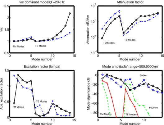
Fig. 2. Modal parameters at f =20 kHz for the profile given by h0=80 km, β=0.5 km−1. The solid lines are for the unperturbed profile, the

dashed blue lines for the profile with biteout. The fourth panel shows modal amplitudes at the receiver at a range of 500 km, the black line with circles being with no biteout, the blue line with circles with biteout. The corresponding figures at a range 6000 km are given by the dashed green line with crosses (biteout) and red line with crosses (no biteout).

0 5 10 15

−1 −0.5 0 0.5

v/c shift due to biteout;F=20kHz

Mode number v/c TM Modes _{TE Modes} 0 5 10 15 −20 −10 0 10 20 30

Attenuation factor shift

Mode number Attenuation dB/Mm TM Modes TE Modes 0 5 10 15 −0.5 0 0.5 1

Excitation factor shift

Mode number

TM Modes TE Modes 0 5 10 15 −200 −150 −100 −50 0 50 100

Mode amplitude shift/range=500,6000km

Mode number

500km 6000km

TM Modes TE Modes

Fig. 3. Perturbations of modal parameters at f =20 kHz due to the biteout. The fourth panel shows change in modal composition, where the black line with circles is for a range of 500 km and the green line with crosses is for 6000 km. Important features are the increased attenuation and increased phase velocity of dominant TM modes.

(5)

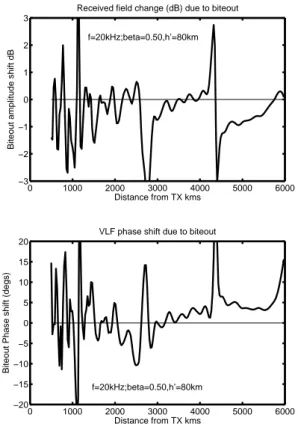
0 1000 2000 3000 4000 5000 6000 −3 −2 −1 0 1 2 3

Received field change (dB) due to biteout

Distance from TX kms

Biteout amplitude shift dB

f=20kHz;beta=0.50,h’=80km 0 1000 2000 3000 4000 5000 6000 −20 −15 −10 −5 0 5 10 15 20

VLF phase shift due to biteout

Biteout Phase shift (degs)

f=20kHz;beta=0.50,h’=80km

Fig. 4. Change in received amplitude and phase of subionospheric VLF propagation, due to biteout. The graph is for f =20 kHz and is plotted as a function of range. The perturbation is generally negative

(typically ∼−1 dB) and positive phase (typically ∼4◦) with spikes

at modal interference minima. Propagation at short range is strongly multimodal, and received amplitude is rather unpredictable.

and z is the altitude in kilometres. Here, β represents the “sharpness” of the lower ionospheric boundary and h0 rep-resents the effective height of the ionosphere. Friedrich and Kirkwood (1999) show that at higher latitudes of 60–70◦this parameterisation can still hold during quiet geomagnetic con-ditions. Inspection of published rocket profiles shows that at the time and place of PMSE events under well illumi-nated conditions, the electron density profiles have values of ∼4000 el/cc at 85 km altitude, which is consistent with the typical value reported by Rapp et al. (2002). Typical “night-time” values for β and h0_{at high latitudes during the}

summer months are likely to be 0.30 km−1 _{and 76 km,}

re-spectively, which give 500 el/cc at 85 km altitude (Thomson, 1993; McRae and Thomson, 2000; Friedrich et al., 2002). This coincides with the minimum 85 km background elec-tron concentration for PMSE VHF/UHF radar observations. However, as shown below, VLF propagation characteristics should be even more sensitive to “biteouts” during periods of lower electron density background levels, although these would be unlikely to occur for much of the time during well-illuminated polar summer conditions.

2.1 Details of the computation of VLF propagation pertur-bations

Our code calls as a subroutine a computer program developed by NOSC (Naval Ocean Systems Center, San Diego, USA) which returns all the parameters of the subionospheric VLF modes as described by Wait (1996). This program receives as inputs the frequency, ionospheric and geomagnetic param-eters. Then, assuming horizontal homogeneity, the program calculates the appropriate full wave reflection coefficients for the waveguide boundaries and searches for those modal an-gles which give a phase change of 2π across the guide. The computations take into account the curvature of the Earth, not by means of a spherical coordinate system, but by adding a radially dependent corrective term to the refractive index. A version of the program called MODESRCH is described and listed (in FORTRAN) by Morfitt and Shellman (1976). The program used for the mode parameter calculations reported here is a slightly modified version of the NOSC program MODEFNDR which is very similar to MODESRCH. Fur-ther discussion of the very complex mathematical details of the NOSC VLF propagation program and comparisons with experimental data can be found in Bickel et al. (1970) and Pappert and Hitney (1988).

The output of MODEFNDR then comprises the excitation factors, height gain functions, attenuation factors and hori-zontal wave numbers for allowable VLF modes. The main code uses modal theory to compute the amplitude and phase of the received VLF signal at zero altitude as a function of range from the transmitter. The field component computed is the vertical electric field Ez. In order to match the

config-uration of high power USN VLF transmitters, such as NAA (44◦38’ N, 067◦17’ W, ∼1 MW), the transmitter is also as-sumed to be at zero altitude and comprises a vertical electric dipole. It should be pointed out that a transmitter built for re-search purposes, such as the Siple VLF station in Antarctica (Helliwell, 1988), could well adopt the alternative configu-ration of a horizontal electric dipole overlaying a low con-ductivity medium, such as ice or rock. In this case the prop-agation calculations would need to be redone. The selected frequencies are 20, 40, 60, and 80 kHz. The first of these corresponds closely to the frequencies used by USN VLF transmitters. The higher frequencies are intended to explore the frequency dependence of the biteout effect and also to inform experimental choices where various transmitters are available for use or may be specially constructed for research purposes.

The code uses all the modes returned by MODEFNDR, both TE and TM, in the modesum operation. The total num-ber of modes used varies from 21 to about 60, depending on the transmitter frequency.

The path length between the transmitter and receiver is taken to vary from 500 km to 6000 km and to be over sea. Wait’s modal theory will hold throughout our range of path lengths. The long path we have chosen might correspond to a transpolar path at about 60◦latitude. For most of the calcu-lations we have used an undisturbed ionospheric profile with

(6)

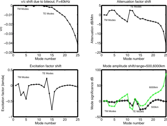
0 5 10 15 20 25 −0.05 −0.04 −0.03 −0.02 −0.01 0

v/c shift due to biteout; F=40kHz

Mode number v/c TM Modes TE Modes 0 5 10 15 20 25 −20 −15 −10 −5 0 5

Mode number Attenuation dB/Mm TM Modes TE Modes 0 5 10 15 20 25 −1 −0.5 0 0.5

Mode number

TM Modes TE Modes 0 5 10 15 20 25 −50 0 50 100

Mode number

Mode significance dB 500km

6000km

TM Modes TE Modes

Fig. 5. Shifts in modal parameters at f =40 kHz. Dominant modes are TM2–TM4. TE15 is of significance at short range and TE12–13 at longer ranges. Important features are increased attenuation and lower excitation for dominant modes TM3–TM5 and TE12.

β=0.50 and h0=80 km, which gives an ambient electron den-sity at 85 km of 500 el/cc and corresponds to a “night-time” low illumination situation. This electron density lies at the lower limit of PMSE detection in radar data, and is at the upper limit of biteout detection from VLF, as will be shown below. The background ionosphere is assumed to be homo-geneous along the entire GC path, which will not be true for long paths. The code LWPC has the capability of dealing with long inhomogeneous paths and can calculate continu-ously the inter modal conversion that takes place along the GC path due to the inhomogeneity. However, LWPC is not an easy tool to use for scientific research. MODEFNDR re-quires a number of parameters, which are taken to be those appropriate to 68◦geographic latitude, namely ambient mag-netic field strength (B=5.3×10−5W/m2), ambient magnetic field codip angle (166◦), and ground conductivity and dielec-tric constant (81) of sea water. The direction of the GC path is taken to be magnetic west to east.

Based upon the rocket observations of Ulwick and co-workers, the “biteout” is modelled as a truncated Gaussian depletion profile, with a maximum of 90% located at 85 km, and extending from 80–90 km. Both the unperturbed elec-tron density profile and the profile with biteout are shown in Fig. 1. It is assumed that the biteout exists throughout a corri-dor of some 300 km wide along the entire GC path. This may be a somewhat unrealistic assumption, particularly for long paths ∼6000 km. However, in view of the fact that the spatial distribution of the biteout is poorly known, there is clearly no sensible alternative strategy. Futhermore, no simulation code

currently exists which would enable one to compute VLF propagation perturbations due to a biteout with arbitrary hor-izontal structure. The reader should therefore interpret the computed results for long ranges with some care and bear in mind that actual biteout distribution within the GC corridor could well be patchy or of limited extent. In that sense the VLF perturbations calculated here must be regarded as up-per limits. There is observational evidence that NLCs, when they occur, have a wide spatial distribution across the polar regions. If particles have evolved enough to produce NLC then they will have gone (or be going) through the electron scavenging phase (Hoppe et al., 1994). This would suggest that extensive NLC clouds would be associated with equally extensive occurrences of PMSE and biteout, though not nec-essarily at the same time. However, some observations show (Hoppe et al., 1994) that the correlation between NLCs and PMSE is in fact not that high.

Computation of VLF perturbations due to a “spatially inhomogeneous biteout” would be difficult indeed. Cer-tainly the techniques used by Nunn (1997), Rodger and Nunn (1999) and Nunn and Strangeways (2000) to com-pute “Trimpis” due to lightning-induced electron precipita-tion would be inappropriate, since the modificaprecipita-tion to the electron density profile due to the biteout is strong, leading to non-Born, nonlinear scattering. In addition, the biteout is located at an altitude where MODEFNDR’s height gain func-tions are inaccurate, and the large spatial extent of the biteout would make scattering computations very expensive.

(7)

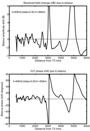
0 1000 2000 3000 4000 5000 6000 −4 −2 0 2 4 6 8

Received field change (dB) due to biteout

f=40kHz;beta=0.50,h’=80km 0 1000 2000 3000 4000 5000 6000 −80 −60 −40 −20 0 20 40 60 80

VLF phase shift due to biteout

Biteout phase shift (degrees)

Fig. 6. Change in subionospheric received VLF amplitude and phase due to biteout, at f =40 kHz. Amplitude shifts are not in-considerable at about −2 dB, with positive spikes at modal minima.

Phase shifts are variable and up to 10◦inside the first modal

mini-mum at 3000 km. At long range large shifts up to 80◦are indicated

with a preference for positive sign.

An alternative approach to the modelling of Trimpis was adopted in Poulsen et al. (1990, 1993). They based their computations on an expression due to Wait (1964) which assumes linear Born scattering and a large, slowly varying ionospheric perturbation, allowing one to neglect intermodal coupling in the scattering process. Given more data on the spatial distribution of a biteout, this approach could indeed be used to model the VLF perturbations due to a patchy bite-out of finite extent.

The rigorous solution to the problem would involve 3-D fi-nite element modelling at huge computational expense. Thus far only 2-D finite element codes have been developed for modelling subionospheric VLF propagation under an inho-mogeneous ionosphere (Baba and Hayakawa, 1996).

Perhaps an equally attractive approach to the problem of subionospheric VLF propagation under an inhomoge-neous ionosphere is to use a time domain FDTD integration (Berenger, 1994, 2002). While conceptually simpler than Fi-nite Element methods, nonetheless the computational load is high, and thus far only 2-D models have been developed.

The MODEFNDR code we employ here computes re-ceived Ezphase (relative to free space propagation) and

am-plitude as a function of range for the profile, with and with-out bitewith-out. We present the result as the change in

propa-gation amplitude and phase resulting from the biteout. These shifts of course apply equally well to the horizontal magnetic field components perpendicular to the direction of propaga-tion, namely Bx and By. It is these changes that are to be

the VLF diagnostic for electron density biteouts, and to the extent that biteout occurrence correlates with PMSE, they be-come diagnostics for PMSE.

3 Computed results for VLF propagation

3.1 Propagation at 20 kHz

Prior to examining the VLF amplitude and phase shifts due to biteouts, it is a useful exercise to examine the modal mix at each frequency, the parameters appertaining to each mode, and how they are shifted by the biteout.

Figure 2 displays the modal parameters at 20 kHz. The modes returned by MODEFNDR have been re-ordered with TM modes first followed by the TE modes. All modes whose contribution is entirely negligible at ranges between 500 and 6000 km have been ignored. The top left panel shows v/c, the wave phase velocity v=ω/k||relative to c. This is greater

than unity since cos θ ∼ c/v, where θ is the propaga-tion angle relative to horizontal at the reference height. The dashed blue curve (with x) represents the corresponding re-sult with biteout. Of the nonnegligible propagation modes found by the code, 5 are TM modes and 9 are TE modes. The higher order modes clearly have increasing propagation angles. The top right panel shows modal attenuation factor in dB/Mm. Attenuation increases to large values for higher order modes. The leading TE modes have low attenuation and may be important at long range. The bottom left panel shows |λ|, the absolute value of Wait’s excitation factors. As is well known, in the case of vertical electric dipole excita-tion, TM modes are strongly excited and TE modes weakly excited. The fourth panel estimates the relative modal mix at the minimum range of 500 km (black, solid, x; biteout blue, dashed, o) and the maximum range of 6000 km (red, solid, x; biteout green, dashed, x). Clearly at short range we have a very broad modal mix, with TM1–TM5 modes being of sig-nificance as well as TE10. At long range TM1 and TM2 and TE6 alone are significant.

Figure 3 plots the corresponding shifts in the modal pa-rameters due to biteout at 20 kHz. These are important since it is these shifts ultimately that give rise to the propagation perturbations. The parallel phase velocity is increased for TM modes but decreased for TE modes. Attenuation in-creases for TM modes but dein-creases for TE modes. There is a large increase in excitation for TM1, other TM modes being less excited. Low-order TE modes are more strongly excited, in particular making TE7 more significant at long range. The solution of the modal equation is highly complex and it is difficult to formulate simple explanations for these results. The fourth panel shows the shift in modal amplitude at ranges of 500 km (black) and 6000 km (green). The effect

(8)

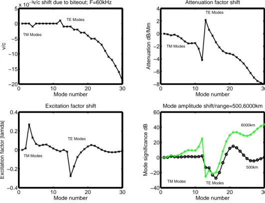
0 10 20 30 −20 −15 −10 −5 0 5x 10

−3 v/c shift due to biteout; F=60kHz

Mode number v/c TM Modes TE Modes 0 10 20 30 −8 −6 −4 −2 0 2 4

Mode number Attenuation dB/Mm TM Modes TE Modes 0 10 20 30 −0.4 −0.2 0 0.2 0.4

Mode number

TM Modes TE Modes 0 10 20 30 −40 −20 0 20 40 60

Mode number

500km 6000km

TM Modes _{TE Modes}

Fig. 7. Shift in modal parameters due to biteout at f =60 kHz. Key features are the decreased attenuation and increased excitation of TM modes and decreased phase velocity of TE modes.

of biteout is to raise the significance of TE6 and TE7, but reduce that of TM2–TM5.

Figure 4 plots the shift in VLF received amplitude (in dB) and phase at 20 kHz as a function of range. At ranges less than 2800 km, many modes are significant in the received signal and the resulting shift, though significant and in the region of 1–2 dB, is highly variable and unpredictable. The very large perturbations ∼±3 dB at 2800 km and 4400 km correspond to the location of modal interference minima. Be-yond 4000 km the general effect of biteout is a reduction of received amplitude by about 1 dB. Regarding received phase a similar pattern is observed, chaotic at short range, with sharp maxima at modal minima. At large ranges a coher-ent pattern emerges with phase advances in the region of 4◦_.

The behaviour at long range, where a few TM modes domi-nate, is consistent with our modal investigation. The negative amplitude change and positive phase shift is consistent with the dominant TM modes undergoing increased attenuation and phase velocity and decreased excitation factor. The in-creased excitation of TM1 is not enough to counteract this pattern.

It is interesting to note that VLF propagation perturbations at long ranges (∼6000 km), even assuming the biteout covers the whole GC corridor, are no larger than those calculated for short range. This suggests that experiments could be usefully set up using short paths only. In addition, this indicates that biteouts covering a significant fraction of the ∼6 Mm path will lead to similar changes as that determined, assuming the entire path has biteout conditions.

Figure 5 show the shifts in modal parameters due to biteout at 40 kHz. These are rather different due to different degrees of penetration of the modes to 85 km and the different corre-lations between the biteout and height gain function profiles. The shifts in parallel phase velocities are much smaller and negligible for the TM modes but substantially negative for TE modes. The dominant TM and TE modes have increased attenuation, the others having reduced attenuation. The dom-inant TM modes have reduced excitation.

Figure 6 plots the received VLF amplitude and phase shifts at 40 kHz. Inside the first modal interference minimum at 3000 km the shifts are irregular in the region of 10◦_{of phase}

and 1 dB. Beyond this range amplitude shift is in the re-gion of −2 dB, but becomes large and positive (∼8 dB) at the next minimum at 5000 km. Negative amplitude shifts are due to the increased attenuation and decreased excitation of the dominant TM modes. Phase shifts at ranges larger than 3000 km are substantial (∼40◦) but of unpredictable sign and are harder to interpret.

Figure 7 shows the modal parameter shifts at 60 kHz and in-dicates small negative changes in parallel phase velocity for TE modes, decreasing attenuation for the TM modes and TE modes, with the exception of the leading TE modes TE13 and TE14. Dominant TM modes TM3 and TM4 have a con-siderable increase in excitation factor. Figure 8 shows the

(9)

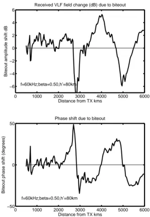
0 1000 2000 3000 4000 5000 6000 −6 −4 −2 0 2 4 6

Received VLF field change (dB) due to biteout

0 1000 2000 3000 4000 5000 6000 −50

0 50

Phase shift due to biteout

Fig. 8. Change in subionospheric received VLF amplitude and phase due to biteout, at f =60 kHz. The general trend is for a posi-tive shift, up to a substantial maximum of 5 dB, but with large neg-ative spikes at modal minima. Inside 3000 km the shift is between

0 and +2 dB. Phase shifts at large range seem to be ±20◦, with

smaller values up to about 8◦inside 2000 km.

VLF amplitude and phase shifts at 60 kHz. The former are generally positive and ∼2 dB inside the first modal minimum at 3000 km, which is due to decreased attenuation and in-creased excitation factors of the dominant TM modes. Phase shifts inside the first modal minimum are small ∼7◦ and of indeterminate sign. Beyond 3000 km amplitude and phase shifts are quite large (∼20◦, 4 dB) but can be of either sign depending on range.

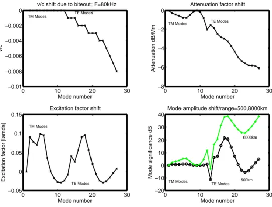
Figure 9 show the modal parameter shifts at 80 kHz. A fairly consistent pattern is seen, namely a decrease in parallel phase velocity in the case of TE modes, decreased attenuation for all modes and small increases in excitation factor. These changes are reflected in Fig. 10, showing propagation per-turbations at 80 kHz. The overall amplitude shift is positive and quite substantial in the range 1–4 dB. A strong negative peak from −2 to −6 dB stretching across the range 3100– 3400 km is seen in the region of the modal interference min-imum at 3200 km . There is a good deal of variability related to the multimodal character of the propagation. The phase shift is consistently negative at a substantial value ∼−20◦, except for a large positive peak at 2900 km. This is due in part to the decrease in parallel phase velocity for all modes.

4 Profile and frequency dependence of VLF

propaga-tion disturbances

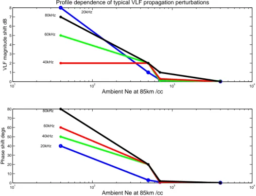
It is a matter of some interest and importance as to how the overall magnitude of VLF propagation amplitude and phase shift depend on unperturbed electron density profile and on frequency. During the course of this research numerous pro-files were investigated. It became clear that the perturba-tion size could be viewed as depending on the unperturbed ambient electron density at the biteout level of 85 km. We have selected four diverse profiles and plotted the mean abso-lute value of perturbation (both amplitude and phase) at long range, as a function of ambient density at 85 km. Figure 11 shows these results for all four frequencies. It is apparent that once the ambient electron number density at 85 km exceeds about 500 el/cc, the size of the perturbation of VLF propaga-tion collapses to negligible levels, due, of course, to shield-ing and the non penetration of the modal height gain func-tions to the biteout altitude of 85 km. Conversely, for pro-files with generally lower electron densities, associated with night/dusk/low solar elevation, VLF propagation changes be-come very large, for example, 8 dB and 80◦in one case.

Another matter of considerable interest is the frequency dependence of the size of the propagation disturbances. As far as phase shift is concerned, this seems to increase some-what with frequency (roughly as√f )for low density pro-files. The same may be said for the magnitude perturbation, except for 20 kHz, which has an anomalously large value. With denser profiles a clear frequency dependence is hard to discern, except that 20 kHz is here anomalously low, for both amplitude and phase perturbations. The dependence of modal parameters on profile is immensely complex, and these dependencies are presumably due to the extent to which each mode penetrates to the biteout altitude and the correla-tion of the biteout profile with the height gain funccorrela-tions.

Given the apparent upper limit of 500 el/cc for the pro-duction of significant signatures of biteouts in VLF signals we would expect preferred periods when they could be ob-served. We can estimate the electron number density levels at 85 km by using the solar zenith angle control of β and h0and fitting of the ionospheric profile through experimentally de-termined (empirical) relationships (Thomson, 1993; McRae and Thomson, 2000). Figure 12 shows the expected diurnal variation of the electron density at the summer solstice on 21 June for latitudes of 60, 65, and 70◦. The electron density is shown by the roughly sinusoidally varying line in this fig-ure. That section of the line marked by circles corresponds to the solar zenith angle range (<80◦₎_{over which the}

empir-ical expressions were developed. Beyond this area the elec-tron density values can only be considered approximate. The horizontal line indicates the cutoff level of 500 el/cc. Cal-culations for 21 July, one month after the summer solstice, gave a similar result. It can be seen that the VLF technique is potentially able to operate successfully for about 10 h per day, centred about midnight, during the arctic summer PMSE season. This estimate is confirmed by the quiet-time iono-sphere models for auroral latitudes developed by Friedrich

(10)

0 10 20 30 −0.01 −0.008 −0.006 −0.004 −0.002 0

v/c shift due to biteout; F=80kHz

Mode number v/c TM Modes TE Modes 0 10 20 30 −8 −6 −4 −2 0

Mode number Attenuation dB/Mm TM Modes TE Modes 0 10 20 30 −0.05 0 0.05 0.1 0.15

Mode number

TM Modes TE Modes 0 10 20 30 −20 −10 0 10 20 30 40

Mode number

Mode significance dB _500km

6000km

TM Modes _{TE Modes}

Fig. 9. Shift in modal parameters due to biteout at f =80 kHz. Key features are the decreased attenuation and increased excitation of TM modes and decreased phase velocity of TE modes.

et al. (2001) (Personal communication, R. Steiner, 2003). This empirical model suggests an observation window for our VLF technique of about 6 h at 60◦latitude and probably less at higher latitudes. Significant increases in background electron density at 85 km would be expected during any ge-omagnetic activity periods, which would result in the exclu-sion of the VLF wave from the biteout altitudes. Thus, quiet geomagnetic conditions would be a necessary condition to detect the VLF signature of large-scale biteouts.

5 Conclusions

We have determined that realistic “biteouts” of the elec-tron density profiles can cause observable changes in sub-ionospheric VLF propagation characteristics. These results were calculated under the assumption that the biteout cov-ers a 300 km corridor along the whole GC path. For ambient profiles, with densities ∼500 el/cc at 85 km, which is on the low side and associated more with the 10 h period about mid-night, perturbations were of the order of 1–2 dB and 10–20◦_.

The dependence of perturbation on range was quite erratic at relatively short ranges <2500 km, due to the multimodal na-ture of the propagation for these distances. At longer ranges a more settled pattern emerged, with negative amplitude and positive phase shift predominating at 20 kHz and the opposite at 80 kHz. The patterns at 40 and 60 kHz were less straight-forward. Perturbations are sharply dependent on ambient density at 85 km, quickly collapsing when density exceeds about 500 el/cc, but becoming large for lower densities.

0 1000 2000 3000 4000 5000 6000 −6 −4 −2 0 2 4 6

Received VLF field change (dB) due to biteout

f=80kHz;beta=0.50,h’=80km 0 1000 2000 3000 4000 5000 6000 −60 −40 −20 0 20 40 60

Phase shift due to biteout

Fig. 10. Change in subionospheric received VLF amplitude and phase due to biteout, at f =80 kHz. At this frequency the shift shows a complex pattern, and is mainly positive at a typical level of +2 dB.

A fairly consistent pattern of negative phase shifts ∼−20◦will be

(11)

101 102 103 104 0 1 2 3 4 5 6 7 8 VLF magnitude shift dB Ambient Ne at 85km /cc

Profile dependence of typical VLF propagation perturbations

20kHz 40kHz 60kHz 80kHz 101 102 103 104 0 10 20 30 40 50 60 70 80

Phase shift degs

Ambient Ne at 85km /cc

20kHz 40kHz

60kHz 80kHz

Fig. 11. Variation of the VLF amplitude and phase perturbations with frequency and ambient electron density at 85 km. We have utilised median values of the magnitudes of amplitude and phase perturbations at long range. Note the rapid increase as density decreases below 500 el/cc. Overall perturbation magnitude increases with frequency.

0 4 8 12 16 20 24 101

102 103 104

Electron Density 85km altitude (el./cc)

UT 60N

21 June

65N 70N

Fig. 12. Estimated electron density at 85 km at the summer solstice (21 June) as a function of universal time at 60, 65, 70 N and at zero longitude. Below the horizontal line at 500 el/cc we expect feasible VLF detection of electron density biteouts.

Taking a global view, the VLF perturbations increased some-what with frequency.

Thus, as a means of detecting Biteouts/PMSE, VLF prop-agation would appear to be effective when ambient densities at 85 km are less than 500 el/cc. This is precisely the domain where PMSEs are not reported in radar data, and thus, VLF may be the basis of a valuable complimentary measurement technique.

This research suggests experimental programs in which trans-arctic VLF propagation paths are selected and VLF propagation in summer is closely monitored and compared with the incidence of observed PMSE and noctilucent clouds, or indeed direct rocket observations of biteout. As a diag-nostic, VLF propagation shifts will be a measure of the inte-grated effect of an electron density biteout along a GC corri-dor, connecting a given transmitter and receiver, in contrast to rocket/PMSE measurements which are essentially point measurements. A key factor here will be the stability of the VLF propagation. One will be observing shifts in VLF am-plitude and phase as biteouts develop along or move through the GC corridor. The detectability of these shifts will in part depend upon the typical time signature of the VLF propaga-tion shifts and how they compare with the time signatures of all the other causes of VLF propagation variability. Certainly use of multiple frequencies and multiple paths can only im-prove the probability of biteout detection and/or reduce the false alarm rate. Observations can reasonably be confined to periods when the ambient profile is known to be “weak”,

(12)

i.e. under quiet magnetic conditions and around midnight. In this regard it would also appear to be beneficial to site the receiver close to a multimodal interference minimum.

Regarding future work such experiments would require further modelling for specified paths, in which the depen-dence of VLF perturbations on biteout altitude and depth was investigated. The problem of modelling biteouts with a patchy horizontal distribution remains difficult. If one can assume weak Born scattering and negligible intermodal cou-pling, as well as a homogeneous background ionosphere, the use of the formalism in Wait (1964) would certainly provide a solution. A more rigorous treatment would require 3-D FDTD codes or 3-D finite element codes, through the future development of existing 2-D codes (Baba and Hayakawa, 1996). In addition, further knowledge on the characteristics of biteouts are required in order for more realistic calcula-tions to be made. Some information may be gained by the joint deployment of radar and VLF observational systems in campaign environments.

Acknowledgements. The authors wish to thank NOSC, San Diego,

for permission to use the MODEFNDR software.

Topical editor U.-P. Hoppe thanks a referee for his help in eval-uating this paper.

References

Baba, K. and Hayakawa, M.: Computational results of the effect of localised ionospheric perturbations on subionospheric VLF prop-agation, J. Geophys. Res., 101, A5, 10 985–10 993, 1996. Barr, R., Jones, D. L., and Rodger, C. J.: ELF and VLF Radio

Waves, J. Atmos. Sol. Terr. Phys., 62, 17–18, 1689–1718, 2000. Berenger, J. P.: A perfectly matched layer for the absorption of

electromagnetic-waves, J. Comput. Phys., 114, 185–200, 1994. Berenger, J. P.: FDTD computation of VLF-LF propagation in

the Earth-ionosphere waveguide, Ann. Telecommun., 57, 1059– 1090, 2002.

Bickel, J. E., Ferguson, J. A., and Stanley, G. V.: Experimental ob-servation of magnetic field effects on VLF propagation at night, Radio Science, 5, 19, 1970.

Blix, T., Rapp, M., L¨ubken, F.-J.: Relations between small-scale electron number density fluctuations, radar backscatter, and charged aerosol particles, J. Geophys. Res., 108, D8, 8450, 2003. Bremer, J., Singer, W., Keuer, D., Hoffman, P., Rottger, J., Cho, J. Y. N., and Schwartz, W. E.: Observations of Polar Mesospheric Summer Echoes at EISCAT during Summer 1991, Radio Sci-ence, 30, 4, 1219–1228, 1995.

Bremer, J., Hoffman, P., Singer, W., Meek, C. E., and Ruster, R.: Simultaneous PMSE Observations with ALOMAR-SOUSY and EISCAT-VHF Radar During the ECHO-94 Campaign, Geophys-ical Research Letters, 23, 10, 1075–1078, 1996.

Bremer J., Hoffmann, P., Latteck, R., and Singer, W.: Seasonal and long-term variations of PMSE from VHF radar observations at Andenes, Norway, J. Geophysical Research-Atmospheres, 108 (D8): art. no. 8438, Feb 8, 2003.

Cho, J. Y. N. and Rottger, P.: An Updated Review of Polar Meso-sphere Summer Echoes: Observation, Theory, and their Rela-tionship to Noctilucent Clouds and Subvisible Aerosols, J. Geo-phys. Res., 102, D2, 2001–2020, 1997.

Croskey, C. L., Mitchell, J. D., Friedrich, M., Torkar, K. M., Hoppe, U.-P., and Goldberg, R. A.: Electrical Structure of PMSE and NLC Regions during the DROPPS Program, Geophysical Res. Letters, 28, 8, 1427–1430, 2001.

Deshpande, S. D. and Mitra, A. P.: Ionospheric effects of solar flares IV, Electron density profiles deduced from measurements of SCNA’s and VLF phase and amplitude, J. Atmos. Terr. Phys., 34, 255–266, 1972.

Ferguson, J. A. and Snyder, F. P.: Computer Programs for As-sessment of Long Wavelength Radio Communications, Naval Oceans Systems Centre Technical Document 1773, 1990. Friedrich, M. and Kirkwood, S.: The D-region background at high

latitudes, Adv. Space Res., 25, 1, 15–23, 1999.

Friedrich, M., Torkar, K. M., Harrich, M., Pilgram, R., and Kirk-wood, S.: On merging empirical models for the lower ionosphere of auroral and non-auroral latitudes, Adv. Space Res., 29, 6, 929– 935, 2002.

Goldberg, R. A., Pfaff, R. F., Holzworth, R. H., et al.: DROPPS: A study of the Polar Summer Mesosphere with Rocket, Radar and Lidar, Geophysical Res. Letters, 28, 8, 1407–1410, 2001. Hardman, S., Rodger, C. J., Dowden, R. L., and Brundell, J. B.:

Measurements of the VLF scatter pattern of the structured plasma of red sprites, IEEE Antennas Propag. Mag., 40, 29–38, 1998. Helliwell, R. A., Katsufrakis, J. P., and Trimpi, M. L.:

Whistler-induced amplitude perturbation in VLF propagation, J. Geophys. Res., 78, 4679–4688, 1973.

Helliwell, R. A.: VLF wave stimulation experiments in the mag-netosphere from Siple Station, Antarctica, Rev. Geophys., 26, 3, 551–578, 1988.

Hoppe, U.-P., Blix, T. A., Thrane, E. V., Lubken, F. J., Cho, J. Y. N., and Schwartz, W. E.: Studies of Polar Mesospheric Summer Echoes by VHF Radar and Rocket Probes, Adv. Space Res., 14, 9, 9139–9148, 1994.

McRae, W. M. and Thomson, N. R.: VLF phase and amplitude: daytime ionospheric parameters, J. Atmos. Sol. Terr. Phys., 62, 7, 609–618, 2000.

Morfitt, D. G. and Shellman, C. H.: MODESRCH, an Improved Computer Program for Obtaining ELF/VLF/LF Mode Constants, Naval Electronics Lab Centre Interim Report 771, NTIS Acces-sion No. ADA032573, National Technical Information Service, Va. 22161, USA, 1976.

Murphy, D. J. and Vincent, R. A.: Amplitude Enhancements in Antarctic MF Radar Echoes, J. Geophys. Res., 105, D21, 26 683–26 693, 2000.

Nunn, D.: On the Numerical modelling of the VLF Trimpi Effect, J. of Atmospheric and Terrestrial Phys., 59, 5, 537–560, 1997. Nunn, D. and Strangeways, H. J.: Trimpi Perturbations from Large

ionisation Enhancement Patches, J. of Atmospheric and Solar-Terrestrial Phys., 62, 189–206, 2000.

Palmer, J. R., Rishbeth, H., Jones, G. O. L., and Williams, P. J. S.: A Statistical Study of Polar Mesospheric Summer Echoes observed by EISCAT, J. Atmospheric and Terrestrial Physics, 58, 1–4, 307–315, 1996.

Pappert, R. A. and Hitney, L.R.: Empirical modeling of nighttime easterly and westerly VLF propagation in the Earth-ionosphere waveguide. Radio Sci., 23, 599–611, 1988.

Pfaff R., Holzworth, R., Goldberg, R., Freudenreich, H., Voss, H., Croskey, C., Mitchell, J., Gumbel, J., Bounds, S., Singer, W., and Latteck, R.: Rocket probe observations of electric field irregular-ities in the polar summer mesosphere, Geophys. Res. Letters, 28, 8, 1431–1434, 2001.

(13)

Poulsen, W. L., Bell, T. F., and Inan, U. S.: Three dimensional modelling of subionospheric VLF propagation in the presence of localised D-region perturbations associated with lightning, J. Geophys. Res., 95, 3, 2355–2366, 1990.

Poulsen, W. L., Inan, U. S., and Bell, T. F.: A Multiple Mode Three Dimensional Model of VLF Propagation in the Earth ionosphere Waveguide in the Presence of Localised D-Region Disturbances, J. Geophysical Res., 98, A2, 1705–1717, 1993.

Rapp, M., Gumbel, J., Lubken, F. J., and Latteck, R.: D-Region Electron Number Density limits for the Existence of Polar Meso-spheric Summer Echoes, J. Geophys. Res., 107, 14, 4187, 2002. Rodger, C. J. and Nunn, D.: VLF Scattering from Red Sprites, Ap-plication of Numerical Modelling, Radio Science, 34, 4, 923– 932, 1999.

Rodger, C. J.: Subionospheric VLF perturbations associated with lightning discharges, J. Atmos. Sol. Terr. Phys., 65, 591–606, 2003.

Taylor, M. J., Vaneyken, A. P., Rishbeth, H., Witt, G., Witt, N., and Clilverd, M. A.: Simultaneous observations of noctilucent clouds and polar mesospheric radar echoes – evidence of non-correlation, Planetary and Space Science, 37, 8, 1013–1020, 1989.

Thomas, G. E.: Mesospheric Clouds and the Physics of the

Mesopause Region, Rev. Geophys., 29, 4, 553–575, 1991. Thomson, N. R.: Experimental daytime VLF ionospheric

parame-ters, J. Atmos. Terr. Phys., 55, 173–184, 1993.

Ulwick, J. C., Baker, K. D., Kelley, M. C., Balsley, B. B., and Eck-lund, W. L.: Comparison of Simultaneous MST Radar and Elec-tron Density probe Measurements during STATE, J. Geophys. Res., 93, 6989–7000, 1988.

Wait, J. R.: Influence of a Circular Ionospheric Depression on VLF Propagation, Radio Science, 68, D8, 907–914, 1964.

Wait, J. R.: Electromagnetic Waves in Stratified Media, corrected reprinting of 1962 edition, IEEE Press, New York, 1996. Wait, J. R. and Spies, K. P.: Characteristics of the Earth-ionosphere