HAL Id: hal-00680921
https://hal.archives-ouvertes.fr/hal-00680921
Submitted on 22 Nov 2020
HAL is a multi-disciplinary open access
archive for the deposit and dissemination of
sci-entific research documents, whether they are
pub-lished or not. The documents may come from
teaching and research institutions in France or
abroad, or from public or private research centers.
L’archive ouverte pluridisciplinaire HAL, est
destinée au dépôt et à la diffusion de documents
scientifiques de niveau recherche, publiés ou non,
émanant des établissements d’enseignement et de
recherche français ou étrangers, des laboratoires
publics ou privés.
Infrared Radiometer. Part I: effective emissivity and
optical depth
Anne Garnier, Jacques Pelon, Philippe Dubuisson, Michaël Faivre, Olivier
Chomette, Nicolas Pascal, David P. Kratz
To cite this version:
Anne Garnier, Jacques Pelon, Philippe Dubuisson, Michaël Faivre, Olivier Chomette, et al.. Retrieval
of cloud properties using CALIPSO Imaging Infrared Radiometer. Part I: effective emissivity and
optical depth. Journal of Applied Meteorology and Climatology, American Meteorological Society,
2012, 51 (7), pp.1407-1425. �10.1175/JAMC-D-11-0220.1�. �hal-00680921�
Retrieval of Cloud Properties Using CALIPSO Imaging Infrared Radiometer. Part I:
Effective Emissivity and Optical Depth
ANNEGARNIER,* JACQUESPELON,* PHILIPPEDUBUISSON,1MICHAE¨ LFAIVRE,* OLIVIERCHOMETTE,#NICOLASPASCAL,@ANDDAVIDP. KRATZ& * Laboratoire Atmosphe`res, Milieux, Observations Spatiales, UPMC-UVSQ-CNRS, Paris, France
1Laboratoire d’Optique Atmosphe´rique, Universite´ de Lille 1, Lille, France #Laboratoire de Me´te´orologie Dynamique, Ecole Polytechnique, Palaiseau, France
@Hygeos, Lille, France
&NASA Langley Research Center, Hampton, Virginia
(Manuscript received 13 October 2011, in final form 23 February 2012) ABSTRACT
The paper describes the operational analysis of the Imaging Infrared Radiometer (IIR) data, which have been collected in the framework of the Cloud–Aerosol Lidar and Infrared Pathfinder Satellite Observation (CALIPSO) mission for the purpose of retrieving high-altitude (above 7 km) cloud effective emissivity and optical depth that can be used in synergy with the vertically resolved Cloud–Aerosol Lidar with Orthogonal Polarization (CALIOP) collocated observations. After an IIR scene classification is built under the CALIOP track, the analysis is applied to features detected by CALIOP when found alone in the atmospheric column or when CALIOP identifies an opaque layer underneath. The fast-calculation radiative transfer (FASRAD) model fed by ancillary meteorological and surface data is used to compute the different components involved in the effective emissivity retrievals under the CALIOP track. The track analysis is extended to the IIR swath using homogeneity criteria that are based on radiative equivalence. The effective optical depth at 12.05 mm is shown to be a good proxy for about one-half of the cloud optical depth, allowing direct comparisons with other databases in the visible spectrum. A step-by-step quantitative sensitivity and performance analysis is pro-vided. The method is validated through comparisons of collocated IIR and CALIOP optical depths for el-evated single-layered semitransparent cirrus clouds, showing excellent agreement (within 20%) for values ranging from 1 down to 0.05. Uncertainties have been determined from the identified error sources. The optical depth distribution of semitransparent clouds is found to have a nearly exponential shape with a mean value of about 0.5–0.6.
1. Introduction
The retrieval of cloud and aerosol radiative properties at the global scale is an important challenge for the understanding and surveying of climate change. In this respect, upper-level clouds are of particular interest since their microphysical characteristics are still poorly known despite their significant impact on the Earth radiation budget (Stephens et al. 1990; Kristja´nsson et al. 2000). The Cloud–Aerosol Lidar and Infrared Pathfinder Satel-lite Observation (CALIPSO) mission has been defined to allow a better understanding of aerosol and cloud radiative
forcing. Observations from the three-channel Imaging Infrared Radiometer (IIR) developed in France by the Centre National d’Etudes Spatiales (CNES), the Socie´te´ d’Etudes et de Re´alisations Nucle´aires (SODERN), and the Institut Pierre-Simon Laplace (IPSL) are com-bined with those from the Cloud–Aerosol Lidar with Orthogonal Polarization (CALIOP) to provide a new characterization of the microphysics at global scale using an improved split-window technique.
The split-window technique has long been applied to the data of spaceborne passive thermal imagers to retrieve the effective diameter of ice crystals in high-altitude clouds using two or three infrared channels (Inoue 1985; Ackerman et al. 1990; Giraud et al. 1997; Duda et al. 1998; Heidinger et al. 2010). Improvements have also been proposed that will take advantage of high-resolution infrared soundings and more sophisticated
Corresponding author address: Anne Garnier, LATMOS, Boıˆte 102, Universite´ Pierre et Marie Curie, 4 place Jussieu, 75252 Paris CEDEX 05, France.
E-mail: [email protected] DOI: 10.1175/JAMC-D-11-0220.1 Ó 2012 American Meteorological Society
radiative transfer calculations (Ackerman et al. 1995; Ra¨del et al. 2003; Kahn et al. 2004; Pavolonis 2010; Stubenrauch et al. 2006; Wang et al. 2011; Wei et al. 2004; Yue et al. 2007). In the framework of the CALIPSO mission, we have chosen to use selected range-resolved lidar inputs in a standard split-window technique to provide a fast retrieval of cirrus optical (emissivity and optical depth) and microphysical (particle size and ice water path) properties taking into account critical vertical information (Cooper et al. 2003). The ice cloud micro-physical properties are derived from two micromicro-physical indices, defined as the ratio of the effective infrared optical depths in the two pairs of channels 10.6–12.05 mm and 8.65–12.05 mm, which are used to minimize the sensitivity to unknown parameters (Parol et al. 1991). This method, which is based on the retrieval of the cloud effective emissivities in the three IIR channels, also takes advantage of the different absorption by water and ice in those channels (Ackerman et al. 1990, 1995). Simulations have been performed using the Fast Discrete Ordinate Method (FASDOM) radiative transfer model (Dubuisson et al. 2008), theoretical optical properties of several complex crystals (Yang et al. 2005), and using various ancillary atmospheric and surface parameters to define lookup tables to further retrieve the effective size of the cirrus ice crystals for a preferred shape from the two microphysical indices.
This paper aims to present the first part of the algorithm dedicated to IIR cloud effective emissivity and optical depth retrievals whereas microphysical properties will be the topic of a future publication. The basics of the IIR algorithm are presented in section 2. The track analysis including the CALIOP-based scene classification is de-tailed in section 3, and the IIR swath analysis is in section 4. Section 5 is devoted to the optical depth retrievals. Section 6 discusses the sensitivity to the key parameters and associated uncertainties. Results are shown and dis-cussed in section 7 before ending with the conclusions.
2. Analysis method
The IIR instrument consists of three window channel spectral bands centered at 8.65, 10.6, and 12.05 mm that have medium spectral resolution of respectively 0.9, 0.6, and 1 mm but that exclude the ozone absorption band centered at 9.6 mm. The sensor is an uncooled micro-bolometer offering a compromise between intrinsic noise (Table 1) and reachable performance, mainly controlled by the accuracy on ancillary parameters used in the inversion scheme. The objective is to implement a split-window technique involving the three IIR chan-nels improved by identifying the relevant conditions based on the vertical information available from the
CALIOP collocated observations under the satellite track. The overall scheme of the method is described through the flow diagram shown in Fig. 1. Level 1 calibrated and geolocated IIR radiances, measured in a near-nadir viewing geometry, are registered on a refer-ence grid centered on the CALIOP ground track, with 1-km horizontal resolution over a 69-1-km swath. In the same manner, the daytime level 1 wide field camera (WFC) reflectance at 0.62–0.67 mm is available on the same grid as the IIR as an input of the algorithm.
To take advantage of the sensitivity of the aerosols and cloud detection provided by the CALIOP data analysis (Vaughan et al. 2009), the IIR scene classification is based on the CALIOP 5-km Cloud and Aerosols Layer products (currently version 3 products). Aerosol layers are included to account for polar stratospheric clouds reported in this product and for particles such as mineral dust or compo-nents of volcanic plumes absorbing in the thermal infrared. Each observational area is 5 km along the satellite track and 100 m wide across the track because of the size of the laser spot near the earth’s surface, and coincides with five successive 1-km IIR pixels. Although IIR observa-tions are available at 1-km resolution, the CALIOP 1-km-layer products are presently not used because they do not report thin layers detected at a coarser resolution (5, 20, or 80 km) in the 5-km products (Vaughan et al. 2009). Thus, identical CALIOP parameters over five consecutive pixels are presently used in the 1-km IIR analysis, slightly increasing the retrieval uncertainty.
The IIR scene classification is built to select the suit-able scenes for the track analysis. The effective emissivi-ties are computed for each IIR pixel under the lidar track, for each IIR channel separately, with the same algorithm for daytime and nighttime measurements, at any latitude over land and ocean. Furthermore, as the IIR window channels basically sense the surface and the lowermost atmosphere, the algorithm corrects the observed radi-ances for the so-called background radiance that would be observed in the absence of the studied cloud. CALIOP vertical information allows one to select useful reference observations if any. Otherwise, the correction relies on the fast-calculation radiative transfer (FASRAD) model (Dubuisson et al. 2005) provided with the required ancil-lary products, namely surface type and surface temperature
TABLE1. Radiometric performance of the IIR microbolometer measured before launch.
NedT 1 sigma value
(83% of pixels) 8.65 mm 10.6 mm 12.05 mm @210 K 0.20 K 0.27 K 0.19 K @250 K 0.09 K 0.14 K 0.11 K
together with the temperature, water vapor, and ozone atmospheric profiles. Effective infrared optical depths are then inferred from the effective emissivity retrieved in each IIR channel.
The scene classification, effective emissivities, and optical depths are spread to the IIR swath through homogeneity criteria involving the three IIR radiances and possibly the daytime WFC reflectance, as will be discussed in section 4. The track and swath parameters are reported in the respective IIR level 2 products (currently version 3).
3. Track analysis a. Scene classification
The IIR level 2 algorithm uses the CALIOP 5-km Cloud and Aerosols Layer operational products to build a scene classification designed to select the scenes to be further analyzed. In the CALIOP operational algorithm, the layers are detected using the level 1 532-nm total at-tenuated backscatter (Vaughan et al. 2009), which are further classified as clouds or aerosols (Liu et al. 2009). Each layer is located vertically with a resolution of 30 m from the ground to 8.2 km, then 60 m from 8.2 to 20.2 km, and finally 180 m from 20.2 to 30.1 km. The horizontal resolution is defined by the amount of aver-aging required to detect the layers. We choose to consider only the layers detected with 5- and 20-km horizontal averaging as the latter resolution corresponds to emis-sivities of the order of magnitude of the IIR sensitivity. Indeed, according to Vaughan et al. (2009), the features detected with 20-km horizontal averaging have integrat-ed backscatter intensities mostly between 4 3 1024and 2 3 1023sr21, corresponding to a visible optical depth between 0.01 and 0.05 assuming a lidar ratio of 25 sr for ice as used in the CALIOP operational algorithm, and
thus to emissivities of roughly half of these values as will be discussed in section 5.
The IIR classification is built from the number of scat-tering layers, their altitudes, cloud–aerosols classification, mean volume depolarization ratio, and the opacity flag of the lowermost layer as identified from CALIOP data. The scenes are sorted following the number of semi-transparent layers defined as high when their centroid altitude is above 7 km, or low otherwise. Two main cate-gories are defined based on the background scene, which can be either the surface if the lowermost layer is not opaque or a dense opaque layer, corresponding to two different modes to compute the effective emissivities. We focus here on the main objectives of the IIR observations, which are the characterization of ice cloud properties. This mostly involves scenes containing a single-layer semi-transparent cloud (STC) overlying either the surface (type 21) or a dense opaque layer (type 31) and scenes con-taining 1 high dense cloud (type 40) (Table 2). When a single-layer STC is found, the algorithm checks for the
FIG. 1. The IIR level 2 algorithm flow diagram.
TABLE2. IIR scene classification for high-altitude clouds (.7 km). Scene Target description Reference
21 1 high STC layer and no aerosol layer
Surface 30 1 high STC layer and
nondepolarizing aerosols
Surface 40 1 high opaque cloud layer,
vol_depol_ratio_max . 40%
Surface 80 1 high opaque cloud layer,
vol_depol_ratio_max , 40%
Surface 22 2 high STC layers Surface 26 3 high STC layers Surface
31 1 high STC layer Low opaque cloud 32 2–5 high STC layers Low opaque cloud 37 1 high STC layer Low opaque aerosol 41 1 high STC layer High opaque cloud 42 2 high STC layers High opaque cloud
detection of aerosol layers and labels the scene ac-cordingly (type 30). Low-altitude aerosol layers are split according to the mean volume depolarization ratio in the layer, with a threshold of 6% to identify more-depolarizing semidesert aerosols (Liu et al. 2008). Over-all, about 40 types of scenes are identified (list available at http://eosweb.larc.nasa.gov/PRODOCS/calipso/Quality_ Summaries/CAL_IIR_L2_Track_3-01.html). As an illus-tration, Fig. 2 shows a level 1 CALIOP quick-look (Fig. 2a) and the corresponding classification (Fig. 2b), where scenes of type 21, 30, and 40 are identified. The swath classification is presented in section 4.
b. Effective emissivities
The analysis is first applied to the IIR pixels collocated with the lidar track for the types of scenes identified in the scene classification module. This provides the effective emissivity at 8.65, 10.60, and 12.05 mm of the upper cloud or aerosol layer(s) constituting the so-called target. The effective emissivity refers to the contribution of scattering in the retrieved emissivity, especially in the 8.65-mm IIR channel in the case of small ice crystals. Effective emissivity could refer also to the unknown fractional cloud
cover in the IIR pixels as the lidar observational area covers only 10% of the 1-km IIR track pixels in the cross-track direction. However, we assumed that each pixel has a fractional cloud cover of 1 or 0 (Parol et al. 1991).
For each spectral channel k, centered on the wave-length lk, the track effective emissivity «effk of a
semi-transparent feature located at the reference altitude Zc
has been defined to be consistent with early works (Allen 1971; Platt and Gambling 1971):
«eff
k 5(Rk2RkBG)/[Bk(Tc, Zc) 2 RkBG]. (1)
In Eq. (1), Rk is the calibrated radiance measured
in channel k. The quantity Rk
BG
is the background radiance, that is, the outgoing top-of-the-atmosphere (TOA) radiance that would be observed in the absence of the studied cloud. Finally, Bk(Tc, Zc) is the opaque
cloud radiance, that is, the radiance of a blackbody source located at the reference altitude Zcof
thermo-dynamic temperature Tcretrieved from ancillary
mete-orological data. The retrievals are not attempted if Bk(Tc, Zc) is found to be equal to RkBG.
FIG. 2. (a) Example of lidar cross section, (b) related IIR cloud classification over the track (see Table 2), (c) classification extended to the swath, and (d) brightness temperature at 12.05 mm over the swath.
1) DETERMINATION OF THE BACKGROUND RADIANCE
Two approaches are available to derive the back-ground radiance. The primary approach is based on measurements in neighboring pixels while the alterna-tive is based on modeling.
The background radiance Rk
BG
is preferably de-termined from observations in neighboring pixels at a distance chosen to be less than 100 km from the ana-lyzed pixel, assuming an atmospheric homogeneity within a few kelvins. If the reference is the surface, the rele-vant neighboring pixels are those labeled as ‘‘clear sky’’ by the scene classification module and of same surface type (see following paragraph) than the ana-lyzed pixel. If the reference is an opaque layer, the permitted altitude difference is 6100 m, correspond-ing to a maximum difference of 61 K assumcorrespond-ing a 10 K km21adiabatic lapse rate.
If these spatial conditions are not satisfied, the back-ground radiance is computed using the FASRAD model (Dubuisson et al. 2005) adapted to the IIR spectral func-tions. This model is systematically run for a posteriori comparisons with the observations (see section 6). FASRAD is fed by the following ancillary data available to the CALIPSO project: (i) temperature, specific humidity, ozone profiles from the Global Modeling Assimilation Office (GMAO) Goddard Earth Observing System Model, version 5 (GEOS5) (G5.1.0 until August 2008 and G5.2.0 afterward), sampled every 6 h on a global2/38 3½8
longitude 3 latitude horizontal grid, (ii) GMAO GEOS5 surface temperature every 3 h and on a global2/38 3½8
longitude 3 latitude horizontal grid, and (iii) surface types from the International Geosphere and Biosphere Program (IGBP) daily updated according to the Near-Real-Time Ice and Snow Extent (NISE) 25-km product of the National Snow and Ice Data Center (NSIDC). CALIPSO uses the same surface types as those used in the Clouds and the Earth’s Radiant Energy System/Surface and Atmospheric Radiation Budget (CERES/SARB) map reported with a 109 resolution and the NISE data remapped by CERES onto a 10-min grid (cf. http://www-calipso.larc.nasa.gov/products/CALIPSO_DPC_Rev3x3. pdf). Surface emissivities are inferred from IGBP–NSIDC surface type, and averaged values are recalculated in the IIR bands from laboratory measurements following pro-cedures defined by the CERES team (Wilber et al. 1999). They are reported in Table 3.
2) DETERMINATION OF THE BLACKBODY RADIANCE
The cloud reference altitude Zcis a matter of
impor-tance, and although we agree that this term should be
considered the effective altitude for the contributed ra-diation (Cooper et al. 2003) no unique solution is proposed. Instead, it has been defined as the mean height of the cloud (Platt and Gambling 1971). The cloud temperature Tc has also been defined as the
brightness temperature of dense cloud tops detected in the same spectral domain (Inoue 1985; Parol et al. 1991; Giraud et al. 1997). Cloud properties derived from multichannel spectral analyses have also been used (Ra¨del et al. 2003; Wei et al. 2004). In this anal-ysis, we use the characterization of the feature back-scatter intensity provided in the CALIOP layer products. The altitude Zc is chosen as the centroid
altitude (Vaughan et al. 2005), defined as
Zc5
å
i51,N TR2ibetaiziå
i51,N TR2ibetai , (2)where the summations are taken over the N bin ranges located between the top and the bottom of the scattering feature. For each bin range i, ziis the altitude and TR2i is
the 2-way transmission at 532 nm between the top of the atmosphere and the bin range corrected from the atten-uation due to air molecules and ozone. Betaiis the total
backscatter coefficient at 532 nm. Assuming a linear re-lationship between altitude and temperature, the cloud thermodynamic temperature Tcderived from the centroid
altitude is related to the thermodynamic temperature Ti
in each bin i as
TABLE3. IIR surface emissivities. IIR channel 1 8.2–9.1 IIR channel 2 10.3–10.9 IIR channel 3 11.55–12.55 IGBP surface 0.9904 0.9888 0.9909 (1) evergreen needleleaf 0.9904 0.9888 0.9909 (2) evergreen broadleaf 0.9775 0.9738 0.9733 (3) deciduous needleleaf 0.9775 0.9738 0.9733 (4) deciduous broadleaf 0.9839 0.9813 0.9821 (5) mixed forests 0.9478 0.9653 0.9685 (6) closed shrublands 0.8754 0.9332 0.9411 (7) open shrublands 0.9801 0.9812 0.9886 (8) woody savannas 0.9801 0.9812 0.9886 (9) savannas 0.9801 0.9812 0.9886 (10) grasslands 0.9819 0.9857 0.9871 (11) permanent wetlands 0.9801 0.9812 0.9886 (12) croplands 1.0000 1.0000 1.0000 (13) urban 0.9820 0.9812 0.9854 (14) mosaic 0.9951 0.9967 0.9854 (15) snow/ice 0.8392 0.9171 0.9275 (16) barren/sparsely vegetated 0.9838 0.9903 0.9857 (17) water 0.9753 0.9936 0.9909 (18) tundra
Tc5
å
i51,N TR2ibetaiTiå
i51,N TR2ibetai . (3)The IIR algorithm selects a high-altitude cloud structure that is composed of one to a few layers. When more than one layer is found, the principle described above is upscaled to the cloud structure with the computation of the cloud structure centroid altitude and thermody-namic temperature.
Although CALIOP provides an accurate vertical description of the cloud, the cloud temperature Tcderived
from Eq. (3) is a priori, and thus may not be the correct equivalent radiative temperature of the cloud. Indeed, CALIOP observations report backscatter coefficients attenuated in a 2-way nadir viewing geometry in the vis-ible spectrum region. On the other hand, measurements in the IIR channels at the top of the atmosphere basically reflect the radiance of the surface further modified by the succession of overlying absorbing and emitting features. The impact of the difference between Tcused in this
al-gorithm and the true equivalent radiative temperature is estimated in section 6.
4. Extension to the swath
The lidar vertical information allows one to establish a detailed scene classification for IIR track pixels col-located with the lidar track. The analysis is extended to the 69-km IIR swath by attributing to each swath pixel outside the track the same type of scene and the same effective emissivity as the radiatively most similar neighboring track pixel. The corresponding pixel is quan-titatively identified at a maximum distance Vd from the closest track pixel through a homogeneity index (Hi) defined by averaging the absolute brightness tempera-ture differences for a given IIR channel (Hi 51 corre-sponds to a mean difference of 1 K). For each swath pixel, the most similar track pixel is the one providing the smallest Hi. A disadvantage of this approach is that a type of scene observed in the IIR swath, but not on the lidar track, cannot be categorized. This represents about 8% on average. Surface and atmospheric variations are not accounted for because the corresponding grids are presently of a few tens of kilometers. The WFC re-flectance is currently not used to avoid introducing a bias between night and day retrievals. Results for the ex-ample previously considered (Figs. 2a,b) are reported in Fig. 2c, showing the homogeneity of the mask obtained and the consistency with the corresponding brightness temperature (Fig. 2d). The white areas are where the swath categorization could not be made.
To validate the approach and to define the Hi index range and the distance Vd for the analyses, simulations were performed under the lidar track using the retrieved information. Figure 3a shows the distribution of the minimum Hi found within a distance Vd 5 50 km from each pixel identified as a single-layer high-altitude STC (type 21) for 120 full orbits in January 2011 between 608N and 608S. The simulations are restricted to areas of homogeneous surface emissivities within 1%. The cumu-lative occurrence distribution is plotted in red. The inside frame represents the distribution of the corresponding distances within the search area. The minimum Hi is smaller than 0.5 (K) in 85% of the cases and 1 (K) in 95% of the cases. The most similar pixels, that is, the smallest Hi indices, are found preferentially at a short distance from the reference pixels, between 1 km (op-timal distance) and 10 km, but can be found as far as 50 km for extreme swath pixels. When the distance is limited to 20 km, instead of 50 km, the homogeneity index stays smaller than 1 (K) in 95% of the cases. On the other hand, when Vd is limited to 20–50 km to simulate swath pixels located in the outer part of the IIR swath (Fig. 3b), the most similar pixels are found with similar probability levels at any distance within the search distance. The minimum Hi index is smaller than 1 (K) in 85% of the cases. On the basis of these simu-lations, we see that selecting a Hi index smaller than 1 (K) and a maximum distance Vd 5 50 km defines a reason-able trade-off between an acceptreason-able accuracy of the method and the wish to extend the classification to a sig-nificant part of the IIR swath. An Hi index smaller than 1 (K) for the accepted mean brightness temperature dif-ferences ensures effective emissivity difdif-ferences for swath pixels of the same order as the expected errors in the track emissivity retrievals, as discussed in section 6.
The accuracy of the method can be further evaluated by applying the swath extension algorithm to the track pixels for the main high cloud targets and by comparing the retrieved classification and effective emissivities with the actual track retrievals. As an illustration, we show the results obtained for type 21 scenes and Vd between 1 and 50 km for the same orbits of January 2011. The distribu-tion of the track scenes retrieved (Fig. 3c) shows that the swath algorithm is accurate for 72% of the cases, when the scene is also identified as type 21 under the track. Other types such as 30 (1 high layer with aerosols) and 23 (1 high layer with 1 low STC) represent 6% of the misclas-sifications, whereas types 31 (1 high layer with low opaque cloud) represent 1%. Types 22 (2 high layers) and 26 (3 high layers) represent 4% and less than 1%, respectively. High dense clouds (type 40) represent only 2%. Fur-thermore, 4% of the misclassifications correspond to clear sky (type 10), when the high-altitude cloud is optically
very thin and therefore the observed radiances are almost entirely influenced by the surface. The same explanation applies for the remaining scenes (4%) corresponding to low-altitude layers. The distribution of the centroid alti-tude differences (Fig. 3d) shows agreement within 61 km for 85% of the cases, which are the true 21 scene types and the other high-altitude clouds. Restricting the search area to a 20–50-km range (not shown) degrades the perfor-mance, with 50% of scene classification accuracy and centroid altitude agreement within 61 km for only 70% of the cases. The swath algorithm gives better scores for colder high opaque clouds (type 40), with 85% and 80% scene classification accuracy for search ranges of 1–50 and 20–50 km, respectively, and centroid altitude agreement within 61 km for 90% of the cases. Finally, Fig. 3e shows the distribution of the effective emissivity differences at 12.05 mm corresponding to Figs. 3c,d. The width of the distribution is explained by the sensitivity of the ef-fective emissivity retrievals to the brightness temperature
differences implicitly authorized through the concept of homogeneity index. The dispersion is less than 60.025 and 60.05 for 80% and 90% of the points, respectively.
5. Optical depths
As discussed before, the cloud effective emissivity in each channel k, «eff
k, retrieved from this analysis
in-cludes the contribution from absorption and scattering. The associated cloud effective optical depth ODeff
k is derived as ODeff k 5 2ln(1 2 «eff k ). (4)
To assess how the retrieved effective optical depth can be related to the absorption optical depth, we have used the FASDOM radiative transfer model (Dubuisson et al. 2005, 2008) for several types of ice cirrus clouds and atmospheric conditions. FASDOM is used for offline
FIG. 3. Distribution of the minimum homogeneity indices (black) (a) found within a distance of 50 km and (b) for a search range of 20–50 km from each pixel identified as type 21 for 120 full orbits in January 2011. The cumulative distribution is plotted in red. The inside frames represent the distribution of the corresponding distances within the search range. (c) Distribution of the types of scene found by the swath extension algorithm for a search range of 1–50 km with (d) distribution of the centroid altitude differ-ences and (e) distribution of the effective emissivity differdiffer-ences for the 12.05-mm channel.
analysis and to calculate the lookup tables for the oper-ational algorithm, which, unlike FASRAD, allows us to include multiple scattering to accurately determine cloud radiance. FASDOM is not directly used in the operational algorithm because of the very large compu-tation burden.
The effective emissivity and effective optical depth are retrieved from Eqs. (1) and (4) using simulated ra-diances. The effective optical depth ODeffis compared
to two parameters: (i) the absorption optical depth (tau_abs) to quantify the cloud scattering contribution and (ii) the extinction optical depth (tau_ext) given as input. Aggregates, solid columns, and plates crystals habits are considered representative of shapes present-ing significantly different spectral behaviors, on the basis of the optical properties reported by Yang et al. (2005), in the IIR spectral range, with monomodal effective diameter distributions centered on 10 and 100 mm. Atmospheric temperature and humidity profiles are derived using the five McClatchey et al. (1972) profiles to simulate the tropics, midlatitude summer and winter, and sub-Arctic summer and winter. Calculations are made over ocean surface using the surface emissivities provided in Table 3. Effective emissivities are derived assuming clear-sky background reference. Cirrus cloud layers at 16 km in the tropical, 11 km in the midlatitude, and 8 km in the sub-Arctic regions are considered, for optical depths from 0 to 10. Figure 4 shows the ratio of the simulated ODeffto tau_abs as a function of tau_abs
for the set of atmospheres and crystals models selected.
As the objective is to identify the possibility of deriving the ice cloud optical depth from its effective emissivity through a simple calculation, the results are plotted for the IIR 12.05-mm channel for which the contribution of scattering is the smallest. These results show that with no a priori knowledge of the cirrus cloud microphysical properties, the effective optical depth at 12.05 mm re-mains very close to the absorption optical depth with a dispersion increasing with the optical depth from 610% (tau_abs 5 0.1) to 615% (tau_abs 5 3). This dispersion is reduced by considering that atmospheric conditions are known from meteorological models, such as GEOS5, as well as the cloud altitude from the CALIOP. The impact of errors on theses quantities is to further increase the dispersions, as will be discussed in section 6. Figure 5 shows for the same microphysical models the ratios of tau_ext to ODeffderived from the
single scattering albedo coefficients at 12.05 mm (Yang et al. 2005) as a function of the ice crystals’ effective diameter for a cirrus cloud at 10 and 16 km in the tropics and tau_abs 5 1.5. The ratio tends to values between 1.9 and 2.2 for diameters larger than 45 mm and decreases to 1.25 for small ice crystals of 5-mm size behaving as quasi-purely absorbing particles. Because of the dependency of the single scattering albedo with wavelength, the other IIR bands show more complex relationships. Looking to theoretical analyses, the ratio of the extinction efficiency in the visible and at 12.05 mm has been shown to be of the order of 1.1 (Mitchell 2002), which leads to a visible optical depth of the order of 2.1 to 2.4 larger than ODeff depending on crystal sizes and shapes. In previous analyses, the ratio between visible and IR absorption optical depths
FIG. 4. Ratio of the effective optical depth (ODeff) to the
ab-sorption optical depth (tau_abs) at 12.05 mm vs tau_abs for five McClatchey atmospheres (tropics in red, midlatitude summer in orange, midlatitude winter in green, sub-Arctic summer in blue, and sub-Arctic winter in purple), three crystal habits (solid column, aggregates, and plates), and effective diameters of 10 mm (dashed lines) and 100 mm (solid lines).
FIG. 5. Ratio of the extinction optical depth (tau_ext) to the effective optical depth (ODeff) at 12.05 mm vs ice crystal effective
diameter (micrometers) for three crystal habits (solid columns in red, aggregates in green, and plates in black) for a cloud at 10 km (solid lines) and 16 km (dashed lines) in the tropics. The absorption optical depth is 1.5.
has been identified to lie in the same domain (Mitchell et al. 1996; Fu and Liou 1993; Yang et al. 2000, 2005), and to be comparable when effective IR absorption is considered (Sassen and Comstock 2001; Platt et al. 2002). A mean factor of 2.25 will be used here for first comparisons with retrievals from other instruments in the visible spectral domain (see section 7).
6. Sensitivity analysis a. Formulation of errors
The effective emissivity uncertainty d«eff
k, for each
spectral channel k centered on the wavelength lk, is
composed of three terms inferred from Eq. (1) associ-ated with errors on the measurement, the background radiance, and the blackbody radiance, respectively, as
d«meff k 5 2(›Rk/›T)[Rk BG 2Bk(Tc, Zc)]21dTm k , (5a) d«BGeff k 5 (1 2 «eff k )(›Rk BG /›T) 3[Rk BG2Bk(Tc, Zc)] 21dT BGk, and (5b) d«BBeff k 5 «eff k [›Bk(T, Zc)/›T] 3[Rk BG 2Bk(Tc, Zc)]21dTBB k , (5c) where the uncertainties in the measured, background, and blackbody radiances are given in terms of equiva-lent brightness temperature uncertainties named dTm
k,
dTBG
k, and dTBBk
, respectively. As seen in Eq. (5), each term is inversely proportional to the radiative difference between the background and the target of thermody-namic temperature Tc(Zc), which implies that the error
will be minimized for elevated clouds of cold thermo-dynamic temperature relative to the warm background temperature (surface or low opaque cloud). Figure 6 shows the effective emissivity uncertainty per kelvin of brightness temperature error d«meff/dTm (dotted lines), d«BGeff/dTBG(dashed lines), and d«BBeff/dTBB (solid lines) versus the difference between the back-ground and the blackbody brightness temperatures. They are computed at 12.05 mm for effective emis-sivities of 0.1, 0.5, and 0.9. The background radiance uncertainty (d«BGeff/dTBG) increases with decreasing emissivities whereas the blackbody radiance uncertainty (d«BBeff/dTBB) does the opposite. As expected from Eqs. (5a)–(5c) we observe that uncertainties increase when the background minus blackbody temperature decreases. From the data shown in Fig. 7, we can see that this temperature difference (x axis) is on average about 60 K for the four main single-layer cases, namely types
21, 30, 31, and 40 (Table 2) representing typically 20%, 30%, 20%, and 30% of the high-altitude single-layer cases, respectively. From Fig. 6 we see that the error should be on the average below 0.02 K21of brightness temperature error for each source of uncertainty for semitransparent and opaque monolayer clouds (types 21 and 40, respectively) and be somewhat larger for STCs overlying aerosols (type 30) and a low opaque cloud (type 31). This last category will require a careful determi-nation of the opaque reference. It should be mentioned that aerosol emissivities are also retrieved for desert dust. However, as the distance to the surface is small (about a few kilometers), leading to a low temperature contrast, the error is much larger than for high-altitude STCs. Moreover, the surface parameters themselves are poorly known over land, further increasing the uncertainty over continents.
The radiometric measurement, equivalent blackbody, and background brightness temperature errors are dis-cussed in the three following subsections followed by a presentation of the overall uncertainty derived from these three independent contributions.
b. Radiometric measurement error
According to CNES IIR performance assessment re-ported in Table 1, the instrument exhibits an intrinsic 1-sigma noise equivalent to 0.2–0.3 K for a scene tem-perature of 210 K that improves to 0.1–0.15 K at 250 K and above. Because of an additional contribution of 0.1 K of the calibration instability, the overall radiomet-ric measurement error is 0.22–0.32 K and 0.14–0.18 K at
FIG. 6. Effective emissivity uncertainty per kelvin of tempera-ture error on the IIR measurement (dotted lines), the background temperature (dashed lines), and the equivalent blackbody tem-perature (solid lines) vs the difference between the background and the blackbody brightness temperatures (y axis) for emissivi-ties of 0.1 (plus sign), 0.5 (triangle), and 0.9 (cross) for channel 12.05 mm.
210 and 250 K, respectively. The impact of these errors in terms of effective emissivity is simulated by assigning to any measured brightness temperature between 210 and 250 K an error retrieved by linear interpolation. c. Error on the equivalent blackbody brightness
temperature
As presented in section 3, the equivalent blackbody temperature is determined from the lidar centroid alti-tude of the cloud layer. It is computed using the FASRAD model with a cloud temperature Tcderived from Eq. (3).
Comparing the results from the FASRAD model with the FASDOM model, which accounts for multiple scattering, shows that FASRAD will induce an insig-nificant bias that is lower than 0.5 K for optical depths larger than 20. The error on the equivalent blackbody radiance is mostly due to the difference between Tcused
in the IIR algorithm and the ‘‘true’’ blackbody radiative temperature. Figure 8 shows the 2D distribution of the difference between the top and centroid altitudes (y axis) and the difference between the observed and computed blackbody brightness temperature at 12.05 mm (x axis) for ice clouds identified as opaque by CALIOP (type 40, Tc,233 K) over ocean in January 2011. The possible
variability of the centroid altitude at 1-km resolution within each 5-km CALIOP segment and any error due to the GEOS 5 model will contribute to the width of the distribution. A temperature difference tending to zero is found for centroid altitudes located 400 m below the top altitude, corresponding to actual dense clouds barely penetrated by the CALIOP laser beam. The tempera-ture difference increases up to 8–10 K, with a peak at 5 K, for more transparent clouds for which centroid al-titudes are found down to 1.6 km below the tops. This
helps explain the observed several-kelvin temperature differences, even though a residual bias cannot be ruled out. The estimation of the error in the blackbody tem-perature Tcusing the lidar centroid approach would then
be varying with the cloud optical depth. It should be noted that the difference of 0.4 to 1.6 km between cloud
FIG. 7. Distribution of the differences between the background and blackbody brightness temperatures for the 12.05-mm channel from 50 consecutive orbits (about 3 days) in January 2011 between 308N and 308S for (left to right) the four main ice cloud types identified as target (see text).
FIG. 8. The 2D distribution of the differences between the top and centroid altitudes (y axis) and the differences between the observed and computed blackbody brightness temperatures at 12.05 mm (x axis) for ice opaque clouds (type 40; Tc,233 K) over
ocean in January 2011. The color scale represents the decimal logarithm of the number of points.
top and radiative altitude is in agreement with the results reported by Stubenrauch et al. (2010) and Holz et al. (2008) for opaque clouds.
d. Error on the background brightness temperature Upper-layer effective emissivities are retrieved for two types of background scenes, either the surface or an opa-que layer, derived either from measurements in neigh-boring pixels or from FASRAD fed by the GEOS5 model and surface data (about 90% of the cases). To assess the quality of the background radiance used to retrieve the effective emissivities, observed and computed radiances
are compared statistically for scenes containing clear air (type 10) or only one low-level opaque layer (type 20).
1) SURFACE(CLEAR AIR)
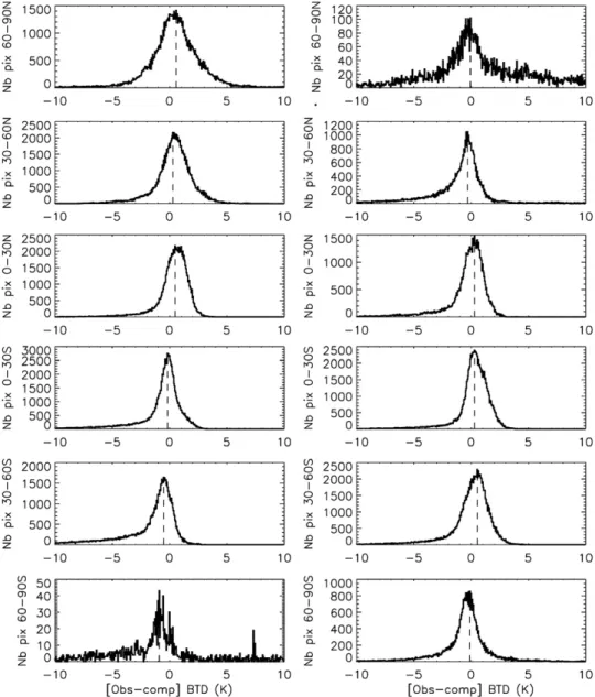
Figure 9 shows the frequency histograms of the dif-ferences at 12.05 mm between the observed and com-puted brightness temperatures (noted BTDoc) over ocean for all pixels identified as ‘‘clear sky’’ in the scene classification. The histograms are built from the daytime half orbits of July 2010 (left panel) and January 2011 (right panel) for 308-wide bands of latitude. The largest number of pixels is obtained in the Southern Hemisphere
FIG. 9. Frequency histograms of the difference between clear-sky observed and computed brightness temperatures over ocean on (left) July 2010 and (right) January 2011 during daytime. Each row from top to bottom corresponds to a 308 latitude band from north to south for channel 12.05 mm.
in the tropics and at midlatitude because of the ocean cover. The statistics are poor at 608–908S in July and 608– 908N in January because of prevailing nighttime condi-tions. For each distribution shown in Fig. 9, Table 4 gives BTDoc at the peak (BTDocp) and the percentage of
points within 61, 62, and 63 K from the peak. BTDocp
is found smaller than 0.5 K between 608N and 608S and smaller than 1 K globally, in absolute value. BTDoc is positive in the Northern Hemisphere in July and 0.3– 0.7 K smaller in January, whereas it is negative in the Southern Hemisphere in July and 0.6–1 K larger in Jan-uary. Moreover, the distributions show a tail toward negative values (down to 210 K) in the winter season of each hemisphere, especially at midlatitude. These results can be explained by the residual errors linked to the surface temperature and water vapor profiles in the simulations. The negative tail could be partly due to undetected dense layers at the surface. Table 4 shows that
typically 60% of the points are within BTDocp61 K
between 608S and 608N and 80%–96% of the points are within BTDocp 63 K (mostly dark polar regions
ex-cluded). The results obtained over land are reported in Table 5, showing significant biases of several kelvins mainly due to the uncertainty in the surface emissivity inferred from the IGBP/NSIDC surface type available on a 109 grid. The bias of 8–9 K in the northern tropics (08– 308N) is due to desert areas where clear-sky conditions are common. A large dispersion is observed with only 40%–60% of the points within BTDocp65 K.
2) OPAQUE LAYER
When the semitransparent cirrus cloud is above a low opaque layer, the background reference is computed using the FASRAD model whenever no suitable neighboring pixels are found. In this case, the model computes the cloud opaque radiance, that is, the blackbody radiance as
TABLE4. Differences between observed and computed brightness temperatures at the peak of each distribution shown in Fig. 9 over ocean (BTDocp) and percentage of points at 61, 62, and 63 K from the peak.
BTDocp(K) % at peak 6 1 K % at peak 6 2 K % at peak 6 3 K
July 2010 608–908N 0.6 45 72 86 308–608N 0.3 58 82 92 08–308N 0.5 70 91 96 08–308S 20.2 66 83 90 308–608S 20.5 58 74 80 608–908S 20.9 40 54 62 January 2011 608–908N 20.1 32 48 59 308–608N 20.3 54 72 80 08–308N 0.3 66 86 91 08–308S 0.3 69 90 95 308–608S 0.5 60 84 90 608–908S 20.1 60 78 86
TABLE5. As in Table 4 but over land and percentage of points at 61, 63, and 65 K from the peak.
BTDocp(K) % at peak 6 1 K % at peak 6 3 K % at peak 6 5 K
July 2010 608–908N 20.1 32 49 60 308–608N 0.9 17 30 43 08–308N 8.8 18 34 48 08–308S 1.7 21 38 52 308–608S 0.2 24 44 60 608–908S 1.6 17 32 47 January 2011 608–908N 3.1 14 28 41 308–608N 0.57 19 35 50 08–308N 7.9 23 43 57 08–308S 2.7 15 28 40 308–608S 4.6 15 28 40 608–908S 3.8 26 48 64
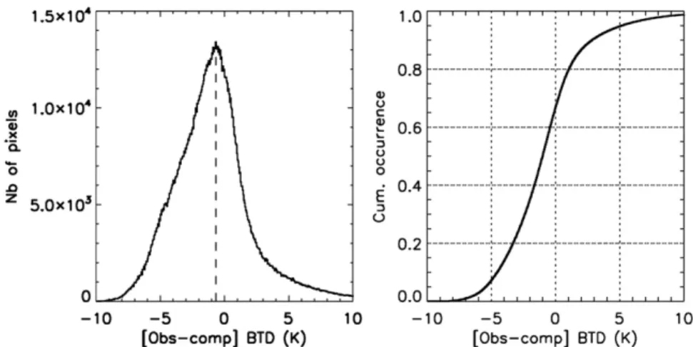
described in section 3. Figure 10 shows the frequency distribution (left) and cumulative occurrence (right) of the temperature difference between the observed and com-puted blackbody brightness temperature at 12.05 mm for low opaque clouds (type 20) in January 2011, over ocean between 608S and 608N. The distributions are built at the 1-km IIR pixel resolution using the centroid altitude and temperature inferred from the 5-km scene classification. The possible variability of the centroid altitude at 1-km resolution within each 5-km segment contributes to the width of the distribution, which peaks at 21 K with 80% of the pixels within 64 K. We found that positive differences prevail at low temperatures, below 240 K, which is similar to the observations made for the high-altitude opaque
clouds discussed before. The most negative differences are found for the denser warm clouds exhibiting differences of only a few hundred of meters between the top and centroid altitudes. A possible explanation for this negative bias is a temperature inversion at the top of the cloud not re-produced in the GEOS 5.2.0 model and leading to a posi-tively biased centroid temperature.
e. Overall effective emissivity and optical depth error estimate
For each channel, the overall effective emissivity un-certainty d«eff
k is derived from the three independent
contributions listed above assumed uncorrelated to maximize the error, so that
d«eff k 5[Rk BG 2Bk(T, Zc)]21f[(›Rk/›T)dTm]21(1 2 «eff k )2[(›Rk BG /›T)dTBG]2 1 «2eff k[(›Bk(T, Zc)/›T)dTBB] 2g1/2. (6)
Figure 11 shows the overall error estimate at 12.05 mm versus the difference between the background and the cloud thermodynamic temperature (y axis). Three values of effective emissivity are considered: 0.1 (left panel), 0.5 (center panel), and 0.9 (right panel). Back-ground (BG) brightness temperature errors of 1, 3, and 5 K are considered to represent the conditions expected over ocean (1, 3 K), for good cases over land (5 K) and for low opaque clouds (3, 5 K). The blackbody bright-ness temperature error is 1 K (Fig. 11a) or 3 K (Fig. 11b) for the highest emissivity (0.9). The error on the back-ground brightness temperature is the prevailing source of uncertainty for low emissivity retrievals. For elevated clouds allowing a BG minus blackbody temperature
difference greater than 50 K, the uncertainty associated with an effective emissivity of 0.1 is about 0.02 in the best conditions (1-K BG error), slightly degrading to a mean value of 0.05 (0.1) for an error of 3 K (5 K). The error on the blackbody brightness temperature is the prevailing source of uncertainty for high emissivity retrievals (right panel) with no significant impact from the BG temperature. The uncertainty is smaller than 0.05 for elevated clouds (BG minus blackbody tem-perature smaller than 50 K) and remains smaller than 0.1 for a BG minus blackbody temperature difference of 25 K.
The statistical error on the effective optical depth is derived from Eq. (4) and d«effat 12.05 mm as follows:
FIG. 10. (left) Frequency distribution and (right) cumulative occurrence of the difference between observed and computed blackbody brightness temperatures for low opaque clouds (type 20) in January 2011, over the ocean between 608S and 608N for channel 12.05 mm.
dODeff 5d«eff/(1 2 «eff). (7)
Figure 12 shows the overall effective optical depth relative error derived from Eq. (7) using the same pre-sentation as in Fig. 11, with the effective emissivities of 0.1, 0.5, and 0.9 corresponding to effective optical depths of 0.1, 0.7, and 2.3, respectively. Similar relative errors are found for optical depths of 0.7 and 2.3, of 5%– 20%. Small effective optical depths of 0.1 can be re-trieved with an error of 20%–50% for BG errors of 1 K or even 3 K in case of very cold clouds overlying a warm surface as found in tropical areas. The error is between 5% and 20% in case of large effective optical depths (2.3) for blackbody errors of 1 K (3 K) when the BG minus blackbody temperature remains greater than 20 K (45 K).
7. Results and discussion
As discussed in section 5, the visible optical depth can be related to the effective optical depth at 12.05 mm inferred from the effective emissivity with an estimated
2.25 ratio in the tropics for ice crystal diameter larger than 45 mm. Figure 13 shows the distributions of the IIR cloud optical depth at 12.05 mm (IIR OD) defined as 2.25 3 ODeff(top row), and associated uncertainties
(bottom row) between 308N and 308S, at the IIR pixel resolution and for 50 consecutive orbits in January 2011. The results are shown for scenes composed of one high STC only (no aerosols) (left, scene 21) and one high opaque cloud (right, scene 40). The uncertainties are computed from Eqs. (6) and (7) for several back-ground and blackbody brightness temperature errors chosen to represent the expected conditions based on the sensitivity analysis presented in section 6. They are plotted for background brightness temperature errors equal to 1, 3, and 5 K for semitransparent clouds (type 21) and 1 K for opaque clouds (type 40). Black-body brightness temperature errors are 1 K for semi-transparent clouds and 1 or 3 K for opaque clouds. Negative effective emissivities, which result in no op-tical depth retrievals, are found in typically 8% (20%) of the 21 cases over ocean (over land) because of re-trieved background temperatures larger than the ob-servations [cf. Eq. (1)]. This qualitatively confirms the
FIG. 11. Overall effective emissivity error vs the difference between the background and the blackbody brightness temperatures (y axis) for effective emissivities 5 (left) 0.1, (middle) 0.5, and (right) 0.9. Background brightness temperature errors are 1 K (red), 3 K (green), and 5 K (black). Blackbody brightness temperature errors are (a) 1 K or (b) 3 K. Channel is 12.05 mm.
larger background uncertainties above land than above ocean. Opaque clouds (type 40) have a large range of optical depths. Here, the optical depth is not retrieved in typically 10% of the cases due to blackbody tem-peratures found lower than the observations leading to effective emissivity values greater than 1. The distri-bution peaks at total optical depths between 4 and 6. For optical depths greater than 6.7, or effective emis-sivities greater than 0.95, the results are very sensitive to the blackbody brightness temperature used in the retrieval.
Figure 14 shows the 2D distribution of the IIR cloud optical depth at 12.05 mm and collocated optical depths retrieved by CALIOP in the visible channel (532 nm) in the tropics between 308S and 308N during January 2011 for all the scenes composed of a single high STC (types 21 1 30 1 31; Table 2) well observed by both instru-ments. We mix here CALIOP optical depths inferred from two different techniques, which use either a default or a retrieved lidar ratio (Liu et al. 2005). The latter is typically applied to nighttime data and optical depths greater than 0.3. The color code represents the decimal logarithm of the number of points found at 5 km resolution
in a given range of IIR and CALIOP optical depths. Black solid lines of slope 1 are superimposed for com-parison with the anticipated relationship in case of large ice crystals. The IIR dispersion at low optical depth is about 0.05–0.2 over sea and 0.1–0.2 over land, consistent with background brightness temperature errors of 1–5 K (see Figs. 12 and 13). A very good agreement is observed, with CALIOP to IIR median ratios of 0.8–1.1 over sea and 0.8–1 over land for optical depths greater than 0.05 and 0.1, respectively. Results also show a remarkable sensitivity of both instrument and method. Indeed, even for small optical depth retrievals, our method produces results very close to those retrieved with CALIOP, down to values of 0.05. The comparisons with CALIOP cirrus cloud optical depths constitute a successful validation of the IIR retrievals and uncertainty estimates. The disper-sions are quantitatively explained by the sources of errors in the IIR retrievals.
Figure 15 shows the frequency distribution of single high STC IIR optical depths over ocean and land. This distri-bution exhibits a nearly exponential shape with mean values respectively equal to 0.47 and 0.59. This difference, which appears to be due to more frequent very thin cloud
FIG. 12. Overall effective optical depth relative error vs the difference between the background and the blackbody brightness temperatures (y axis) for ODeff5(left) 0.1, (middle) 0.7, and (right) 2.3.
Back-ground brightness temperature errors are 1 K (red), 3 K (green), or 5 K (black). Blackbody brightness temperature errors are (a) 1 K or (b) 3 K. Channel is 12.05 mm.
layers over the ocean than over land, may not be signifi-cant because of the respective sources of uncertainty.
8. Conclusions
The IIR/CALIPSO algorithm for the retrieval of high-altitude cloud effective emissivity and optical depth in each IIR channel is designed around the ver-tically resolved information reported by CALIOP collocated observations, allowing one to build an IIR scene classification under the CALIOP track. The analysis focuses on cirrus clouds when they are found alone in the atmospheric column or when CALIOP identifies an opaque cloud underneath. The correction for the so-called background radiance that would be observed in the absence of the studied cloud is made from nearby observations or derived from the FASRAD model using GMAO GEO5 meteorological data and surface types from the IGBP–NSIDC products. The vertical layer structure reported by CALIOP is used to determine the layer(s) centroid altitude and temperature
inferred from the GMAO GEO5 model to compute the equivalent blackbody radiance at the top of the atmo-sphere using the FASRAD model. The analysis is per-formed for IIR pixels collocated with the CALIOP track and extended to the neighboring (within 50 km) IIR swath pixels for which the brightness temperature does not differ by more than 1 K in average for the 3 IIR channels. Effective IR optical depths are inferred from the effective emissivity retrieved in each IIR channel. They correspond roughly to half of the total optical depth depending on the atmospheric conditions and ice crystal sizes. A detailed sensitivity analysis is provided. The performances improve with the radiative contrast between the background scene and the studied cloud. The retrieval of low effective emissivity is mostly sen-sitive to the correction for the background radiances whereas the blackbody radiance is the prevailing source of uncertainty at high emissivity. The blackbody radi-ance is found in agreement with the observations for the denser clouds identified as opaque by CALIOP ex-hibiting a difference of 400 m between the top and
FIG. 13. (top) Distributions of IIR optical depth and (bottom) associated estimated un-certainties between 308N and 308S for 50 consecutive orbits (about 3 days) in January 2011 and for (left) scenes composed of one high STC only (scene 21) as compared with (right) one high opaque cloud (scene 40). Background brightness temperature errors are 1 K (red), 3 K (green), or 5 K (black) for scenes 21 and 1 K for opaque clouds (scene 40). Blackbody brightness temperature errors are 1 K for semitransparent clouds (scene 21) and 1 K (red) or 3 K (green) for scenes 40. Channel is 12.05 mm.
centroid altitudes. Background brightness tempera-tures are typically retrieved with a bias from 21 to 1 K over ocean varying with the latitude and the season with 60% of the retrieval within 61 K. Larger biases of several kelvins are observed over land because of er-rors on surface emissivities. In case of low opaque clouds, a negative bias of 21 K is observed with a dis-persion of 64 K.
Comparisons of collocated IIR and CALIOP opti-cal depths of high-altitude single-layer tropiopti-cal STCs for January 2011 show an excellent consistency with the theoretical analysis. Very good agreement is observed
on average with no significant bias detected. The sen-sitivity of the method is evidenced by the retrieval of very small cloud optical depths, very close to CALIOP ones, down to values of 0.05. Mean IR optical depths are 0.47 and 0.59 over ocean and over land, re-spectively. The dispersions at low optical depth are 0.05–0.2 over ocean, and 0.1–0.2 over land. Statistical analyses over the 5-yr CALIPSO database should al-low refining these values. Optical depths of 5 on aver-age are found for CALIOP elevated opaque clouds.
Further improvements will include the use of 1-km-resolution lidar scene identification and ancillary sur-face data. Similarly, a deeper analysis is required to understand and to reduce the differences between ob-servations and theoretical computations in case of opaque clouds by incorporating more information from CALIOP and from the WFC reflectance during day-time, which in turn will contribute to improve the swath algorithm.
Acknowledgments. The authors thank F. Parol, C. Stubenrauch, and S. Ackerman for fruitful discussions. They are deeply grateful to the ICARE data center in France and to the CALIPSO team at NASA Langley Research Center for their help with the technical de-velopment of the IIR level 2 algorithm. The products are processed at NASA/LaRC and are publicly available at NASA/LaRC (http://eosweb.larc.nasa.gov/PRODOCS/ calipso/table_calipso.html) and ICARE (http://www.icare. univ-lille1.fr/). We also thank the IIR instrument de-velopment team at CNES, SODERN (M.-C. Arnolfo, G. Corlay, and colleagues), LMD/IPSL (F. Sirou, A. Pellegrin, D. Sourgen, and colleagues), and F. Gabarrot.
FIG. 14. The 2D distribution of IIR (y axis) and CALIOP (x axis) cloud optical depths for single-layered high-altitude semitransparent clouds (types 21, 30, and 31) in January 2011 (night and day) between 308S and 308N over (left) sea and (right) land. The color scale rep-resents the decimal logarithm of the number of points.
FIG. 15. Frequency of occurrence of cloud optical depths derived from IIR retrievals over sea (solid line) and land (dotted line) corresponding to Fig. 14.
The authors are thankful to CNES and CNRS (Centre National de la Recherche Scientifique) for their support.
REFERENCES
Ackerman, S. A., W. L. Smith, J. D. Spinhirne, and H. E. Revercomb, 1990: The 27–28 October 1986 FIRE IFO cirrus case study: Spectral properties of cirrus clouds in the 8–12 mm window. Mon. Wea. Rev., 118, 2377–2388.
——, ——, A. D. Collard, X. L. Ma, H. E. Revercomb, and R. O. Knuteson, 1995: Cirrus cloud properties derived from High Spectral Resolution Infrared Spectrometry during FIRE II. Part II: Aircraft HIS results. J. Atmos. Sci., 52, 4246–4263.
Allen, J. R., 1971: Measurements of cloud emissivity in the 8–13 m waveband. J. Appl. Meteor., 10, 260–265.
Cooper, S. J., T. S. L’Ecuyer, and G. L. Stephens, 2003: The impact of explicit cloud boundary information on ice cloud micro-physical property retrievals from infrared radiances. J. Geo-phys. Res., 108, 4107, doi:10.1029/2002JD002611.
Dubuisson, P., V. Giraud, O. Chomette, H. Chepfer, and J. Pelon, 2005: Fast radiative transfer modeling for infrared imag-ing radiometry. J. Quant. Spectrosc. Radiat. Transfer, 95, 201–220.
——, ——, J. Pelon, B. Cadet, and P. Yang, 2008: Sensitivity of thermal infrared radiation at the top of the atmosphere and the surface to ice cloud microphysics. J. Appl. Meteor. Climatol., 47, 2545–2560.
Duda, D. P., J. D. Spinhirne, and W. D. Hart, 1998: Retrieval of contrail microphysical properties during SUCCESS by the split-window method. Geophys. Res. Lett., 25, 1149–1152. Fu, Q., and K. N. Liou, 1993: Parameterization of the radiative
properties of cirrus clouds. J. Atmos. Sci., 50, 2008–2025. Giraud, V., J. C. Buriez, Y. Fouquart, F. Parol, and G. Se`ze, 1997:
Large-scale analysis of cirrus clouds from AVHRR data: Assessment of both a microphysical index and the cloud-top temperature. J. Appl. Meteor., 36, 664–675.
Heidinger, A. K., M. J. Pavolonis, R. E. Holz, B. A. Baum, and S. Berthier, 2010: Using CALIPSO to explore the sensitivity to cirrus height in the infrared observations from NPOESS/ VIIRS and GOES-R/ABI. J. Geophys. Res., 115, D00H20, doi:10.1029/2009JD012152.
Holz, R. E., S. A. Ackerman, F. W. Nagle, R. Frey, S. Dutcher, R. E. Kuehn, M. A. Vaughan, and B. Baum, 2008: Global Moderate Resolution Imaging Spectroradiometer (MODIS) cloud detection and height evaluation using CALIOP. J. Geophys. Res., 113, D00A19, doi:10.1029/2008JD009837. Inoue, T., 1985: On the temperature and effective emissivity de-termination of semitransparent cirrus clouds by bi-spectral measurements in the 10-mm window region. J. Meteor. Soc. Japan, 63, 88–98.
Kahn, B. H., A. Eldering, M. Ghil, S. Bordoni, and S. A. Clough, 2004: Sensitivity analysis of cirrus cloud properties from high-resolution infrared spectra. Part I: Methodology and synthetic cirrus. J. Climate, 17, 4856–4870.
Kristja´nsson, J. E., J. M. Edwards, and D. L. Mitchell, 2000: Impact of a new scheme for optical properties of ice crystals on climates of two GCMs. J. Geophys. Res., 105 (D8), 10 063–10 079. Liu, Z., A. H. Omar, Y. Hu, M. A. Vaughan, and D. M. Winker, 2005:
CALIOP algorithm theoretical basis document. Part 3: Scene classification algorithms. PC-SCI-202 Part 3, 56 pp. [Available online at http://www-calipso.larc.nasa.gov/resources/pdfs/PC-SCI-202_Part3_v1.0.pdf.]
——, and Coauthors, 2008: Airborne dust distributions over the Tibetan Plateau and surrounding areas derived from the first year of CALIPSO lidar observations. Atmos. Chem. Phys., 8, 5045–5060.
——, and Coauthors, 2009: The CALIPSO lidar cloud and aerosol discrimination: Version 2 algorithm and initial assessment of performance. J. Atmos. Oceanic Technol., 26, 1198–1213. McClatchey, R. A., R. W. Fenn, J. E. A. Shelby, F. E. Voltz, and
J. S. Garing, 1972: Optical properties of the atmosphere. Research paper AFCRF-72-0497, 108 pp.
Mitchell, D. L., 2002: Effective diameter in radiation transfer: General definition, applications and limitations. J. Atmos. Sci., 59, 2330–2346.
——, A. Macke, and Y. Liu, 1996: Modeling cirrus clouds. Part II: Treatment of radiative properties. J. Atmos. Sci., 53, 2967– 2988.
Parol, F., J. C. Buriez, G. Brogniez, and Y. Fouquart, 1991: Information content of AVHRR channels 4 and 5 with respect to the effective radius of cirrus cloud particles. J. Appl. Me-teor., 30, 973–984.
Pavolonis, M. J., 2010: Advances in extracting cloud composition information from spaceborne infrared radiances—A robust alternative to brightness temperatures. Part I: Theory. J. Appl. Meteor. Climatol., 49, 1992–2012.
Platt, C. M. R., and D. J. Gambling, 1971: Emissivity of high layer clouds by combined lidar and radiometric techniques. Quart. J. Roy. Meteor. Soc., 97, 322–325.
——, S. A. Young, R. T. Austin, G. R. Patterson, D. L. Mitchell, and S. D. Miller, 2002: LIRAD observations of tropical cirrus clouds in MCTEX. Part I: Optical properties and detection of small particles in cold cirrus. J. Atmos. Sci., 59, 3145– 3162.
Ra¨del, G., C. J. Stubenrauch, R. Holz, and D. L. Mitchell, 2003: Retrieval of effective ice crystal size in the infrared: Sensitivity study and global measurements from TIROS-N Operational Vertical Sounder. J. Geophys. Res., 108, 4281, doi:10.1029/ 2002JD002801.
Sassen, K., and J. M. Comstock, 2001: A midlatitude cirrus cloud climatology from the Facility for Atmospheric Remote Sensing. Part III: Radiative properties. J. Atmos. Sci., 58, 2113–2127. Stephens, G. L., S.-C. Tsay, P. W. Stackhouse Jr., and P. J. Flatau,
1990: The relevance of the microphysical and radiative prop-erties of cirrus clouds to climate and climatic feedback. J. Atmos. Sci., 47, 1742–1754.
Stubenrauch, C. J., A. Che´din, G. Ra¨del, N. A. Scott, and S. Serrar, 2006: Cloud properties and their seasonal and diurnal vari-ability from TOVS Path-B. J. Climate, 19, 5531–5553. ——, S. Cros, A. Guignard, and N. Lamquin, 2010: A 6-year global
cloud climatology from the Atmospheric InfraRed Sounder AIRS and a statistical analysis in synergy with CALIPSO and CloudSat. Atmos. Chem. Phys., 10, 7197–7214.
Vaughan, M. A., D. M. Winker, and K. A. Powell, 2005: CALIOP algorithm theoretical basis document. Part 2: Feature de-tection and layer properties algorithms. Doc. PC-SCI-202, 87 pp. [Available online at http://www-calipso.larc.nasa.gov/ resources/pdfs/PC-SCI-202_Part2_rev1x01.pdf.]
——, and Coauthors, 2009: Fully automated detection of cloud and aerosol layers in the CALIPSO lidar measurements. J. Atmos. Oceanic Technol., 26, 2034–2050.
Wang, C., P. Yang, B. A. Baum, S. Platnick, A. K. Heidinger, Y.-X. Hu, and R. E. Holz, 2011: Retrieval of ice cloud optical thick-ness and effective particle size using a fast infrared radiative transfer model. J. Appl. Meteor. Climatol., 50, 2283–2297.
Wei, H., P. Yang, J. Li, B. A. Baum, H.-L. Huang, S. Platnick, Y. Hu, and L. Strow, 2004: Retrieval of semitransparent ice cloud optical thickness from Atmospheric Infrared Sounder (AIRS) measurements. IEEE Trans. Geosci. Remote Sens., 42, 2254– 2267.
Wilber, A. C., D. P. Kratz, and S. K. Gupta, 1999: Surface emissivity maps for use of satellite retrievals of longwave radiation. NASA Tech. Publ. TP-99-209362, 35 pp. [Available online at http://www-surf.larc.nasa.gov/cave/pdfs/Wilber.NASATchNote99.pdf.] Yang, P., K. N. Liou, K. Wyser, and D. Mitchell, 2000:
Parame-trization of the scattering and absorption properties of
individual ice crystals. J. Geophys. Res., 105 (D4), 4699– 4718.
——, H. Wei, H. L. Huang, B. A. Baum, Y. X. Hu, G. W. Kattawar, M. I. Mishchenko, and Q. Fu, 2005: Scattering and absorption property database for non-spherical ice particles in the near-through far-infrared spectral region. Appl. Opt., 44, 5512– 5523.
Yue, Q., K. N. Liou, S. C. Ou, B. H. Kahn, P. Yang, and G. G. Mace, 2007: Interpretation of AIRS data in thin cirrus atmo-spheres based on a fast radiative transfer model. J. Atmos. Sci., 64, 3827–3842.