A diagnostics architecture for component-based system engineering

A Diagnostics Architecture for Component-Based System Engineering by

Martin Ouimet

B.S.E., Mechanical and Aerospace Engineering (1998) Princeton University

Submitted to the Department of Aeronautics and Astronautics in Partial Fulfillment of the Requirements for the Degree of

Master of Science in Aeronautics and Astronautics at the

Massachusetts Institute of Technology June 2004

@

72 MASSACHUSETTS INS E OF TECHNOLOGY

JUL

12004

LIBRARIES

AERO

Department of Aeronautics and Astronautics May 14, 2004

2

Certified by ...

Charles P. Coleman Assistant Professor of Aeronautics and Astronautics Thesis Supervisor

Accepted by ...

dward M. Greitzer H.N. Slater Professor of Aeronautics and Astronautics

A Diagnostics Architecture for Component-Based System Engineering by

Martin Ouimet

Submitted to the Department of Aeronautics and Astronautics on May 14, 2004 in Partial Fulfillment of the

Requirements for the Degree of Master of Science in Aeronautics and Astronautics

Abstract

This work presents an approach to diagnosis to meet the challenging demands of modern engineering systems. The proposed approach is an architecture that is both hierarchical and hybrid. The hierarchical dimension of the proposed architecture serves to mitigate the complexity challenges of contemporary engineering systems. The hybrid facet of the architecture tackles the increasing heterogeneity of modern engineering systems. The architecture is presented and realized using a bus represen-tation where various modeling and diagnosis approaches can coexist. The proposed architecture is realized in a simulation environment, the Specification Toolkit and Requirements Methodology (SpecTRM). This research also provides important back-ground information concerning approaches to diagnosis. Approaches to diagnosis are presented, analyzed, and summarized according to their strengths and domains of applicability. Important characteristics that must be considered when developing a diagnostics infrastructure are also presented alongside design guidelines and design implications. Finally, the research presents important topics for further research.

Thesis Supervisor: Charles P. Coleman

Contents

1 INTRODUCTION

2 DIAGNOSIS AND FAULT-TOLERANCE 2.1 Diagnosis . . . . 2.2 Fault-Tolerance . . . . 2.3 Faults, Fault Types, and Fault Models 2.4 M odeling . . . . 2.5 Approaches to Diagnosis . . . . 2.5.1 Direct Observation . . . . 2.5.2 Probabilistic Inference . . . . . 2.5.3 Constraint Suspension . . . . . 2.5.4 Signal Processing . . . . 2.5.5 Discrete Event Systems . . . . . 2.6 Diagnosability . . . . 2.7 Other Considerations . . . . 2.8 Analysis and Summary . . . .

3 PROPOSED ARCHITECTURE

3.1 Hierarchical Architecture . . . . 3.2 Hybrid Architecture . . . . 3.3 Data Bus Architecture . . . .

4 ARCHITECTURE REALIZATION . . . . 15 . . . . 16 . . . . 18 . . . . 20 . . . . 2 1 . . . . 22 . . . . 23 . . . . 25 . . . . 27 . . . . 28 . . . . 3 1 . . . . 3 2 . . . . 3 3 36 . . . . 36 . . . . 39 -~~

~ ~

~

4.1 SpecTR M . . . . . 45

4.2 R ealization . . . . 46

4.2.1 Structure . . . . 47

4.2.2 Approaches . . . . 48

4.2.3 The Java API . . . . 53

4.3 Summary and Extensions . . . . 53

List of Figures

Generic System Representation . . . . Fault-Tolerant Controller Architecture . . . . A Simple AND Gate . . . . A Network of AND Gates and OR Gates . . . . . A Simple Automaton . . . .

Hierarchical Architecture . . . . Data Bus Architecture . . . . Agent Realization of the Conceptual Architecture

Diagnostics Architecture Structure . . . . Diagnosis using a Signal Processing Approach . . Diagnosis using Constraint Suspension . . . . Diagnosis using Discrete Event Systems . . . . 2-1 2-2 2-3 2-4 2-5 3-1 3-2 3-3 4-1 4-2 4-3 4-4 . . . . 14 . . . . 18 . . . . 23 . . . . 26 . . . . 29 37 41 42 48 49 50 52

List of Tables

2.1 Approaches to Diagnosis . . . . 34

Chapter 1

INTRODUCTION

Technological advances have pushed the boundary of what modern engineering sys-tems can accomplish. With the constant increases in computer performance, con-temporary engineering systems have come to rely heavily on automation for nominal operation. Automation has played a major role in meeting the performance and func-tionality demands expected of current engineering systems. However, these advances have also drastically increased the complexity of common modern systems. Ampli-fied complexity inevitably introduces an increase in the possible failures of advanced systems [13]. Even with enhanced quality control processes and other methods aimed at removing failures from systems, building systems without faults remains an elusive task. Given the assumption that faults are inevitably present in systems of moderate complexity, the need to find and correct these faults becomes an integral part of the performance of such systems. Consequently, modern engineering systems face the challenging task of diagnosing and accommodating unexpected faults. Furthermore, all systems should react to faults in a safe, non-destructive manner, so that the system can continue nominal operation or minimize operational losses.

Application domains where increasing dependence on automation and booming complexity can be observed include manufacturing, transportation, and space explo-ration [7,14,16,22,27,29]. Among these application domains, the need for reliability is extremely high, especially in safety-critical systems and mission-critical systems. Safety-critical systems are distinguished by potential physical harm to humans. Such

systems include aviation, manned space exploration, and nuclear power plant opera-tion. On the other hand, mission-critical systems may not involve potential physical harm to humans, but reliability in such systems is important because of the high cost of failure or the high cost of downtime. Such systems include unmanned space exploration, manufacturing systems, and power systems. The responsibilities put on safety-critical and mission-critical systems require that they be of utmost reliability or that, should they fail, they do so gracefully so as to minimize the cost of failure.

Evidently, as a system becomes more complex, diagnosing faults in such a system also becomes more difficult. Alongside increasing complexity, modern systems also display increasing heterogeneity [29]. This increase in heterogeneity introduces new challenges to system diagnosis and modeling. Continuous dynamics and discrete behavior need to coexist and new failure modes are introduced as a side effect of heterogeneity and complexity. The combination of disparate components into a single system introduces failure modes that cannot be isolated to single-component failures [13]. Not only do components need to be diagnosed at a low-level, but faults arising from interaction between components must also be captured. As a result, in order to meet the reliability targets, a reliable diagnostic infrastructure must be able to handle the complexity and heterogeneity of modern engineering systems.

A survey of the literature presents numerous diagnostic technologies [2,3,8,10,12, 17,24, 27, 29]. The proposed approaches display desirable diagnostic attributes for a breed of systems. Moreover, certain diagnostic technologies serve a special purpose very proficiently [19,27]. With the increasing heterogeneity of systems, a comprehen-sive diagnostics architecture should be flexible enough to combine various diagnostics technologies into the diagnostics strategy. Combining diagnostics approaches will enable the system designers to capitalize on the strengths of the various methods. Another interesting point to note is that the diagnostics strategy is very closely tied to the modeling of the system. In turn, the system model is dependent on the dynam-ics of the system. Consequently, as was previously elicited, realistically modeling the dynamics of modern systems will require some form of hybrid modeling to capture the full behavior of the system (even if it is to be approximated). As a result, the

diagnostics strategy will also need to incorporate hybrid capabilities.

This work presents a diagnostics architecture that is both hierarchical and hybrid. The hierarchical dimension of the architecture helps mitigate the complexity of mod-ern systems through levels of abstraction. By leveraging levels of abstraction, the responsibilities of the diagnosis component can be distributed. Moreover, the logic needed at the top level of the system can also be simplified to a more manageable level. Hierarchical diagnosis has been studied to a certain extent [6], but the concepts could be expanded further. Furthermore, hierarchical considerations have not been fully realized in a complete and flexible hybrid architecture. The concept of hierarchi-cal abstractions have been around for quite some time in a variety of fields (computer science, cognitive engineering, mechanical engineering, etc.). The benefits reaped by other fields can also carry over to the field of diagnostics.

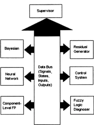
The hybrid dimension of the architecture enables the combination of diagnostics technologies into a comprehensive diagnostics framework. As Chapter 2 will reveal, there exists a plethora of approaches to diagnostics. While all of these approaches have the same goal - finding and accommodating faults in systems - the means by which they reach their goal can vary significantly. The hope is that a hierarchical and hybrid architecture can meet the diagnostics needs of increasingly complex and heterogeneous engineering systems. This work also presents a realization of the con-ceptual architecture using a data bus architecture and a simulation environment. The data bus architecture enables universal information dissemination and a plug-and-play environment for diagnostics technologies. Developing such a flexible framework will enable system designers to tailor their diagnostics strategy to the needs of their spe-cific project. Given the wide range of applications of this work, flexibility should be emphasized. The simulation environment presented enables system designers to test out their diagnostics strategy during the early phases of system design.

Creating a comprehensive diagnostic strategy for modern engineering systems is an important challenge. However, developing such a strategy from concept to produc-tion introduces another set of challenges. Not only is diagnosis development highly dependent on system development but diagnosis behavior is also difficult to verify

and validate. Given that many of the target systems for this technology (especially space exploration systems) operate in highly uncertain environments, validating and verifying the behavior of the diagnostics strategy becomes of utmost importance. While it would be impossible to predict all of the possible operating conditions of such systems, running a series of simulation provides a good starting point for veri-fying behavior. The reality of most diagnostics technologies is such that most faults need to be predicted in advance. While this reality unveils inherent limitations in the technology, a simulation environment can play an important role in estimating the performance of the system under novel faults.

Other development challenges include how to design systems that are diagnosable and how to understand how different system designs affect diagnosability. These challenges are not limited to this work only, but to any work on diagnostics. System decisions such as what sensors to include in a system affect not only the diagnostics infrastructure, but the system as a whole. However, if tradeoffs can be evaluated in an empirical manner (rather than through instinct or past experience), the decisions on system design and diagnosability implications can be fully understood. Other important challenges in system design (and not only in diagnostics design) is the idea of reuse. Reuse has often been cited as a viable means of reducing development cost and time to production. However, reuse faces multiple challenges that have led to rethink the benefits of reusing implementation. It has been argued that, perhaps, reuse has not been targeted at the right phase of the system lifecycle [28]. Design and specification may provide adequate phases of the lifecycle where reuse could be viable. Reuse of design and specification can potentially reduce cycle targets if applied

properly [28].

This work also presents an approach to system design [28] that attempts to capi-talize on design and specification reuse. The reuse methodology can also be applied to diagnostics design and specification. The proposed approach uses domain specificity and an executable design environment to enable specification reuse, verification, and validation. The environment provides a set of system engineering tools that enable system design and simulation in a component-based framework. In this framework,

components (in the form of design and specification) can be reused and combined into a complete system using a plug-and-play philosophy. Reuse can be more success-fully achieved within a specific domain (such as spacecraft design). Using a similar methodology, a set of diagnostics best practices for a specific domain can be devel-oped and tested during the system design phase. This methodology would ease the development cycle and provide a quantitative basis on which to evaluate diagnos-tics approaches. Furthermore, this methodology would enable the incorporation of diagnostics considerations incrementally into a system from the system's inception. Traditionally, diagnostics implications have been left to the end of the development cycle as an add-on feature. Delaying the considerations has the adverse effect that the diagnostics strategy will be limited to the design decisions made earlier in the system design.

In summary, this work provides a diagnostics strategy to tackle the increasing demands of modern engineering systems. Furthermore, this work provides a method-ology and an environment for tackling the challenges of developing and implementing the diagnostics strategy. This is accomplished through a proposed architecture that is both hierarchical and hybrid. Furthermore, the proposed architecture is realized and simulated in a component-based environment. This work does not address di-agnosability analysis, design iterations for didi-agnosability, problem size limitations (tractability), or diagnosis with humans in the loop. While those topics are all im-portant considerations, they fall outside the scope of this work. However, those topics are touched upon in relevant chapter and the reader is directed to appropriate sources for further insight.

This work is divided into 3 chapters, excluding the introduction (this chapter) and the conclusion. Chapter 2 provides an overview of the field of diagnosis, includ-ing descriptions of the various approaches that have been suggested in the literature. Chapter 2 also supplies background information, including definitions, problem sit-uation, and important considerations. Chapter 3 describes the proposed diagnostics architecture from a theoretical perspective. The theoretical perspective includes trea-tise on the hierarchical and hybrid nature of the architecture, as well as the conceptual

path into the architecture realization. Chapter 4 provides the physical realization of the architecture, with an emphasis on how this architecture can be realized in the proposed simulation environment. Finally, the conclusion (Chapter 5) provides clos-ing thoughts on the accomplished work, as well as suggestions for how this work can be further expanded.

Chapter 2

DIAGNOSIS AND

FAULT-TOLERANCE

Before embarking on a detailed discussion of diagnosis and relevant technologies, it is imperative to define the key terms. Perhaps the first question to answer should be What is Diagnosis?. The short answer to this question is diagnosis is the detection and explanation of malfunctions in a system. The term malfunction can be further refined to include any unexpected behavior of a system. However, to be able to define unexpected behavior, a model of expected behavior must be available and completely understood. Representing expected behavior of a system is the primary focus of modeling. tolerance is a concept very closely related to diagnosis. Fault-Tolerance represents the malfunction resolution to ensure that the system performs adequately. Not surprisingly, diagnosis and fault-tolerance go hand in hand because malfunction resolution can only occur once the malfunction has been detected and identified. Diagnosis and fault-tolerance form an important set of techniques and concepts that are relevant to many types of engineering systems.

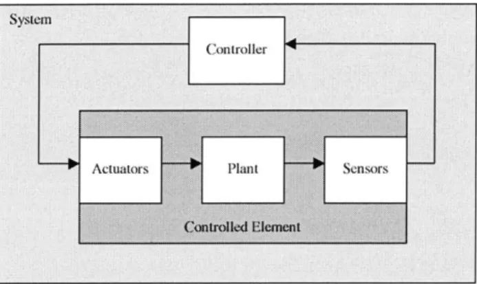
Before expanding on the preliminary definitions of diagnosis and fault-tolerance, other key terms need to be introduced. The Plant is generally understood to be the underlying controlled process. This process can be a vehicle (for example a spacecraft), a chemical process (for example a nuclear reactor), or any other physical process. The plant is usually fixed and contains natural dynamics that cannot easily

Figure 2-1: Generic System Representation

be changed (for example, an airplane is subject to certain aerodynamic forces that cannot be altered unless the airplane is redesigned). However, the goal of engineering systems is to get the plant to perform something specific and useful (for example, make an airplane fly from point a to point b). The way this is accomplished is by utilizing the plant dynamics in a way such that it meets the intended goals. The plant is typically equipped with a set of actuators that affect its dynamics. The component responsible for dictating what the plant should do and how it will do it is the controller. The controller utilizes the actuators to command the plant dynamics to achieve the desired goals. For example, in an airplane, the actuators include, among other components, the engines, the rudder, and the ailerons. Moreover, the controller needs a way to know the state of the plant's dynamics in order to issue the appropriate control commands. This is achieved via sensors that relay information about the various dynamics of the plant. For example, in an airplane, airspeed, angular rates, and altitude are common sensor measurements used to govern the control laws. The plant, the controller, and the set of actuators and sensors make up the System. A generic system architecture is depicted in Figure 2-1.

For a variety of reasons, the controlled element may not behave as the controller expects. Any deviation from expected nominal behavior of the controller is considered a fault. Faults can occur in actuators (for example, the aileron of an airplane not responding to commands), sensors (for example, the airspeed sensor returns corrupted data) or in the plant (for example, a power unit can go down). Regardless of where

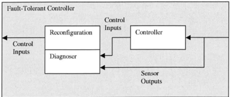
the fault occurs, the controller must be able to recognize the presence of off-nominal behavior and react appropriately. Therefore, a fault-tolerant controller should contain a diagnosis component as well as a fault-adaptation dimension (Figure 2-2. Although there are numerous available means to adapt to faults in the controlled element (for example robust controller design) [4], this work is concerned solely with a diagnosis approach supplemented with an adaptation mechanism.

2.1

Diagnosis

Diagnosis involves a multi-step process also sometimes called health-monitoring. Un-der nominal operation, the diagnoser remains a passive component of the system. However, the diagnoser must constantly analyze the behavior of the system to ensure that faults are detected in a timely manner. The diagnoser has 3 main responsibilities:

* Fault Detection

9 Fault Isolation

9 Fault Identification

Fault detection involves the realization that something wrong has occurred. Al-though this seems like a simple task, the diagnoser must be careful to discriminate between the occurrence of a fault and the occurrence of a disturbance. A Disturbance is a temporary unexpected shift in operating conditions (for example, a gust of wind). This distinction brings about interesting issues of sensitivity and false alarms. An ideal diagnoser would detect all faults and give no false alarms. In reality, however, increasing sensitivity will undoubtedly lead to false alarms. This topic is treated further in a subsequent section. Fault Isolation takes place after the detection that something has gone wrong. More specifically, fault isolation aims to attribute the fault to a specific component or set of components. Although faults can result as a sequence of failures in multiple components, this work focuses mostly on single fault diagnosis. Multiple faults are an important and challenging topic and are treated

briefly in a subsequent chapter. The final part of the diagnosis algorithm involves fault identification. Fault identification classifies the fault according to its observable behavior or a predefined fault model. The idea behind these 3 steps is to determine

what has occurred, where it has occurred, and what the implications are (what

correc-tive action may be taken, if any). Naturally, extracting this information is necessary to determine how the system can recover from the fault. Recovering from the fault is the responsibility of fault-tolerance.

2.2

Fault-Tolerance

There are a number of approaches to fault-tolerance. Traditionally, fault-tolerance has been implemented using physical redundancy. Physical redundancy involves du-plicating physical components so that when a component has been identified as faulty, the system can switch to a duplicated component and continue its function. However, given the increasing complexity of modern engineering systems, the number of com-ponents in a typical system is large and the duplication of every possible component is realistically not viable (sometimes for financial reasons, sometimes for physical re-strictions on allowed space and weight). However, for certain critical components, it is still common to use physical redundancy (power units are a good example). A different kind of redundancy, Analytical Redundancy, has gained popularity because it does not require the duplication of expensive components. Analytical redundancy uses redundancy in the functions of a system. For example, in the case of a two-engine aircraft, if one of the engine blows out and becomes non-functional, the aircraft can still function using the remaining engine. However, the thrust differential (between the blown engine and the functional engine) will impart a moment about the airplane's yaw axis. The corresponding yawing moment from the differential thrust vectors can be canceled out using the rudder. Additionally, functionality supplied using engine differential can be accomplished using the rudder. This type of redundancy and re-configuration can become quite complicated and must be considered carefully during the system design phase. Any type of closed-loop automated dynamics brings about

serious implications (especially in safety-critical systems) and should be analyzed and tested appropriately.

Another common form of failure-tolerance is the use of a "reset" or "recycle" command to cycle the faulty component out of its failed state. This type of failure-tolerance is common in computer systems (a reboot is often necessary after a computer has been on-line for quite some time). Analogously, this type of failure-tolerance is well-suited for components that accumulate data over time and can become saturated (like sensors). If a "reset" command is being issued to a given component, the entire system must be aware that the component is being recycled and hence is not avail-able until it is brought back on-line. Moreover, there is no guarantee that a given component will work correctly even after it has been "reset". It is entirely possible that the component could be malfunctioning because of causes other than state-based saturation. If this is the case, the component is identified as "broken" and another means must be sought to achieve fault-tolerance.

Finally, if the fault cannot be completely explained or if the fault is so severe that the system cannot adequately recover from it, it is often customary to resort to a "safe" mode of operation. This type of strategy is necessary for any critical system because it is impossible to guarantee the performance of the system in the face of every possible fault (or combination of faults). When in safe mode, the system is put in a state so that no critical actions can be taken that might endanger the system or the operators of the system. When a system is in safe mode, it requires outside assistance to resume operation or simply to decide on what to do next. For example, the spacecraft Deep Space One entered the safe mode when it had detected that it had lost its star tracker, a critical component vital to the normal operation of the spacecraft. Once safe mode was entered, mission operations entered on a long and complex rescue effort to salvage the spacecraft. Ideally, a controller should be able to react and adapt to any possible fault. However, in reality, it is usually not possible to adapt to every possible fault. It is customary to design a system to be able to handle a set of known failures. The safe mode is a popular way to handle failures that are not in the set of known faults.

Figure 2-2: Fault-Tolerant Controller Architecture

2.3

Faults, Fault Types, and Fault Models

A fault has been defined as a malfunction of a system. While this definition is accu-rate, the broadness of the definition makes it difficult to specify in great details what the possible faults of a system are. As mentioned in a preceding paragraph, in order to detect unexpected behavior, a model of expected behavior must be available. This model typically takes the form of a specification document, mathematical equations, or a plethora of other representations. Faults are then understood as observed be-havior that contradicts the expected bebe-havior as explained by the model. Faults can come in many flavors and must be further refined to enable deeper analysis.

Faults in a system can be divided into two main types -abrupt or discrete faults, and gradual or incipient faults. An example is in order to distinguish between these two different types of faults. Imagine a simple pipe/valve system. The valve regulates the flow of liquid through the pipe. If the valve is closed, no liquid flows. If the valve is open, liquid can flow. The first type of fault, abrupt or discrete fault, encompasses all faults that have a discrete set of states. If we consider the valve example and restrict the valve to a discrete set of states (OPEN or CLOSED), possible abrupt faults would be FAILED-OPEN and FAILEDCLOSED. These faults would reflect that the valve is expected to be open/closed (based on commands) but is in fact closed/open (the opposite state to the expected state). Since we assume that the valve cannot be in any other state when it fails, we can say that the valve is subject to two abrupt faults. The second type of fault, incipient or gradual fault, describes faults that degrade over time in a continuous fashion. Referring back to the valve example, if we suppose

that the valve can lose its stanching ability, we can describe an incipient fault. More specifically, when the valve is closed, we expect that no liquid passes through it. If after some operational amount of time, the valve starts eroding, a small amount of liquid can pass through it when it is in the closed position. Furthermore, the longer the valve is in operation, the more it erodes away and loses stanching ability. Gradually, the amount of liquid that can pass through gets larger and larger such that, eventually, the valve no longer serves its purpose. Typical incipient faults are not reversible and will only get worse as time elapses.

Faults can be further characterized based on how they manifest themselves in the system. Intermittent faults can be thought of in terms of the abrupt and incipient faults. When the two types of faults were presented, it was assumed that once the faults reveal themselves, the relevant component stays in the faulty state. Intermit-tent faults are different because they tend to reveal themselves periodically and to oscillate between faulty and nominal behavior. Referring to the valve example, for non-intermittent faults, if the valve enters the FAILEDCLOSED state, it will stay in that state unless some corrective action is taken. Similarly, if the valve has eroded enough that it is no longer useful, it will stay in a not useful (failed) state or get worse until corrective action is taken. However, intermittent faults describe faults that can appear and disappear. Referring back to the valve example, if the valve were to os-cillate between OPEN and CLOSED, the observed behavior would be an oscillation between OPEN and FAILED-CLOSED or between CLOSED and FAILEDOPEN depending on the expected behavior. These types of faults are especially difficult to diagnose because different samplings of the behavior yield different answers. Never-theless, these types of faults reveal themselves in regular patterns so that a careful analysis of the history of the system behavior can isolate the patterns and correctly diagnose the fault [19]. Another characterization of faults is that of transient faults. In certain systems, faults may occur at a specific time, but the fault does not produce anomalous behavior until much later after the fault has occurred. The time latency makes the diagnosis problem even more challenging since the location of the observed anomalous behavior is typically far removed from the occurrence of the fault.

Tran-sient faults are hard to detect until it is already too late and are even harder to isolate to individual components.

One of the main challenges of diagnosis and fault-tolerance is that faults are often novel. If one could predict the future and know what all the possible faults could be, the problem wouldn't be as complex and as interesting as it is. Unfortunately, the reality is such that one cannot predict the future. However, historical information and experience, especially in fields that have matured through a series of mishaps, can dictate what potential faults can be and how they can be remedied. It might be argued that if one knew what the faults will be, one can design the system in such a way that the fault will not occur. While this statement is partly true for certain faults, many of the possible faults cannot be easily erased through design. Especially for faults that result from a highly uncertain operating environments. Furthermore, it is also likely that faults are present because of system design and cannot be eradicated without completely redesigning the system. However, those faults remain important and must be accounted for. One way to identify certain faults is to have a predefined model of what the behavior of the system would be if the given fault were to occur. As a result, if the relevant behavior is observed, the fault is assumed to have occurred. The classification of such behavior is often called a fault model or fault signature. Often times, it is customary to link the fault model to a predefined solution, if pos-sible (in the form of a rule-based system). Care should be taken to ensure that the observed behavior can only result from the occurrence of the fault and not from some other combination of events. If the behavior is explainable in other ways, automated resolution of the problem could lead to more catastrophic behavior. Failures and fault models form the basis for many of the approaches to diagnosis and fault-tolerance.

2.4

Modeling

As mentioned in previous sections, diagnosis concerns itself with the detection and explanation of unexpected behavior of a system (faults). In order to perform this task, the diagnoser must have a model of what is considered nominal behavior. Often times,

the model takes an analytical form either as a logical model (for discrete dynamics) or as a mathematical equation (for continuous dynamics). The model exists as a redundant system to the actual physical system. The model is typically fed all of the inputs that are fed to the controlled element. The model then predicts the expected outputs. The predicted outputs are periodically compared with the measured outputs of the physical system (from sensor measurements) 2-2. If a discrepancy is observed between predicted and measured output, a failure is said to have occurred and the diagnoser will go through a series of steps (called an algorithm) to explain the fault. The details of these algorithms will be explained in the following section. However, it is important to note the importance of modeling and the importance of sensors. The variables measured by sensors are often termed the observables. The granularity of the model and the granularity of the observables will dictate what can be diagnosed and what cannot be diagnosed. This point must be emphasized early in the design stages because the choice of sensors greatly affects the diagnosability characteristics of the system. Furthermore, the model used by the diagnoser must also receive great care in how detailed the behavior of each component should be. These considerations are extremely important and will be treated in more depth in the Architecture Realization Chapter (Chapter 4).

2.5

Approaches to Diagnosis

The approaches to diagnosis all have the common task of detecting and explaining faults in a system. However, the means utilized to achieve this task differ greatly among the approaches to diagnosis. The differences often stem from the model used to represent the behavior of the system. The model will dictate what algorithms can be applied and how those algorithms will function. Given the heterogeneity of system dynamics, there is no single way to model a system. Consequently, most of the listed approaches have abilities to diagnose certain types of faults but no approach is positioned to encompass all types of faults. In order to adequately model typical modern engineering systems, existing approaches must be mixed and matched. The

listed approaches encompass the most relevant approaches for the context of this work. Other approaches are certainly possible. The presented list provides a feasible set that is in no way complete. For the sake of brevity, approaches not relevant to this work have been touched upon in the analysis section, but they have not been presented in details in this section. For further details about the listed approaches or other possible approaches, the reader should consult source [4].

2.5.1

Direct Observation

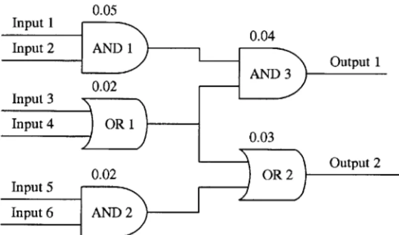
Perhaps the most basic form of diagnosis is that of direct observation. To explain direct observation, consider the AND gate in Figure 2-3. The behavior of the AND gate can be easily described using a truth table. Inputs and outputs can take any of two discrete values (1 or 0). If both inputs have a value of 1, the output will have a value of 1. Any other combination of inputs will yield an output value of 0. If sensors are available to measure the values of input 1, input 2, and the value of the output, the diagnosis can be performed directly. For example, if it is observed that input 1 and input 2 have a value of 1 but that the output has a value of 0, the diagnoser can automatically conclude that the AND gate is broken. Furthermore, it can be assumed that the AND gate is broken with its output being 0 regardless of the inputs (this preliminary conclusion can be later revised after more behavior is observed). The direct observation approach can include more details such as how long the output has had a value of 0 to reflect the potential latency in reaction to changing inputs. Direct observation represents the most reliable form of diagnosis and perhaps the most simple. Detecting and isolating failures is trivial in direct observation diagnosis, but the corrective action still needs to be carried out.

However, unfortunately, direct observation is typically not possible in practice because not all inputs and all outputs are measured by sensors. The complexity of most systems prevents this possibility. Since direct observation is usually not possible, the concept brings about the important topic of partial observability. In all complex systems, the state of the system is not completely observable and must be inferred based on the available information (sensor measurements). Often times the

Input 1

Output AND

Input 2

Figure 2-3: A Simple AND Gate

inference mechanism poses an important challenge because there typically isn't only one possible diagnosis given a set of observations. The challenge is to determine the most likely possible diagnosis (or system state) given the evidence and to take the appropriate action. However, acting on the inferred state should take into account that the inferred state might be erroneous. If further evidence becomes available and contradicts the previous inference, a new inference should be carried out. This type of functionality involves non-determenism and probabilistic analysis and is the subject of the following subsection.

2.5.2

Probabilistic Inference

Probabilistic Inference, sometimes called Bayesian Inference [1,11], refers to the pro-cess of reaching a conclusion based on a most likely criteria (highest probability of being right) given the available evidence (observations). This method contrasts with direct observation, which is completely deterministic. The term probabilistic covers the fact that probabilities are assigned to potential failures of components. As infor-mation becomes available through sensor measurements, the probabilities of failure of relevant components are updated. If unexpected behavior is observed, the com-ponent with the highest probability of failure is inferred to have failed. The initial probabilities of failure can be allocated based on historical data or test data although this type of information is not always available. Nevertheless, even though historical information might not be available, probabilities still need to be applied to failure events. The assignment of probabilities is a popular debate because it is often done subjectively [13]. Even though the assignment of probabilities may not be perfect, probabilistic inference remains one of the few approaches that provides a solution to the partial observability challenge.

The probabilistic inference approach is used for networked components that can-not be directly observed. Figure 2-4 represents a simplified network of components with partial observability. Although this example is somewhat of a toy problem, it nevertheless illustrates the ideas and applications behind the algorithm. The indi-vidual gates in the network can be construed as components within a system or as subcomponents within a component. The level of granularity selected by the system designer does not affect the functionality of the algorithm.

Returning to the example of Figure 2-4, the numbers assigned to each gate are assumed (or known) probabilities of failures. Even though some of the components appear to be identical, different probabilities are assigned to each component in order to augment the relevance of the example. The observables are the Inputs (numbered 1 through 6) and the Outputs (numbered 1 through 2). The values of the intermediate steps between Inputs and Outputs are not directly observable. However, a truth table for the network is available for the model of the system. Although the truth table is too long to print in its entirety, some important characteristics can be highlighted:

" If Input 1 or Input 2 (or both) is 0, Output 1 is 0 * If Input 3 and Input 4 are 0, Output 1 is 0

" Otherwise, Output 1 is 1

* If Input 5 and Input 6 are 1, Output 2 is 1

" If Input 3 or Input 4 (or both) is 1, Output 2 is 1

* Otherwise, Output 2 is 0

The model relationships having been established and the observables having been defined, different failure scenarios can be analyzed. For the first scenario, let's assume that Input 1, Input 2, and Input 3 have been observed to be 1. Additionally, Output 1 has been observed to be 0 and Output 2 has been observed to be 1. Given the logical relationship between the components, Output 1 should be 1. Consequently, a fault is inferred to have occurred. The algorithm should narrow down the candidates

for failures to AND 1, AND 3, and OR 1 (given the logical relationship). How the discrimination between the candidates occurs depends on the algorithm. A simple algorithm would pick the candidate with the highest probability of failure from the candidate set (in this case OR 1). A smarter algorithm would realize that since the Output 2 observable is consistent with the model, OR 1 must be functioning correctly (especially if it is observed that Input 5 or Input 6 is 0). If this is the case, OR 1 would be eliminated from the candidate set and a new potential candidate would be selected based on probability (in this case, it would be AND 3). This example is fairly simple. In more complex examples, more probabilities may need to be calculated based on the observables and the model. In all cases though, it is highly unlikely that the fault can be isolated to a single component without resorting to probability analysis for discrimination. Constraint suspension, the topic of the next section, takes a similar approach without the probability analysis.

The approach presented above represent an oversimplification of the probability concept known as Bayesian Inference. However, the ideas presented are similar to the basic concepts behind Bayesian Inference. The core idea is to treat observable values as random variables with probability distributions. The probability distributions (and consequently inferred probabilities) are updated as information becomes available. The original probabilities are typically called "a priori" probabilities and updated probabilities are typically called "a posteriori" probabilities. The process of updating probabilities is carried out using Bayes' theorem (where the term Bayesian Inference). For a more detailed treatise of Bayesian Inference and probability concepts, the reader is referred to [1, 11].

2.5.3

Constraint Suspension

Constraint suspension combines the benefits of direct observation and probabilistic inference while trying to avoid the drawbacks. Constraint suspension is best applied to logic systems or systems where the constraints of each component can be clearly identified and abstracted. The main idea behind constraint suspension is to iteratively suspend each component's constraints in the model (in the case of a logic system,

0.05

Figure 2-4: A Network of AND Gates and OR Gates

the truth table), and to verify if suspending a component's constraints renders the observables consistent with the model. If suspending a component's constraints causes consistency, that component is considered a failure candidate. Constraint suspension typically stops after generating the set of potential candidates. As in the case of probabilistic inference, it is possible that more than one candidate can explain the observed system behavior. How candidates are discriminated amongst each other is often left to further analysis. However, there can be a degree of suspicion based on how many rows in the truth table each suspension rules out. This process of discrimination is analogous to the discrimination process for probabilistic inference and is not guaranteed to be exact.

Referring back to the example problem depicted in figure 2-4, the algorithm can be illustrated. Iteratively suspending each component's constraints, the candidates for the faults remain AND 1, AND 3, and OR 1. Although the candidates are the same for both approaches, the conclusion is reached in a much more different fashion in each case. In the probabilistic case, candidates are ranked in terms of their probability of failure. In the constraint suspension case, candidates aren't ranked, but they are put into a set based on iteratively relaxing constraints. In the end, as is the case for many of the diagnostics problems, there is no unique answer to the diagnosis question and the best option left to the diagnostics infrastructure is to suggest a

most likely candidate. Further example could be drafted where probabilistic analysis and constraint suspension could yield different results (based on ranking), but the supplied example conveys the main ideas behind the approach. Both of the explained approaches work better on systems that can be modeled using discrete logic or systems that exhibit discrete dynamics. For systems modeled using continuous dynamics, a different approach must be considered.

2.5.4

Signal Processing

Although discrete logic can adequately model the dynamics of a wide range of systems, many systems also contain continuous dynamics. The most obvious type of continuous dynamics is a simple differential equation. The model of the system is thus fairly simple and the diagnostics task is also fairly simple granted that the necessary outputs can be readily measured. If the output of the system (in this case the dependent variable of the differential equation) can be observed, the continuous dynamics can be analyzed in some depth. Numerous approaches have been suggested for how to diagnose continuous signals [4]. However, most of these approaches consist of 2 similar steps:

" Residual Generation

" Residual Analysis and Decision-Making

The residual generation stage is analogous to the model/observation comparison stage of the probabilistic inference approach. More specifically, the measured signal is processed and subtracted from the predicted signal from the model. However, because the residual generation will compare a real-time signal with a model, sampling time comes into effect. Furthermore, noise considerations are important when processing continuous signals. A plethora of approaches dealing with noise and stochastic signals is available in the literature (Kalman Filter, Parity Space, etc.) [4]. However, for the scope of this work, the residual generation phase will be a simple comparison between measured output from the sensor and the model output. Noise considerations will be

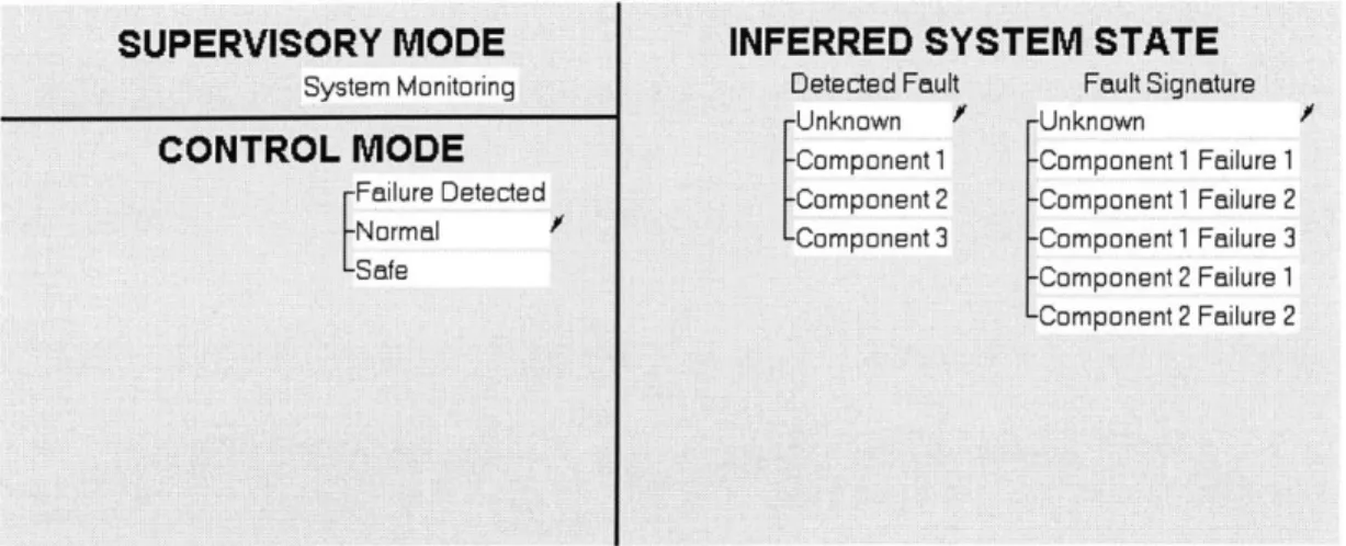
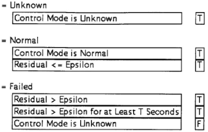
excluded. The second stage, analysis and decision-making deals with what action is to be taken given the residual's signature. Once again, this process can be very complex by incorporating continuous signals from various sensors and tracking the error (or integrals of the errors or derivatives of the errors over time). For the sake of this work, a simple approach is taken. A decision is reached by specifying an acceptable error band (typically denoted epsilon) and if the residual exceeds the error band, a fault is assumed to have occurred. Because signal processing and mathematical manipulations of signals go beyond the scope of this work, fault causes will be assigned directly to error bands that are too large. For example, for an airplane, giving an input to the rudder should enact a certain yaw moment. If the yaw moment measured by gyros and the yaw moment predicted by the model differ by too wide a margin, a failure in the rudder is assumed. The actual failure mode can be determined using fault models or can be assigned directly (for example, assume that the rudder is stuck in the neutral position if the measured response is very small). Diagnosis of continuous systems represents a very important branch of diagnosis and fault-tolerant control. Many of the systems targeted by the field of control engineering are systems modeled using differential equations. Consequently, a plethora of refined approaches are available in the literature [3,4,8]. However, with the increase use of computers to implement functionality, differential equations are not sufficient to describe the behavior of most systems. Discrete Event Systems provide a means to model systems to reflect the state-based dynamics of many contemporary systems.

2.5.5

Discrete Event Systems

To better understand Discrete Event Systems, some preliminary definitions should be given. A Discrete Event System (DES) is a discrete-state, event-driven system, that is, its state evolution depends entirely on the occurrence of asynchronous discrete events over time [5]. More specifically, discrete event systems are a way to model state-based systems that have well-defined transition rules between each state. Discrete event systems use automata as the basis for modeling. The automata can take on many of the traditional properties linked to automata (deterministic vs. stochastic, timed

FAIL

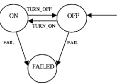
Figure 2-5: A Simple Automaton

vs. untimed, etc.). For the sake of this work, only finite-state deterministic automata will be considered. This limitation is not very restrictive because it corresponds adequately with the simulation platform that will be outlined in Chapter 4. Moreover, stochastic properties can be captured using the probabilistic inference described in a previous section. Also, non-determinism of an automaton can also be removed with a corresponding deterministic automaton [9]. For a brief review of automata theory, a simple automaton is presented in figure 2-5. The presented automaton has 3 states, (ON, OFF, FAILED), and can be cycled between each state using a set of 2 commands (TURNON, TURNOFF). The FAIL transitions (to the FAILED state) is triggered using a set of sensor readings and assumptions about what state the automaton should be in. Moreover, there can be more states depending on whether failure modes are available and the diagnoser needs to differentiate between each failure mode (might be necessary if reconfiguration is required).

The automaton has a start state, the OFF state. The automaton will be switched to the FAILED state only if it is detected that the automaton does not behave as it should (by the diagnoser component). Performing diagnosis on discrete event systems has been heavily explained in a number of sources [5, 12, 23,24]. The approach can be summarized as a series of 4 steps [23]:

1. Component Modeling

2. Component Composition

3. Creating a Sensor Map for the System

4. Revise Model Transitions to Reflect the Sensor Map

The first step involves the modeling of individual components. The second step, component composition, involves combining individual components into a single model automaton. The resultant model is a complete automaton that reflects the total be-havior of the system. The third step involves creating a sensor map using the set of available sensors of the system. The failure events of the system are modeled as states and sensor readings are defined for each state of the system. Transitions to failed states are achieved via unique combinations of sensor readings (from the global sensor map).

To better illustrate the discrete event systems approach, an example is given. Consider a simple pump/valve system (adapted from [23]). The pump and the valve are connected via a pipe. The pump causes fluid to flow through the pipe and the valve governs whether the fluid flows all the way through the pipe or if it stops at the valve. The pump has 4 states (ON, OFF, FAILEDON, FAILED-OFF) and the valve has 4 states (OPEN, CLOSED, FAILED-OPEN, FAILEDCLOSED). The system is also equipped with a sensor at the pump and a sensor at the valve (readings are HIGH or LOW depending on the presence of pressure at the sensor). If the pump in ON and the valve is OPEN, the pressure sensor at the valve should reads HIGH. Similarly, if the pump is OFF, the sensors at both the pump and the valve should read LOW regardless of the state of the valve.

A few failure scenarios can be considered. If the pump is assumed to be OFF and the valve is assumed to be OPEN (based on command history), but the sensor at the pump reads HIGH and the sensor at the valve reads LOW, it can be assumed that the pump has entered the FAILED-ON state and the valve has entered the FAILED-CLOSED state. Other similar failure scenarios can be considered. This example illustrates one of the main ideas behind this type of diagnosis. To perform this type of diagnosis successfully, unique failure signatures are necessary. For the presented failure scenario, if the sensor at the pump reads HIGH and the pump is assumed to be off, the assumed failure for the pump is FAILEDON. No other failure can cause this signature. To successfully model and diagnose systems using

discrete event systems, fault models must be known. But because this modeling approach uses a discrete set of states (including failure states), the diagnosable faults will be limited to the faults in the set of states. While this limitation might seem negative, discrete event systems nevertheless provide the basis for modeling many modern systems. Furthermore, they provide the ability to preform diagnosability analysis, a characteristic not easily achieved using the other approaches.

2.6

Diagnosability

Diagnosability is an important concept for the analysis and design of complex engi-neering systems. Diagnosability can be defined as the unique identification of failure events given available observations (sensor readings). In other words, diagnosability concerns itself with what can and cannot be diagnosed given a system design. Aside from the discrete event systems approach to diagnosis, the presented approaches to diagnosis do not directly address the notion of diagnosability. Probabilistic analysis cannot directly assert diagnosability because of the stochastic nature of the analysis. However, constraint suspension allows for diagnosability analysis if the fault signa-tures are known. Furthermore, constraint suspension can also enable a certain level of diagnosability analysis without fault models. For example, using iterative con-straint suspension, it is possible to determine whether the suspension of concon-straints of 2 components lead to the same set of constraints being discarded. If diagnosability analysis can be performed during the system design phase, useful design decisions can be made iteratively. A useful design platform would enable a system designer to determine diagnosability of a design and to understand diagnosability effects of adding/removing a sensor in the system. Moreover, a useful design platform would also enable a system designer to determine what faults would need to be diagnosed and to supply a set of sensors required to enable the correct diagnosis of the desired faults. Although diagnosability analysis is an important concept, such analysis will be treated only briefly in the context of this work.

2.7

Other Considerations

The given definitions capture the basic concepts behind diagnosis and fault-tolerance. Furthermore, the suggested approaches also provide a good overview of the techniques used to achieve the desired tasks. However, the information presented in this chapter still does not address all important considerations. First and foremost, most of the listed approaches have been presented only in the context of single failures. The theory of how to diagnose multiple failures is a very important topic. For some of the approaches (for example discrete event systems), diagnosing multiple failures comes more naturally than for other approaches (for example signal processing techniques). For other approaches, like probabilistic analysis, the possible combination of failures increases the required analysis and calculations considerably. Not only do conditional probabilities need to be calculated, but joint conditional probabilities must also be considered (including pairwise, triplewise, etc.). How to diagnose multiple failures remains an important and interesting topic although it falls outside the scope of this work.

Aside from multiple failures, trajectory tracking poses another interesting chal-lenge to the diagnosis task. Trajectory tracking involves keeping a time history of the system at hand so that the system state can be inferred using current information and past information about the system. Trajectory tracking is especially important for diagnosis approaches that rely on a most likely state inference approach (like Bayesian Inference). Since multiple states can be inferred at any one time, the non-determinism must be tracked over time. This way, when more information becomes available and the most likely state turns out to be erroneous, the next most likely state can be inferred using current and past information. How many trajectory to track and how much information to track is highly dependent on the system at hand. Nevertheless, trajectory tracking is an important characteristic of inference engines such as Livingstone [29].

Furthermore, this work and the corresponding diagnosis approaches refer to au-tomated diagnosis, that is, diagnosis carried out by a computer. However, for many

engineering systems, the automated diagnosis task is complemented with a human operator or supervisor. For most engineering systems, closed loop fault tolerance can be harmful, especially in the face of uncertainty. Typically, the automation will perform a preliminary diagnosis and further action (further analysis and problem resolution) is often left to the human component of the system. An example of di-agnosis with humans in the loop is when a system enters the safe mode after it has detected an unknown failure. Moreover, for novel faults and more complex faults that cannot be diagnosed using automation, the diagnosis task is often performed by the human supervisor. Other important considerations for system diagnostics in-clude human factors considerations, human-computer interaction considerations, and cognitive engineering considerations. The human dimension of diagnostics is an im-portant problem that has not received much attention. A comprehensive solution would incorporate the human operator as an integral component of the diagnostics infrastructure design. Some of the same concepts of automated diagnosis apply to diagnosis with humans in the loop (for example, diagnosability). However, the infor-mation needs to be presented to the human in a way conducive to readability and human analysis.

2.8

Analysis and Summary

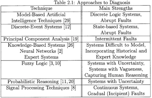
The presented list of approaches to diagnosis does not comprise a comprehensive inventory of available possibilities. Moreover, the approaches presented have been treated somewhat superficially for the sake of conciseness. The most important prop-erties have been exposed for the context of this work. For a more in-depth treatise of these approaches or for a more comprehensive list of approaches, sources [2,4, 5] provide a good starting point for further investigation. Nevertheless, the approaches presented represent an adequate set for the architecture presented in this work. The behavior of most engineering systems can be modeled using a mix of state machines (automata), equations, and truth tables. Consequently, incorporating discrete logic, state-based behavior, and continuous dynamics into the architecture will prove a

fea-Table 2.1: Approaches to Diagnosis

Technique Main Strengths

Model-Based Artificial Discrete Logic Systems, Intelligence Techniques [29] Abrupt Faults Discrete-Event Systems [12] State-based Systems,

Abrupt Faults Principal Component Analysis [19] Intermittent Faults

Knowledge-Based Systems [26] Systems Difficult to Model, Neural Networks [2] Incorporating Historical and

Expert Systems Expert Knowledge

Fuzzy Logic [3,10] Systems with Uncertainty, Systems with Vagueness, Capturing Human Reasoning Probabilistic Reasoning [11,20] Systems with Uncertainty Signal Processing Techniques [8] Continuous Systems,

Gradual (Incipient) Faults

sible modeling and diagnosis basis. Some of the approaches not covered in this work include approaches based on Fuzzy Logic, Statistical approaches (Principal Compo-nent Analysis being the most widely known), Knowledge-Based Systems, and Neural Networks. Table 2.1 provides a summary of the surveyed approaches, including their strengths and what types of faults they are most well-suited to diagnose. Moreover, since modeling is a big part of the problem, the strengths also include the types of systems typically targeted by the approaches.

It must be reemphasized that this table does not represent all of the possible approaches to diagnosis and modeling. However, these approaches were extracted from a recent survey of the literature on diagnosis. Now that a strong basis has been established on diagnosis and fault-tolerance, the architecture to include these approaches can be drafted. It must also be reemphasized that the listed approaches is not intended to represent the best approaches to diagnosis. As the summary ta-ble illustrates, all of these approaches have their redeeming values and the choice of approach is often a matter of expertise and preference. The purpose of this work is to provide a framework that is comprehensive yet flexible so that approaches can be mixed-and-matched at will depending on expertise and preference. It is also impor-tant to repeat that diagnostics is an imporimpor-tant consideration in any system but that

the level of sophistication is also highly dependent on expertise and mission needs. Many systems contain a very rudimentary set of diagnostics capabilities and it serves the purpose very well. Other systems, however, require more detailed diagnostics capabilities and the diagnoser can become quite convoluted. Whatever the project requirements, the hope is that the proposed architecture can meet the requirements of most diagnostics projects. Chapter 3 details the proposed architecture in more details.

Chapter 3

PROPOSED ARCHITECTURE

Chapter 2 covered the basics of diagnosis and fault-tolerance. Furthermore, Chapter 2 provided a survey of approaches to diagnosis and summarized the strengths of the proposed approaches alongside important considerations for system design. This chapter will describe the proposed diagnostics architecture for the component-based framework. The proposed architecture contains 2 main characteristics - a hierarchical decomposition to ease some of the complexity, and a hybrid dimension to enable the combination of multiple of the proposed approaches. Furthermore, this chapter also drafts the conceptual architecture's topology in the form of a data bus architecture. The data bus architecture will prove adequate for the realization in the simulation environment. In summary, this chapter provides the conceptual architecture that will form the basis for the architecture realization, presented in Chapter 4.

3.1

Hierarchical Architecture

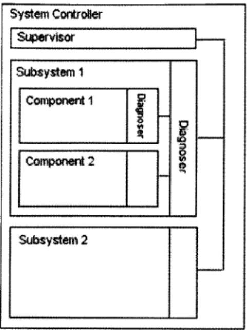
The proposed architecture uses an approach to system decomposition based on three levels, as outlined in [15, 28]. The system is first decomposed into subsystems and furthermore into components. The three levels can then be identified as system-level,

subsystem-level, and component-level [15]. This system decomposition is typical of

spacecraft systems and other large engineering systems. The diagnostics strategy performs tasks at each of these levels to obtain a complete picture of the state of the