HAL Id: insu-01820379
https://hal-insu.archives-ouvertes.fr/insu-01820379
Submitted on 12 Nov 2020
HAL is a multi-disciplinary open access
archive for the deposit and dissemination of
sci-entific research documents, whether they are
pub-lished or not. The documents may come from
teaching and research institutions in France or
abroad, or from public or private research centers.
L’archive ouverte pluridisciplinaire HAL, est
destinée au dépôt et à la diffusion de documents
scientifiques de niveau recherche, publiés ou non,
émanant des établissements d’enseignement et de
recherche français ou étrangers, des laboratoires
publics ou privés.
SPICAM/MEx data
Francisco Gonzalez-Galindo, Jean-Yves Chaufray, Francois Forget, Maya
García-Comas, Franck Montmessin, S.K. Jain, Arnaud Stiepen
To cite this version:
Francisco Gonzalez-Galindo, Jean-Yves Chaufray, Francois Forget, Maya García-Comas, Franck
Montmessin, et al.. UV dayglow variability on Mars: simulation with a Global Climate Model and
comparison with SPICAM/MEx data. Journal of Geophysical Research. Planets, Wiley-Blackwell,
2018, 123 (7), pp.1934-1952. �10.1029/2018JE005556�. �insu-01820379�
UV Dayglow Variability on Mars: Simulation With a Global
Climate Model and Comparison With SPICAM/MEx Data
F. González-Galindo1 , J.-Y. Chaufray2 , F. Forget3, M. García-Comas1 , F. Montmessin2 ,
S. K. Jain4 , and A. Stiepen5
1Instituto de Astrofísica de Andalucía-CSIC, Granada, Spain,2LATMOS, CNRS, Paris, France,3Laboratoire de Météorologie Dynamique, CNRS, Paris, France,4Laboratory for Atmospheric and Space Physics, University of Colorado Boulder, Boulder, CO, USA,5Space Sciences, Technologies and Astrophysics Research Institute, Université de Liège, Liège, Belgium
Abstract
A model able to simulate the CO Cameron bands and the CO+2UV doublet, two of the most
prominent UV emissions in the Martian dayside, has been incorporated into a Mars global climate model. The model self-consistently quantifies the effects of atmospheric variability on the simulated dayglow for the first time. Comparison of the modeled peak intensities with Mars Express (MEx) SPICAM (Spectroscopy for Investigation of Characteristics of the Atmosphere of Mars) observations confirms previous suggestions that electron impact cross sections on CO2and CO need to be reduced. The peak altitudes are well predicted
by the model, except for the period of MY28 characterized by the presence of a global dust storm. Global maps of the simulated emission systems have been produced, showing a seasonal variability of the peak intensities dominated by the eccentricity of the Martian orbit. A significant contribution of the CO electron impact excitation to the Cameron bands is found, with variability linked to that of the CO abundance. This is in disagreement with previous theoretical models, due to the larger CO abundance predicted by our model. In addition, the contribution of this process increases with altitude, indicating that care should be taken when trying to derive temperatures from the scale height of this emission. The analysis of the geographical variability of the predicted intensities reflects the predicted density variability. In particular, a longitudinal variability dominated by a wave-3 pattern is obtained both in the predicted density and in the predicted peak altitudes.
Plain Language Summary
The analysis of the radiation emitted by atmospheric species has long been used to derive information from planetary atmospheres. In this work we focus on two of the most intense emissions produced on the dayside of Mars in the UV range. For the first time we have simulated these emissions using a global model covering the whole planet, in contrast with all previous models that only considered a single vertical profile. We have validated our model with observations from the SPICAM instrument on board the European Space Agency spacecraft Mars Express. We have studied the variability of the emissions as predicted by our global model. We have found that the variability of the atmospheric density induces a similar variability in the emissions. While previous results indicated that both emission systems were produced basically from CO2only, we have found a significant contribution from CO toone of them. This complicates the derivation of the atmospheric temperature from the vertical variation of that emission.
1. Introduction
Since the beginning of the space era, remote sensing of UV atmospheric emissions has been one of the methods used to obtain information about the upper atmosphere of Mars (understood here as the upper mesosphere and thermosphere, that is, altitudes between around 80 and 180 km from the surface). UV atmo-spheric emissions arising from the Martian atmosphere were first detected by the Mariner 6, 7, and 9 missions (Barth et al., 1971, 1972; Stewart et al., 1972). These first measurements allowed identification of the main emission systems in the UV, including the CO Cameron bands, the CO Fourth Positive bands, the CO+
2 UV
doublet, the CO+
2 Fox-Duffendack-Barker system, and different emission lines arising from atomic Carbon,
atomic oxygen and atomic hydrogen. Analysis of Mariner data revealed that most of the emissions were ulti-mately produced by the effects of UV solar radiation and photoelectrons on CO2, the main constituent of the
Martian atmosphere (Barth et al., 1971). More recently, UV emissions have been observed by Spectroscopy
RESEARCH ARTICLE
10.1029/2018JE005556
Special Section:
Mars Aeronomy
Key Points:
• First global simulation of the UV dayglow on Mars
• An important contribution of CO to emission in the Cameron bands is found
• Comparison with SPICAM data suggests modifications in electron impact cross sections are required
Correspondence to: F. González-Galindo, [email protected]
Citation:
González-Galindo, F., Chaufray, J.-Y., Forget, F., García-Comas, M., Montmessin, F., Jain, S. K., & Stiepen, A. (2018). UV dayglow variability on Mars: Simulation with a global climate model and comparison with SPICAM/ MEx data. Journal of Geophysical
Research: Planets, 123, 1934–1952.
https://doi.org/10.1029/2018JE005556
Received 26 JAN 2018 Accepted 14 JUN 2018
Accepted article online 21 JUN 2018 Published online 31 JUL 2018
©2018. American Geophysical Union. All Rights Reserved.
for Investigation of Characteristics of the Atmosphere of Mars (SPICAM) on board Mars Express (MEx; Bertaux et al., 2005; Leblanc et al., 2006) and by Imaging Ultraviolet Spectrograph (IUVS) on board Mars Atmosphere and Volatile Evolution Mission (MAVEN; Jain et al., 2015; Stevens et al., 2015), adding N2 Vegard-Kaplan and Lyman-Birge-Hopfield bands to the list of identified emissions. Atmospheric temperature has been derived from the scale height of the UV doublet and the Cameron bands (Jain et al., 2015; Leblanc et al., 2006; Stiepen et al., 2015). NO𝛿 and 𝛾 bands have been identified as the dominant nighttime emissions (Bertaux et al., 2005; Gagné et al., 2013) on the basis of SPICAM observations and further analyzed later by IUVS (Stiepen et al., 2017).
The CO+
2UV doublet (≈ 289 nm) is produced by the de-excitation of the CO + 2(B
2Σ+) excited level to the (X2Π g) ground state. The main excitation mechanisms are photoionization and electron impact ionization of CO2.
CO2+ h𝜈 → CO+2(B
2Σ+) + e− (1)
CO2+ e−→ CO+2(B
2Σ+) + e−+ e− (2)
Fluorescent scattering of solar photons can also result in emission (Leblanc et al., 2006). While some estima-tions (Gronoff et al., 2012) consider this mechanism negligible, other works (Stiepen et al., 2015) have found it to be important above about 180 km. Given that we will focus on the altitudes around the emission peak, well below 180 km, we neglect here the excitation by fluorescent scattering.
The origin of the CO Cameron bands (≈ 180–260 nm) is the forbidden transition from the a3Π state of CO to
its ground state, X1Σ+. Excitation mechanisms are the photodissociation of CO
2, electron impact dissociation
of CO2, electron impact excitation of CO, and the dissociative recombination of CO+2:
CO2+ h𝜈 → CO(a3Π) + O (3)
CO2+ e−→ CO(a3Π) + O + e− (4)
CO + e−→ CO(a3Π) + e− (5)
CO+2+ e−→ CO(a3Π) + O1 (6)
In both cases, the radiative lifetime of the excited state is short, so collisional de-excitation is negligible in the upper atmosphere.
Different theoretical models have been developed in order to simulate the UV dayglow spectra and contribute to the interpretation of their measurements (Cox et al., 2010; Evans et al., 2015; Fox & Dalgarno, 1979; Gronoff et al., 2008; Jain & Bhardwaj, 2012; Shematovich et al., 2008; Simon et al., 2009). Whereas they use different approaches and techniques, they all coincide in that they are 1-D models, that is, they only consider variations with altitude. This allows for a detailed treatment of the different processes producing atmospheric emis-sion but decouples these models from the atmospheric variability produced by a variety of photochemical, physical, and transport processes. These 1-D models require as an input a background atmospheric structure (profiles of atmospheric density, temperature, and abundances of different species). Usually a handful of dif-ferent input profiles is used by these models to represent the seasonal/solar cycle variability. However, it is well known that the upper atmosphere of Mars is extremely variable (Bougher et al., 2017). The changing helio-centric distance of Mars and the seasonal evolution of the illumination conditions due the planetary obliquity produce a seasonal modification of the local heating terms in the upper atmosphere. The atmospheric cir-culation reacts to these modifications, inducing changes in the distribution of thermospheric species and, through adiabatic heating/cooling, modifying the radiation-driven temperature distribution (Bougher et al., 1999; González-Galindo et al., 2010). Temperature variations also affect the species distribution via modifica-tion of their scale heights, and the varying strength of the mixing produced by the general circulamodifica-tion can modify the altitude of the homopause (González-Galindo et al., 2009). The propagation of tides and other waves from the lower atmosphere induces additional variability in the thermospheric temperature, density and composition, as do the temporal variability of the solar output in the short (e.g., solar flares), medium (27-days solar rotation), or long (11-year solar cycle) terms. The presence of global dust storms in the lower
atmosphere can also induce significant modifications in the thermospheric thermal and wind structure (Bell et al., 2007; González-Galindo et al., 2015). Given the large variability induced by all these processes, it is clear that the generalization of some of the conclusions obtained from 1-D studies for all possible conditions is not guaranteed.
In this paper we describe the results of a Mars global climate model (GCM) that has been extended to incor-porate a dayglow model. In this way the effects of the atmospheric variability are reflected in the predicted emissions in a fully self-consistent way. The model is described in section 2. The outputs of the model are compared with MEx/SPICAM observations in section 3. In section 4 we will show, to our knowledge, the first global maps of the predicted CO+
2 UV doublet and the Cameron bands on Mars. The main conclusions are
summarized in section 5.
2. Methods
In order to simulate the Martian UV dayglow including the effects of atmospheric variability, we have extended the Mars GCM developed at the Laboratoire de Météorologie Dynamique (LMD-MGCM) with a module to calculate the intensities of the Cameron bands and the CO+
2UV doublet.
The LMD-MGCM is a ground-to-exosphere GCM for Mars. It is adapted from a terrestrial GCM by adding mod-els for processes relevant on the Martian atmosphere, such as the dust cycle, the water cycle, and the CO2
condensation-sublimation cycle (Forget et al., 1999). It was extended to the thermosphere and the iono-sphere by adding parameterizations of the physical processes important there (Angelats i Coll et al., 2005; González-Galindo et al., 2005, 2009, 2013). We use here the latest version of the model, including improve-ments such as the radiative effects of water ice clouds (Navarro et al., 2014), an improved parameterization of the 15μm cooling, and the day-to-day variability of the UV solar flux (González-Galindo et al., 2013, 2015). All the variability processes described in section 1 are included in the GCM.
The processes at the origin of the simulated emissions were described in equations (2) and (6). While the model already includes the calculation of photodissociation and photoionization rates, one key ingredient is missing to simulate the dayglow: the effects of the photoelectrons. So, the first step to simulate the dayglow with the LMD-MGCM was to include a model of the energy balance of the photoelectrons.
The energy of photoelectrons resulting from photoionization processes is calculated following Schunk and Nagy (2000):
Pe(E, z) = ∑ l ∑ s ns(z) ∫ 𝜆s 0 Iz(𝜆)𝜎s(𝜆)ps(𝜆, El)d𝜆 (7)
where Pe(E, z) is the photoelectron production rate for energy E and at altitude z (cm−3/s), n
s(z) is the abun-dance of the species s at altitude z (cm−3),𝜆
s is the ionization threshold for the species s (nm), Iz(𝜆) is the monochromatic solar flux at altitude z and wavelength𝜆 (s−1⋅ cm−2⋅ nm−1),𝜎
s(𝜆) is the monochromatic total photoionization cross section of the species s at wavelength𝜆 (cm2), and p
s(𝜆, El) is the branching ratio for the ion state with ionization energy El(adimensional). The energy E (eV) is calculated as E = E𝜆− El, with E𝜆 the energy of the photon with wavelength𝜆. An energy grid ranging from 0 to 200 eV with a step of 1 eV is implemented.
For this calculation, we consider the ionization of CO2, O2, O, N2and CO. The photoabsorption cross sections
are taken from Huestis et al. (2010) (CO2), Chan, Cooper, and Brion (1993) (CO), Kirby et al. (1979) (O2and
O) and Chan, Cooper, Sodhi, et al. (1993) (N2). The dissociation-ionization ratios and the branching ratios to
the different ionization channels are taken from Schunk and Nagy (2000). In addition, we consider 4 possible energetic levels for the CO+
2 ion, 9 energetic levels for O +
2, 5 for the O+ ion, 6 for N +
2, and 3 for CO+, with
branching ratios taken from Avakyan et al. (1999).
The degradation of the energy of the photoelectrons is calculated using the local approximation, in which the photoelectrons lose their energy in the same location where they are created. Comparisons of cal-culations using this approximation with more sophisticated electron transport models have shown good agreement in the altitude region where UV dayglow emissions are produced (Jain & Bhardwaj, 2011; Simon et al., 2009). Given the computation time constrains associated with the use of a GCM, we have chosen to calculate the energy degradation of the photoelectrons using the Analytical Yield Scheme (AYS) technique
(e.g., Bhardwaj & Jain, 2009). This technique provides a fast expression based on rigorous Monte Carlo calcu-lations, producing a good compromise between accuracy and calculation speed, ideal for implementation in a GCM. In particular, the photoelectron energy flux at the altitude layer Z and energy E is calculated from the photoelectron production rate using expression (4) in Jain and Bhardwaj (2011):
𝜙(Z, E) = ∫W200L
Pe(E, Z)U(E, E0) ∑
lnl(Z)𝜎lT(E)
dE0 (8)
where𝜎lT(E) is the total inelastic cross section for gas l (cm2), nl(Z) is its density (cm−3), and U(E, E0) is the
AYS (eV−1). See more details about the significance of the AYS in Bhardwaj and Jain (2009), Jain and Bhardwaj
(2011, 2012), and Bhardwaj and Jain (2013). For the AYS of CO2we use a modified version of expression (5) in
Jain and Bhardwaj (2011), due to a mistake in the original text:
U(E, E0) = A1Eks+ A2 ( Ek∕𝜖1.5 ) +E0B0e −x∕B 1 (1 + ex)2 (9)
where the values of the parameters are the same as in Jain and Bhardwaj (2011). For other gases (CO, N2, O2,
O) we use the expression of the AYS and the parameter values given by Singhal et al. (1980). The final step is the calculation of the excitation of the CO+
2(B 2Σ+
u) and the CO(a
3Π) levels by different
processes, and the corresponding volume emission rates (VERs). The excitation of the CO+
2(B2Σ+u) level by pho-toionization uses the CO2photoionization coefficient calculated by the model and the branching ratio from Avakyan et al. (1999). The excitation of the CO+
2(B2Σ+u) level by electron impact ionization of CO2uses the
calculated photoelectron energy flux and the cross section from Itikawa (2002). We use 50% crossover from the CO+
2(B2Σ+u) to the CO +
2(A2Π+u) excited state, according to Fox and Dalgarno (1979). The excitation of the CO(a3Π) level by CO
2photodissociation is calculated from the CO2photoabsorption coefficient calculated
by the model and the branching ratio to the (a3Π) state, taken from Lawrence (1972). The excitation of the
CO(a3Π) level by electron impact dissociation of CO
2and by electron impact excitation of CO is obtained from
the calculated photoelectron energy flux and the cross sections from Bhardwaj & Jain (2009; an analytical fit to the cross sections measured by Erdman and Zipf (1983)) and Furlong and Newell (1996), respectively. How-ever, it has to be taken into account that there are significant uncertainties in the cross sections of excitation of the CO(a3Π) level by electron impact on CO
2and CO. Detailed discussions about these uncertainties and their
impact on simulated dayglow can be found in Simon et al. (2009), Jain and Bhardwaj (2012), and Bhardwaj and Jain (2013). In short, both theoretical and experimental reasons, as well as comparisons of the predicted dayglow with observational results, point to a reduction of a factor of about 2 to 3 in these cross sections (Bhardwaj & Jain, 2013; Simon et al., 2009). We will explore the sensitivity to a reduction of these values by a factor of 3. Finally, the excitation by dissociative recombination of CO+
2is calculated using an efficiency of 0.87
of CO production, of which 0.29 is for CO(a3Π) state (Jain & Bhardwaj, 2012).
With the dayglow model incorporated into the LMD-MGCM, we have simulated the behavior of the Martian atmosphere during a full Martian Year. Except for the comparison with SPICAM observations, obtained at a period of low solar activity, we use as an input a solar flux appropriate for solar average conditions (see González-Galindo et al. 2005, 2009). While the solar activity is held constant during the simulated year, the solar flux getting to Mars’ upper atmosphere is modified during the simulated year following the variability of the heliocentric distance. To explore the sensitivity to the 11-year solar cycle, we also run simulations fed by a solar flux appropriate for generic solar minimum and solar maximum conditions. Although the LMD-MGCM does include the possibility of using the observed daily variable solar flux as an input (González-Galindo et al., 2013, 2015), this is not yet possible for the dayglow model. The reason is that the parameterization used to include the day-to-day variability of the UV solar flux relies on a division of the UV spectral range into relatively wide subintervals (typical width of about 5 nm). However, in order to calculate the initial energy flux of the photoelectrons, a good spectral resolution of the solar flux is needed (we use a 0.1-nm resolution in the calcu-lations shown here). Different strategies are being currently studied in order to add the day-to-day variability of the UV solar flux in the calculation of the dayglow, without further increasing the CPU time consumption. For the dust load, we use the “climatology” dust scenario described in Montabone et al. (2015). The effects of the global dust storm of MY28 are simulated using the daily-varying dust distribution observed during that period, following again Montabone et al. (2015).
3. Comparison With SPICAM Observations
The SPICAM instrument is a dual UV-IR spectrometer on board the European Space Agency MEx spacecraft. A recent description of the instrument and its current status can be found in Montmessin et al. (2017). The UV channel of SPICAM (SPICAM-UV) covers the range between 120 and 300 nm, approximately, including thus the region of the Cameron bands and the UV doublet. SPICAM-UV was in operation between orbit insertion at the end of 2003 until the end of 2014, when the UV channel failed. However, in late 2011 a significant drop in the efficiency of the image intensifier led to a significant degradation of the data quality (Montmessin et al., 2017), and data obtained after 2011 are not used here. Thus, the SPICAM-UV data set used here covers about eight terrestrial years (corresponding to 4 Martian Years, MY27 to MY30). Previous analysis of the UV dayglow observed by SPICAM has been published (Cox et al., 2010; Leblanc et al., 2006; Simon et al., 2009). However, these analyses used a restricted subset of the SPICAM-UV data set, obtained during the first Martian Year of operation. The full SPICAM data set was analyzed in Stiepen et al. (2015), but only for the purpose of deriving temperature from the scale height of the emission. Here we analyze the full SPICAM data set focusing on the variability of the intensities.
Starting from the publicly available SPICAM L1A data (not calibrated, see description in Appendix of Montmessin et al., 2017), we have made a first selection of the data according to geometry (data obtained using grazing limb geometry and located at the dayside) and data quality (nonflagged data and good signal-to-noise) criteria. Then we calibrated the data using the procedure described in Leblanc et al. (2006), including also their procedure to eliminate the background noise produced by the scattered light entering the spectrograph. The spectra are then binned in altitude, with a bin size of 2 km. For each retained orbit, a visual inspection of the vertical variability of the obtained spectra allows disregarding those orbits affected by straylight contamination. From the initial list of around 250 orbits, the filtering reduced the final number of orbits to 121. The obtained spectra are then integrated between 180 and 265 nm to obtain the intensity in the Cameron bands and between 286 and 292 nm for the UV doublet. As in previous works, due to the over-lap with the CO fourth positive bands, an altitude-independent reduction of 15% is applied to the spectrally integrated intensity to obtain the intensity in the Cameron bands (Cox et al., 2010).
A comparison of the obtained spectra with previous analyses of the SPICAM data set (Cox et al., 2010; Leblanc et al., 2006) shows a fully similar spectral shape but slightly lower intensities in our analysis for the Cameron bands and a larger difference (around 30%) for the CO+
2 UV doublet (not shown). This is mainly due to the
use of a different detector efficient area. As explained in Montmessin et al. (2017), the calibration procedure of SPICAM-UV data was updated in 2013, which resulted in a new curve of the detector efficient area (see Figure 3 in Montmessin et al. (2017) for a comparison of the old detector efficient area and the new one). In our analysis we use the new efficient area, while previous analyses made use of the old curve. Given that the new efficient area is larger than the old one, this results in lower values of the intensity (e.g., equation A2 in Leblanc et al., 2006). We have checked that when using the old efficient area curve, the agreement between our results and previous analyses is quite good.
The distribution of the SPICAM-UV Cameron bands observations as a function of season and latitude, with dif-ferent colors indicating data obtained in different Martian Years, can be seen in Figure 1. As mentioned before, only the peak intensities and altitudes obtained during MY27 had been analyzed before. The addition of data obtained during MYs 28, 29, and 30 allows the seasonal and latitudinal coverage to be extended. However, even when including all the SPICAM data, the coverage is far from complete, with important gaps in particu-lar in the winter hemispheres during solstices and at most latitudes during equinoxes. It is also important to note that the period covered by observations corresponds to a long and deep minimum in solar activity (see, for example, Figure 1 in González-Galindo et al. (2015)).
In order to compare the predictions of the model with the observational results, the model outputs have been interpolated to the exact location (latitude and longitude) and time (Ls, local time) of each SPICAM observation. For the comparison we have used a simulation performed with a solar flux appropriate for solar minimum conditions. The obtained modeled emission profiles are then integrated along the line of sight. The intensity of the emission at the peak and the altitude of the peak are extracted and compared to the observations.
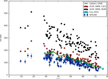
The comparison of the observed and modeled solar zenith angle (SZA) variability of the peak intensity of the Cameron bands is shown in Figure 2. The blue points represent the SPICAM observations, while the black
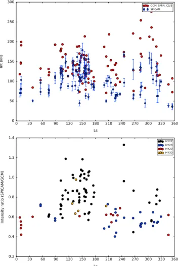
Figure 1. Seasonal and latitudinal distribution of the SPICAM-UV observations analyzed, with different colors indicating
data obtained in different Martian Years.
points are the model predictions for the simulation using the cross sections for excitation of the Cameron bands by electron impact on CO2and CO in Bhardwaj and Jain (2009) and Furlong and Newell (1996). In order to verify our analysis of SPICAM data, we have also added previous analyses of the SPICAM Cameron band data sets. In particular, the mean intensity shown in Figure 12 of Leblanc et al. (2006) and the data in Figure 6a of Cox et al. (2010) have been plotted as a green solid line and cyan points, respectively. Our analysis of SPICAM data yields lower intensities than those in previous works due to the use of the new detector efficient area. While both the observations and the model present a similar decrease of the peak intensity with increasing SZA, it can be clearly seen that the model strongly overestimates the emission, by a factor of about 3. As mentioned before, previous comparisons of 1-D model results with SPICAM measurements have found simi-lar overestimations of the modeled intensities, attributed to the uncertainties in the cross sections (Cox et al., 2010; Jain & Bhardwaj, 2012; Simon et al., 2009). The results of the model when reducing the cross sections for excitation of the Cameron bands by electron impact excitation on CO2and CO by a factor of 3 are shown by the
red points. A much better agreement with the observations is found, although there is still an overestimation of 25% on average. The cross section reduced by a factor of 3, producing better agreement with observations, is used in all the results that follow. Note also that the apparent increase of the intensity around SZA=20∘
Figure 2. Comparison of the peak intensity of the Cameron bands as a function of SZA. Blue points represent the
SPICAM measurements, black points the prediction of the model for the nominal simulation using solar minimum conditions, and the red points the model results for the simulation with reduced cross sections for excitation of the Cameron bands by electron impact. Previous analyses of the SPICAM data are shown with a green line (Leblanc et al., 2006) and cyan points (Cox et al., 2010). SZA = solar zenith angle. SPICAM = Spectroscopy for Investigation of Characteristics of the Atmosphere of Mars; GCM = global climate model; SZA = solar zenith angle.
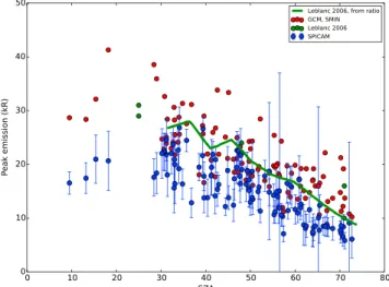
Figure 3. SZA variability of the CO+2UV doublet. Blue points represent our analysis of SPICAM data with vertical lines representing uncertainties. Green points are the peak intensities reported in Leblanc et al. (2006), while the green line is the UV doublet intensity variability obtained combining the variability of the Cameron bands intensities and the ratio between the UV doublet and Cameron bands intensities in Leblanc et al. (2006). Red points indicate the prediction of the model. SPICAM = Spectroscopy for Investigation of Characteristics of the Atmosphere of Mars; GCM = global climate model; SZA = solar zenith angle.
is an artifact of the uneven data distribution—the point closest to SZA=20∘ —and those around SZA=30∘ were obtained close to the perihelion season, where the emission has its annual maximum, as we will show later.
A similar plot, but for the CO+
2 UV doublet, is shown in Figure 3. No graph showing the SZA variability of
this emission was included in Leblanc et al. (2006) and Cox et al. (2010). We have nevertheless included UV doublet peak intensities for three ranges of SZA from Figure 8 of Leblanc et al. (2006), shown as green points in Figure 3. Leblanc et al. (2006) also studied the ratio between the emission in the UV doublet and in the Cameron bands as a function of altitude, finding a value of about 0.15 at 130 km. Analysis of IUVS/MAVEN data produced a similar value (0.14, Jain et al., 2015). So, we have multiplied the peak intensities in the Cameron bands extracted from Figure 12 of Leblanc et al. (2006) by 0.15, and the result is shown as the green line in Figure 3. As for the Cameron bands, the intensities we derive are slightly lower than those in Leblanc et al. (2006), again due to the use of the new detector efficient area. When using in our analysis the old efficient area curve, the obtained intensities are in quite good agreement with Leblanc et al. (2006). The comparison with the model shows a slight overestimation, of about 20% on average, when compared to our analysis of SPICAM results, of the order of the associated cross section uncertainties (Simon et al., 2009).
The seasonal variability of the peak intensity of the Cameron bands is shown in the top panel of Figure 4, both for SPICAM measurements (blue points) and for the model prediction when using the reduced cross sections (red points). The ratio SPICAM/GCM is plotted in the bottom panel, with different colors representing different Martian Years. It can be seen that the model predicts well the average intensity in the Ls =60–180∘ range, while overestimating the intensities during the rest of the year. The measured intensities do not show an increase from aphelion (Ls =71∘) to perihelion (Ls =251∘), while the model does. This may indicate that the model is overestimating the seasonal variability of the intensities and also a possible interannual variability not cap-tured by the model due to the use of a constant solar flux in the simulations. Most of the observations during the first part of the year, and in particular in the Ls =60–180∘ range, were taken during MY27, while many observations during the second half of the year were obtained during MY28 and most of the observations before Ls ≈ 45∘ correspond to MY29. As can be seen in Figure 1 of González-Galindo et al. (2015), the period from MY27 to MY29 corresponds to the declining phase of the solar cycle. That is, the solar flux was more intense during the first half of MY27 than during MY28 and MY29. This could explain the behavior displayed in Figure 4. A simulation using the observed day-to-day variability of the solar flux as in González-Galindo et al. (2015) would be needed to confirm this effect. As explained in section 2, this is not yet possible in the cur-rent version of the dayglow model, and diffecur-rent strategies are being studied to add this capability in a future version of the model.
Figure 4. (top) Comparison of the peak intensity of the Cameron bands as a function of season. Blue points represent
the SPICAM measurements, and the red points the model results for the simulation for solar minimum conditions with reduced cross sections for excitation of the Cameron bands by electron impact. (bottom) Ratio SPICAM/GCM. SPICAM = Spectroscopy for Investigation of Characteristics of the Atmosphere of Mars; GCM = global climate model.
We focus now on the comparison of the peak altitude for the Cameron bands, shown as a function of season in the top panel of Figure 5. In this case, the different colors represent data obtained in different Martian Years. Circles indicate SPICAM measurements, while squares represent the model predictions. The SPICAM-GCM peak altitude difference is plotted in the bottom panel of Figure 5. In general, good agreement is found, with both model and data clearly showing an increase in the peak altitude from aphelion to perihelion. Predicted peak altitudes are generally within 10 km of the measured values. Given that the peak altitude is linked to the atmospheric density, the good agreement between the SPICAM and the LMD-MGCM results indicates that the densities predicted by the model, and their seasonal variability, are correct to first order.
However, the model tends to overestimate the peak altitude around the aphelion season (Ls =45–90∘) and to underestimate it during the perihelion season. This is particularly true for data obtained during MY28, with an underestimation larger than 15 km. The perihelion season for MY28 was affected by the presence of a global dust storm. Previous modeling and observational results (Bell et al., 2007; González-Galindo et al., 2015; Withers & Pratt, 2013) have shown that the presence of dust storms in the lower atmosphere produces signif-icant effects on the upper atmosphere, among others an increase of the atmospheric density. As the altitude of the peak emission is intimately linked to the level of atmospheric density, an increase of the density due to a dust storm is expected to raise the altitude of the peak of the Cameron bands. As mentioned in section 2, the simulations described here use a climatological dust scenario, valid for years without a global dust storm. So, it is not surprising that the predicted peak altitudes are underestimated during the dust storm season of MY28. To check the effect of the global dust storm, we have made another simulation using the observed dust
Figure 5. (top) Comparison of the peak altitude of the Cameron bands as a function of season, with different colors
indicating data obtained in different Martian Years. Circles represent the SPICAM measurements, and squares represent the LMD-MGCM predicted altitudes for the climatological dust scenario. Blue inverted triangles represent the prediction of the model when using a realistic dust scenario for MY28. (bottom) SPICAM-GCM peak altitude difference, with different colors indicating different Martian Years. SPICAM = Spectroscopy for Investigation of Characteristics of the Atmosphere of Mars; GCM = global climate model.
latitudinal and seasonal distribution for MY28 following Montabone et al. (2015), including thus the global dust storm. The predicted peak altitudes are shown in Figure 5 as blue inverted triangles. An increase in the predicted peak altitudes of about 5 to 10 km is found with respect to the nominal simulation. This reduces the differences with the observational results at that season, but an underestimation of about 10 km is still present. This may indicate that the effect of the global dust storm on the thermospheric densities is underesti-mated by the model or that the seasonal variability of the peak altitude (i.e., the seasonal inflation/contraction of the atmosphere) is underestimated by the model.
4. UV Dayglow Global Maps
We focus here on the variability of the dayglow produced by the model at different geographical and temporal scales. As mentioned in section 3, we use in these simulations a reduction by a factor of 3 in the excitation cross sections of the CO(a3Π) level by electron impact on CO
2and CO, which yield better agreement with SPICAM
observations. As we are interested now in the variability of the emission, and not on the absolute values, the results shown below use a solar flux appropriate for solar average conditions.
4.1. Seasonal and Latitudinal Variability at the Emission Peak
We focus first on the seasonal and latitudinal variability of the peak magnitudes (intensity at the peak and altitude of the peak) for the two simulated emission systems. To mimic the observations of these emissions,
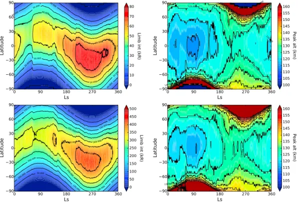
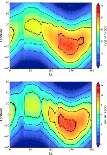
Figure 6. Variability of the LMD-MGCM predicted noon peak limb emission of the CO+
2UV doublet (top left) and the
Cameron bands (bottom left), as a function of latitude and season. Note the different color scale for both panels. Variability of the noon peak altitude of the UV doublet (top right) and the Cameron bands (top left).
we integrate the predicted VERs along the line of sight using limb geometry, taking into account the actual optical path within each atmospheric layer but neglecting horizontal gradients. The variability of the peak intensities is shown in Figure 6. It can be seen that for both emission systems the latitude of the maximum peak intensity moves with the subsolar point, with maximum intensity close to the equator during equinoxes, around 30N for the northern summer solstice and around 30S for the southern summer solstice. Also the peak intensity shows a significant seasonal variability. Intensities at the subsolar point are at maximum (about 75 kR for UV doublet, 430 kR for Cameron bands) around the perihelion season and at minimum (less than 50 kR for UV doublet, close to 300 kR for Cameron bands) around the aphelion season. This is the natural and expected consequence of the high orbital eccentricity of Mars, resulting in significantly more solar photons getting to Mars (and producing increased photoionization and photodissociation) in the perihelion than in aphelion season. Some small departures from this general behavior, such as a period of slightly enhanced emission around Ls =150∘ for the Cameron bands, are also seen.
The variability of the altitude of the peak for both emission systems is also shown in Figure 6. The peak altitude is slightly lower by a couple of kilometers for the CO+
2 UV doublet, but the overall behavior is the same for
both emission systems. Minimum values are found around the aphelion season and maximum values around the perihelion season, due to the seasonal cycle of atmospheric inflation/contraction. In the low latitudes the peak altitudes range from around 115 to 130 km. The altitudes increase when going to higher latitudes (implying higher SZAs), getting maximum values around the polar vortex, due to the increase in the overhead atmospheric column.
Figure 7 shows the contribution of the different processes producing emission in the CO+
2UV doublet, namely
CO2photoionization and CO2electron impact ionization, as a function of latitude and season. Both processes
display similar seasonal evolution, but it can be seen that the emission is clearly dominated at all latitudes and seasons by the CO2photoionization, with the electron impact ionization of CO2representing only a minor contribution. This is in good agreement with previous modeling results (Cox et al., 2010; Evans et al., 2015; Fox & Dalgarno, 1979; Jain & Bhardwaj, 2012; Shematovich et al., 2008; Simon et al., 2009).
Figure 7. LMD-MGCM predicted contribution of the CO2photoionization (top) and the CO2electron impact ionization (bottom) to the emission in the CO+
2 UV doublet at the emission peak, as a function of latitude and season. Note the
different color scale for both panels.
The contribution of the different processes that produce emission in the Cameron bands is shown in Figure 8 (absolute values). While the absolute contribution of the CO2 photodissociation (top left) and the elec-tron impact dissociation of CO2(bottom right) show a latitudinal and seasonal variability similar to the one described above for the CO+
2 UV doublet, the contribution of the electron impact excitation of CO (bottom
left panel) shows a completely different pattern, with several significant increases of emission from a relatively low background at around Ls = 45∘ and from Ls = 120∘ to about 200∘. These increases are so strong that they exceed the otherwise major contributions to this emission system, electron impact dissociation of CO2(top
right), and CO2photodissociation (top left).
4.2. Vertical Profiles at the Subsolar Point
Figure 9 shows the seasonal variability of the limb emission profiles for both emission systems at noon at the subsolar point. The seasonal variability of the peak altitude described above can be clearly appreciated, with peak altitudes for both emission systems varying between about 115 and 130 km. This altitude variability is similar to the one found for the altitude of the main ionospheric peak (see, e.g., González-Galindo et al., 2013), with minimum values around aphelion and maximum values close to perihelion.
It is also important to consider the altitude variability of the contributions of the different processes produc-ing emission in these two systems. The relative contributions for the CO+
2 UV doublet (not shown) are quite
constant during the whole year, with the photoionization of CO2producing around 90% of the emission and
the electron impact ionization of CO2the remaining 10%, with little seasonal and altitude variability.
For the Cameron bands the relative contributions of the different processes can be seen in Figure 10. The situation is, again, more complex than for the CO+
2UV doublet. The contribution of the electron impact
alti-Figure 8. LMD-MGCM predicted contribution of CO2photodissociation (top left), CO2electron impact dissociation (top right), CO electron impact excitation (bottom left), and CO2dissociative recombination (bottom right) to the emission in the Cameron bands at the emission peak.
tude varying between about 20% around aphelion to more than 35% during the second half of the year. Above the peak, the contribution of the CO2electron impact dissociation decreases, oscillating between
about 5 and 15% at an altitude of 160 km. The relative contribution of the electron impact dissociation of CO (bottom left) shows a complex seasonal variability, displaying the strong enhancements of emissions described above. In general, the contribution is larger during the first half of the year than during the second. At the peak altitude, the CO contribution oscillates between around 15% at perihelion to more than 50% dur-ing episodes of enhanced emission in the first half of the year. The contribution of this process increases clearly with altitude above the emission peak at all seasons. This result may have important consequences over the derivation of temperatures from the scale height of the emission (which assumes that CO2is the dominant
factor in this emission) and may explain at least in part why the analysis of the scale heights of the CO+ 2 UV
doublet and of the Cameron bands produces different temperatures (e.g., Leblanc et al., 2006).
Figure 11 shows the predicted variability of the CO volume mixing ratio (vmr). It can be seen that there is a clear correlation between the abundance of CO and the variability of the emission in the Cameron bands produced by photoelectron excitation of CO. Clearly, the periods of enhanced emission are produced by increases in the CO abundance predicted by the model. The thermospheric CO vmr seasonal variability shown in Figure 11 is strongly anticorrelated with the seasonal variability of the thermospheric temperature (not shown). This is expected for a species for which the vertical structure is dominated by molecular diffussion: the ratio of con-centrations between a species lighter than CO2and CO2at a given altitude above the homopause is inversely proportional to temperature (e.g., Houghton, 1986). So, at a given altitude larger relative CO abundances are found during the first half of the year, when the planet is farther away from the Sun and thermospheric temper-atures are colder than during the perihelion season. The sudden decrease in CO abundance at around Ls =60∘ is due to an increase in the temperatures produced by a sudden modification in the dynamical structure pre-dicted by the model. Other factors, such as the CO relative abundance in the lower atmosphere, which is known to present seasonal and latitudinal variations (Sindoni et al., 2011; Smith et al., 2009), are also expected to influence the seasonal variability of CO in the upper atmosphere.
Figure 9. LMD-MGCM predicted variability of the limb emission profile of the CO+
2UV doublet (top) and the Cameron
bands (bottom) at noon at the subsolar point, as a function of Ls. Note the different color scales for both panels.
Previous works have found a significantly smaller contribution of CO photoelectron impact excitation to the emission in the Cameron bands. Shematovich et al. (2008), Simon et al. (2009), Cox et al. (2010), and Jain and Bhardwaj (2012) all show a relative contribution of this process to the Cameron bands emission at the peak that is lower than 10%. In all these works, a neutral atmosphere taken from the Mars Thermospheric General Circulation Model (Bougher et al., 1999, 2006) is used as an input to the dayglow models. As shown in Figure 1 of Shematovich et al. (2008), the relative abundance of CO in the Mars Thermospheric General Circulation Model (appropriate for Ls = 180∘, LT = noon, and Lat = 45∘) is about 2% at 150 km. In contrast, the CO mixing ratio predicted by the LMD-MGCM at this altitude oscillates between about 3.5 and 20%. The larger abundance of CO in the LMD-MGCM explains the larger relative contribution of CO to the emission in the Cameron bands.
It is important to emphasize that the CO abundance variability predicted by the LMD-MGCM still needs to be validated, and thus, we cannot rule out that some of the structures shown in Figure 11 are model arti-facts. Measurements by the Neutral Gas and Ion Mass Spectrometer (NGIMS) mass spectrometer on board MAVEN provided an abundance of about 3–4% of CO at 150 km for the Ls = 288–326∘ season and SZA = 45∘ (Mahaffy et al., 2015, Figures 5 and 6). This is similar to the value predicted by the model at this altitude and time of the year ( 4%), although it also needs to be taken into account that NGIMS CO determinations are affected by uncertainties, since the contribution from CO2fragments and N2needs to be subtracted (Mahaffy
et al., 2015). A detailed comparison with NGIMS abundances obtained at different times of the year is still needed to address if the seasonal variability predicted by the model is realistic or not. In any case, even if the seasonal variability of the contribution to the total emission of the electron impact excitation of CO needs further validation, the increase with altitude of the contribution of this process at any season indicates, once again, that one should be cautious when using the scale height of the Cameron bands to get information about the temperature.
Figure 10. LMD-MGCM predicted profile of the relative contribution to the total Cameron bands emission of the CO2
photodissociation (top left), the CO2electron impact dissociation (top right), the CO electron impact excitation (bottom left), and the CO+
2 dissociative recombination (bottom right) at noon at the subsolar point.
4.3. Geographical and Diurnal Variability of Emission Profiles
We now focus on the VER predicted by the model for both emission systems at three different seasons, rep-resentative of equinox (Ls =0–30∘), northern summer solstice (Ls = 90–120∘, shortly after aphelion), and southern summer solstice (Ls = 270–300∘, shortly after perihelion). Time-averaged results for 30∘ of Ls are analyzed, and the variability of the results with latitude, local time, solar zenith angle, and longitude is studied. The results for the Cameron bands can be seen in Figure 12. For the CO+
2UV doublet the variability is similar
in most respect to that of the Cameron bands, and we do not show it here.
Figure 12. LMD-MGCM predicted variability of VER profiles for the Cameron bands as a function of latitude (left column), local time (center column), and
longitude (right column), for the Ls= 0–30∘(top), Ls= 90–120∘(middle), and Ls= 270–300∘(bottom) seasons. VER = volume emission rate.
The latitudinal variability of the VER profiles for the Cameron bands at noon and at longitude 0 is represented in the left column of Figure 12. For a given season, maximum emission is found close to the corresponding subsolar point. The VER decreases and the peak altitudes tend to increase when departing from the subsolar point. However, there is an exception for the Ls = 270–300∘ season, when the peak altitude decreases when going from the subsolar point to the equator and the low latitudes of the Northern (Winter) Hemisphere. This is produced by the latitudinal variability of the mass density at this season (not shown), which presents at these altitudes a gradient from the denser Northern (Winter) Hemisphere to the less dense southern (summer) pole. This is a consequence of the contraction of the atmosphere due to the lower temperatures close to the surface and is another indication of the importance of fully taking into account atmospheric variability when studying the UV dayglow.
The variability with local time of the VER profile at the equator and longitude 0 for the three seasons is shown in the central column of Figure 12. As expected, maximum emission is obtained at the time of maximum illumination. As before, the altitude of the peak does not always show a symmetric behavior with respect to noon. In particular, for the Ls = 0–30∘ season there seems to be a constant decrease of the peak altitude with increasing local time during the day. Again, this is due to a similar decrease in the atmospheric density at the upper mesosphere/lower thermosphere (not shown). The lower overlying atmospheric column at the end of the day allows deeper penetration of the UV photons.
Finally, the longitudinal variability of the VER profile at the equator and at noon is shown in the right column of Figure 12. A clear longitudinal variability of the peak altitude is found, especially for the Ls = 0–30∘ season.
Figure 13. LMD-MGCM predicted longitudinal variability of the atmospheric density profile (kg/m3) at the equator and
at noon for the Ls= 0–30∘season.
As for the other cases, this is strongly linked to the longitudinal variability of the atmospheric density at these altitudes, shown for the Ls = 0–30∘ case in Figure 13. There is a clear correlation between the variability of the density, apparently dominated by a wave-3 pattern with long vertical wavelength, with that of the peak altitude, with areas of higher density corresponding to higher peak altitude. Longitudinal inhomogeneities attributed to nonmigrating tides have been previously observed in a number of measured quantities in the upper atmosphere of Mars: density measured by accelerometers (Withers et al., 2003), altitude of the iono-spheric peaks (Bougher et al., 2001), NO nightglow (Stiepen et al., 2017), or densities of different species from MAVEN/NGIMS data (England et al., 2016). Wave-2 and wave-3 patterns are usually found to dominate, with the dominant mode depending on the season and latitude of the observations. Especially relevant for this work is the analysis of longitudinal variations in CO2density derived from IUVS measurements of the CO+2UV
doublet (England et al., 2016; Lo et al., 2015). Observations were taken at Ls ≈ 220∘ and Ls ≈ 330∘, respec-tively, in the low latitudes of the Northern Hemisphere. Wave-2 pattern (mainly due to the diurnal eastward 1 tide, DE1) is found to dominate in both studies, with a significant wave-3 contribution (from diurnal east-ward 2, DE2, and semidiurnal easteast-ward 1, SE1, components). In contrast, tidal decomposition of the density field predicted by the model at 130 km shows that, beside the migrating components, the tidal structure
Figure 14. Solar cycle variability of the Cameron bands VER for the Ls= 0–30∘season, as a function of altitude and latitude. VER = volume emission rate.
is dominated by the DE2 component in the low-latitude region, with contribution from the DE1 tide about half that of the DE2 tide. A more detailed comparison with IUVS data, including the tidal structure, is left for a future study.
Regarding the variability with solar cycle, the ratio between the VER for the Cameron bands for the Ls = 0–30∘ season predicted for solar maximum and solar minimum conditions, as a function of altitude and latitude, is shown in Figure 14. This ratio is larger (values between 5 and 6) in the upper layers, decreasing with decreasing altitude as more UV photons are absorbed by the denser atmosphere. At the peak altitude the solar cycle variability of the emission ranges between 2.2 and 2.5, approximately. Similar numbers are obtained for the Ls = 90–120∘ and Ls = 270–300∘ seasons. Note also the weak latitudinal dependence of the ratio. For the CO+
2UV doublet the solar maximum to solar minimum ratio (not shown) is larger than for the Cameron bands,
being around a factor of 2.5–3 at the peak altitude.
5. Summary and Conclusions
A model to simulate two of the most prominent emission systems in the UV dayglow of Mars, the CO Cameron bands and the CO+
2 UV doublet, has been incorporated into the LMD-MGCM. To our knowledge, this is the
first time that a 3-D global atmospheric model has been used to simulate the UV dayglow of Mars, providing a self-consistent coupling of the simulated emissions with the underlying atmospheric variability. As a conse-quence, the first global maps of these emission systems have been produced. The predictions of the model have been tested against four Martian years of SPICAM observations obtained during a period of low solar activity. The following conclusions can be derived from our work:
1. Comparison of the predicted peak intensity of the Cameron bands with SPICAM observations suggests, as in previous works, that a reduction by a factor of 3 in the CO2and CO electron impact excitation cross
sections is necessary to reproduce the observations. The predicted intensity of the CO+
2UV doublet is larger
in about 20% than the observations, within the uncertainty of the associated cross sections.
2. A strong seasonal variability of the peak intensity is predicted by the model but not seen in the observations. Interannual variabilities, not yet considered in the model, may be playing a role.
3. The predicted peak altitude for both emission systems fits well to first order with SPICAM observations, indicating that the model is correctly predicting the atmospheric density in the upper atmosphere. An exception of this good behavior is found for the perihelion season of MY28, a period when a global dust storm developed, where the model underestimates the peak altitude. When including a dust scenario appropriate for MY28, the differences decrease, but do not disappear, indicating that the model may be underestimating the effect of the global dust storm or the aphelion-to-perihelion peak altitude difference. 4. The seasonal variability of the peak emission in the CO+
2UV doublet and the Cameron bands is dominated
by the variability of the Sun-Mars distance produced by the eccentricity of the Martian orbit.
5. For the Cameron bands, a strong contribution of electron impact excitation on CO is found, in particular during the first half of the year. The contribution of this process in our model is significantly larger than in previous 1-D models, due to a larger CO abundance. A significant seasonal variability of this contribution is found, due to seasonal variations in the CO vmr in the upper atmosphere, ultimately linked to predicted temperature variations.
6. The contribution of electron impact excitation on CO to the Cameron bands increases with altitude, indi-cating that one should be cautious when deriving temperatures from the scale height of this emission system.
7. Variability in the geographical and temporal distribution of the atmospheric density induces variability in the simulated dayglow. In particular, the tidal structure of the density in the upper atmosphere is reflected in the variability of the peak altitude of the emission systems.
8. The solar cycle variability of the simulated emission in the Cameron bands is about a factor of 2 at the altitude of the peak, increasing significantly with altitude. The solar cycle variability of the CO+
2UV doublet
is larger than for the Cameron bands.
Some improvements are still possible for the LMD-MGCM including the dayglow model. In particular, although the GCM is able to use a daily varying value of the UV solar flux (González-Galindo et al., 2015), this is not yet possible for the dayglow model. Different strategies are being studied to improve this aspect, decreas-ing at the same time the amount of CPU time consumed by the model, which is significantly larger than when the dayglow model is not used in the GCM.
Comparisons of the model predictions and of the SPICAM observations with the UV doublet and Cameron bands measurements by the IUVS instrument on board MAVEN (Jain et al., 2015) would provide interesting additional information about the variation with the solar cycle and about the seasonal variability of the peak intensities. Similarly, some of the model predictions, such as the longitudinal variability of the dayglow, can-not be confirmed by SPICAM measurements, due to the relatively low number of observations and to the incomplete coverage.
References
Angelats i Coll, M., Forget, F., López-Valverde, M. A., & González-Galindo F. (2005). The first Mars thermospheric general circulation model: The Martian atmosphere from the ground to 240 km. Geophysical Research Letters, 32, L04201. https://doi.org/10.1029/2004GL021368 Avakyan, S., Ii’In, R., Lavrov, V., & Ogurtsov, G. (1999). Collision processes and excitation of UV emission from planetary atmospheric gases: A
handbook of cross sections. Australia, Canada: Gordon and Breach Science Publishers.
Barth, C. A., Hord, C. W., Pearce, J. B., Kelly, K. K., Anderson, G. P., & Stewart, A. I. (1971). Mariner 6 and 7 ultraviolet spectrometer experiment: Upper atmosphere data. Journal of Geophysical Research, 76(10), 2213–2227. https://doi.org/10.1029/JA076i010p02213
Barth, C. A., Hord, C. W., Stewart, A. I., & Lane, A. L. (1972). Mariner 9 ultraviolet spectrometer experiment: Initial results. Science, 175, 309–312. https://doi.org/10.1126/science.175.4019.309
Bell, J. M., Bougher, S. W., & Murphy, J. R. (2007). Vertical dust mixing and the interannual variations in the Mars thermosphere.
Journal of Geophysical Research, 112, E12002. https://doi.org/10.1029/2006JE002856
Bertaux, J.-L., Leblanc, F., Perrier, S., Quemerais, E., Korablev, O., Dimarellis, E., et al. (2005). Nightglow in the upper atmosphere of mars and implications for atmospheric transport. Science, 307, 566–569. https://doi.org/10.1126/science.1106957
Bhardwaj, A., & Jain, S. K. (2009). Monte Carlo model of electron energy degradation in a CO2atmosphere. Journal of Geophysical Research,
114, A11309. https://doi.org/10.1029/2009JA014298
Bhardwaj, A., & Jain, S. K. (2013). CO Cameron band and CO+2UV doublet emissions in the dayglow of Venus: Role of CO in the Cameron band production. Journal of Geophysical Research: Space Physics, 118, 3660–3671. https://doi.org/10.1002/jgra.50345
Bougher, S. W., Bell, J. M., Murphy, J. R., Lopez-Valverde, M. A., & Withers, P. G. (2006). Polar warming in the mars thermo-sphere: Seasonal variations owing to changing insolation and dust distributions. Geophysical Research Letters, 33, L02203. https://doi.org/10.1029/2005GL024059
Bougher, S., Brain, D., Fox, J., Gonzalez-Galindo, F., Simon-Wedlund, C., & Withers, P. (2017). The atmosphere and climate of Mars, Upper
neutral atmosphere and ionosphere (pp. 433–463). Cambridge: Cambridge University Press.
Bougher, S. W., Engel, S., Hinson, D. P., & Forbes, J. M. (2001). Mars Global Surveyor radio science electron density profiles: Neutral atmosphere implications. Geophysical Research Letters, 28(16), 3091–3094. https://doi.org/10.1029/2001GL012884
Bougher, S. W., Engel, S., Roble, R. G., & Foster, B. (1999). Comparative terrestrial planet thermospheres 2. Solar cycle variation of global structure and winds at equinox. Journal of Geophysical Research, 104(E7), 16,591–16,611. https://doi.org/10.1029/1998JE001019 Chan, W. F., Cooper, G., & Brion, C. E. (1993). Absolute optical oscillator strengths for discrete and continuum photoabsorption
of carbon monoxide (7-200 eV) and transition moments for the X1Σ+ →A1Πsystem. Chemical Physics, 170, 123–138. https://doi.org/10.1016/0301-0104(93)80098-T
Chan, W. F., Cooper, G., Sodhi, R. N. S., & Brion, C. E. (1993). Absolute optical oscillator strengths for discrete and continuum photoabsorption of molecular nitrogen (11 200 eV). Chemical Physics, 170, 81–97. https://doi.org/10.1016/0301-0104(93)80095-Q
Cox, C., Gérard, J.-C., Hubert, B., Bertaux, J.-L., & Bougher, S. W. (2010). Mars ultraviolet dayglow variability: SPICAM observations and comparison with airglow model. Journal of Geophysical Research, 115, E04010. https://doi.org/10.1029/2009JE003504
England, S. L., Liu, G., Withers, P., Yi ˇgit, E., Lo, D., Jain, S. S., et al. (2016). Simultaneous observations of atmospheric tides from combined in situ and remote observations at Mars from the MAVEN spacecraft. Journal of Geophysical Research: Planets, 121, 594–607. https://doi.org/10.1002/2016JE004997
Erdman, P. W., & Zipf, E. C. (1983). Electron-impact excitation of the Cameron system (a(3)pi yields x(1) sigma) transition of CO. Planetary and
Space Science, 31, 317–321. https://doi.org/10.1016/0032-0633(83)90082-X
Evans, J. S., Stevens, M. H., Lumpe, J. D., Schneider, N. M., Stewart, A. I. F., Deighan, J., et al. (2015). Retrieval of CO2and N2 in the Martian thermosphere using dayglow observations by IUVS on MAVEN. Geophysical Research Letters, 42, 9040–9049. https://doi.org/10.1002/2015GL065489
Forget, F., Hourdin, F., Fournier, R., Hourdin, C., Talagrand, O., Collins, M., et al. (1999). Improved general circulation models of the Martian atmosphere from the surface to above 80 km. Journal of Geophysical Research, 104(E10), 24,155–24,175.
Fox, J. L., & Dalgarno, A. (1979). Ionization, luminosity, and heating of the upper atmosphere of Mars. Journal of Geophysical Research,
84(A12), 7315–7333. https://doi.org/10.1029/JA084iA12p07315
Furlong, J. M., & Newell, W. R. (1996). Total cross section measurement for the metastable a3Πstate in CO. Journal of Physics B Atomic
Molecular Physics, 29, 331–338. https://doi.org/10.1088/0953-4075/29/2/020
Gagné, M.-E., Bertaux, J.-L., González-Galindo, F., Melo, S. M. L., Montmessin, F., & Strong, K. (2013). New nitric oxide (NO) nightglow mea-surements with SPICAM/MEx as a tracer of Mars upper atmosphere circulation and comparison with LMD-MGCM model prediction: Evidence for asymmetric hemispheres. Journal of Geophysical Research: Planets, 118, 2172–2179. https://doi.org/10.1002/jgre.20165 González-Galindo, F., Bougher, S. W., López-Valverde, M. A., Forget, F., & Murphy, J. (2010). Thermal and wind structure of
the Martian thermosphere as given by two general circulation models. Planetary and Space Science, 58, 1832–1849. https://doi.org/10.1016/j.pss.2010.08.013
González-Galindo, F., Chaufray, J. Y., Lopez-Valverde, M. A., Gilli, G., Forget, F., Leblanc, F., et al. (2013). 3D Martian ionosphere model: I. The photochemical ionosphere below 180 km. Journal of Geophysical Research: Planets, 118, 2105–2123. https://doi.org/10.1002/jgre.20150 González-Galindo, F., Forget, F., López-Valverde, M. A., Angelats i Coll, M., & Millour, E. (2009). A ground-to-exosphere martian general
circulation model: 1. Seasonal, diurnal, and solar cycle variation of thermospheric temperatures. Journal of Geophysical Research: Planets,
114, E04001. https://doi.org/10.1029/2008JE003246
González-Galindo, F., López-Valverde, M. A., Angelat i Coll, M., & Forget, F. (2005). Extension of a Martian general circulation model to thermospheric altitudes: UV heating and photochemical models. Journal of Geophysical Research, 110, E09008. https://doi.org/10.1029/2004JE002312
Acknowledgments
SPICAM L1a data are available in the ESA PSA archive. The model outputs can be requested from F. G. G ([email protected]) and are being currently archived in the UPWARDS catalog within the ESA PSA archive. F. G. G and M. G. C. are partly funded by the European Union Horizon 2020 Programme (H2020 Compet -08-2014) under grant agreement
UPWARDS-633127. M. G. C. was financially supported by the Spanish MINECO through its Ramon y Cajal program. A. Stiepen is supported by the Fund for Scientific Research (F.R.S.-FNRS).
González-Galindo, F., López-Valverde, M. A., Forget, F., García-Comas, M., Millour, E., & Montabone, L. (2015). Variability of the martian thermosphere during eight Martian years as simulated by a ground-to-exosphere global circulation model. Journal of Geophysical
Research: Planets, 120, 2020–2035. https://doi.org/10.1002/2015JE004925
Gronoff, G., Lilensten, J., Simon, C., Barthélemy, M., Leblanc, F., & Dutuit, O. (2008). Modelling the Venusian airglow. Astronomy and
Astrophysics, 482, 1015–1029. https://doi.org/10.1051/0004-6361:20077503
Gronoff, G., Simon Wedlund, C., Mertens, C. J., Barthélemy, M., Lillis, R. J., & Witasse, O. (2012). Computing uncertainties in
ionosphere-airglow models: II. The Martian airglow. Journal of Geophysical Research, 117, A05309. https://doi.org/10.1029/2011JA017308 Houghton, J. T. (1986). The physics of atmospheres (2nd ed.). Cambridge: Cambridge University Press.
Huestis, D. L., Slanger, T. G., Sharpee, B. D., & Fox, J. L. (2010). Chemical origins of the Mars ultraviolet dayglow. Faraday Discussions, 147, 307–322. https://doi.org/10.1039/c003456h
Itikawa, Y. (2002). Cross sections for electron collisions with carbon dioxide. Journal of Physical and Chemical Reference Data, 31, 749–767. https://doi.org/10.1063/1.1481879
Jain, S. K., & Bhardwaj, A. (2011). Model calculation of N 2 Vegard-Kaplan band emissions in Martian dayglow. Journal of Geophysical
Research, 116, E07005. https://doi.org/10.1029/2010JE003778
Jain, S. K., & Bhardwaj, A. (2012). Impact of solar EUV flux on CO Cameron band and CO+2UV doublet emissions in the dayglow of Mars.
Planetary and Space Science, 63–64, 110–122. https://doi.org/10.1016/j.pss.2011.08.010, Advances in Planetary Atmospheres and
Exploration.
Jain, S. K., Stewart, A. I. F., Schneider, N. M., Deighan, J., Stiepen, A., Evans, J. S., et al. (2015). The structure and variability of Mars upper atmosphere as seen in MAVEN/IUVS dayglow observations. Geophysical Research Letters, 42, 9023–9030. https://doi.org/10.1002/2015GL065419
Kirby, K., Constantinides, E. R., Babeu, S., Oppenheimer, M., & Victor, G. A. (1979). Photoionization and photoabsorption cross sections of He, O, N2and O2for aeronomic calculations. Atomic Data and Nuclear Data Tables, 23, 63. https://doi.org/10.1016/0092-640X(79)90021-4 Lawrence, G. M. (1972). Photodissociation of CO2to produce CO(a3Π). The Journal of Chemical Physics, 56, 3435–3442.
https://doi.org/10.1063/1.1677717
Leblanc, F., Chaufray, J. Y., Lilensten, J., Witasse, O., & Bertaux, J.-L. (2006). Martian dayglow as seen by the SPICAM UV spectrograph on Mars Express. Journal of Geophysical Research, 111, E09S11. https://doi.org/10.1029/2005JE002664
Lo, D. Y., Yelle, R. V., Schneider, N. M., Jain, S. K., Stewart, A. I. F., England, S. L., et al. (2015). Nonmigrating tides in the Martian atmosphere as observed by MAVEN IUVS. Geophysical Research Letters, 42, 9057–9063. https://doi.org/10.1002/2015GL066268
Mahaffy, P. R., Benna, M., Elrod, M., Yelle, R. V., Bougher, S. W., Stone, S. W., & Jakosky, B. M. (2015). Structure and composition of the neutral upper atmosphere of Mars from the MAVEN NGIMS investigation. Geophysical Research Letters, 42, 8951–8957. https://doi.org/10.1002/2015GL065329
Montabone, L., Forget, F., Millour, E., Wilson, R. R., Lewis, S., Cantor, B., et al. (2015). Eight-year climatology of dust optical depth on Mars.
Icarus, 251, 65–95. https://doi.org/10.1016/j.icarus.2014.12.034
Montmessin, F., Korablev, O., Lefèvre, F., Bertaux, J.-L., Fedorova, A., Trokhimovskiy, A., et al. (2017). SPICAM on Mars Express: A 10 year in-depth survey of the Martian atmosphere. Icarus, 297, 195–216. https://doi.org/10.1016/j.icarus.2017.06.022
Navarro, T., Madeleine, J.-B., Forget, F., Spiga, A., Millour, E., Montmessin, F., et al. (2014). Global climate modeling of the martian water cycle with improved microphysics and radiatively active water ice clouds. Journal of Geophysical Research: Planets, 119, 1479–1495. https://doi.org/10.1002/2013JE004550
Schunk, R., & Nagy, A. (2000). Ionospheres: Physics, plasma physics and chemistry. UK: Cambridge University Press.
Shematovich, V. I., Bisikalo, D. V., Gérard, J., Cox, C., Bougher, S. W., & Leblanc, F. (2008). Monte Carlo model of electron transport for the calculation of Mars dayglow emissions. Journal of Geophysical Research, 113, E02011. https://doi.org/10.1029/2007JE002938 Simon, C., Witasse, O., Leblanc, F., Gronoff, G., & Bertaux, J.-L. (2009). Dayglow on Mars: Kinetic modelling with SPICAM UV limb data.
Planetary and Space Science, 57(8-9), 1008–1021. https://doi.org/10.1016/j.pss.2008.08.012
Sindoni, G., Formisano, V., & Geminale, A. (2011). Observations of water vapour and carbon monoxide in the Martian atmosphere with the SWC of PFS/MEX. Planetary and Space Science, 59, 149–162. https://doi.org/10.1016/j.pss.2010.12.006
Singhal, R. F., Jackman, C. H., & Green, A. E. S. (1980). Spatial aspects of low- and medium-energy electron degradation in N2.
Journal of Geophysical Research, 85(A3), 1246–1254. https://doi.org/10.1029/JA085iA03p01246
Smith, M. D., Wolff, M. J., Clancy, R. T., & Murchie, S. L. (2009). Compact reconnaissance imaging spectrometer observations of water vapor and carbon monoxide. Journal of Geophysical Research, 114, E00D03. https://doi.org/10.1029/2008JE003288
Stevens, M. H., Evans, J. S., Schneider, N. M., Stewart, A. I. F., Deighan, J., Jain, S. K., et al. (2015). New observations of molecular nitrogen in the Martian upper atmosphere by IUVS on MAVEN. Geophysical Research Letters, 42, 9050–9056. https://doi.org/10.1002/2015GL065319 Stewart, A. I., Barth, C. A., Hord, C. W., & Lane, A. L. (1972). Mariner 9 ultraviolet spectrometer experiment: Structure of Mars’s upper
atmosphere (A 5. 3). Icarus, 17, 469–474. https://doi.org/10.1016/0019-1035(72)90012-7
Stiepen, A., Gérard, J.-C., Bougher, S., Montmessin, F., Hubert, B., & Bertaux, J.-L. (2015). Mars thermospheric scale height: CO Cameron and CO+2dayglow observations from Mars Express. Icarus, 245, 295–305. https://doi.org/10.1016/j.icarus.2014.09.051
Stiepen, A., Jain, S. K., Schneider, N. M., Deighan, J. I., González-Galindo, F., Gérard, J.-C., et al. (2017). Nitric oxide nightglow and Martian mesospheric circulation from MAVEN/IUVS observations and LMD-MGCM predictions. Journal of Geophysical Research: Space Physics, 122, 5782–5797. https://doi.org/10.1002/2016JA023523
Withers, P., Bougher, S. W., & Keating, G. M. (2003). The effects of topographically-controlled thermal tides in the Martian upper atmosphere as seen by the MGS accelerometer. Icarus, 164, 14–32. https://doi.org/10.1016/S0019-1035(03)00135-0
Withers, P., & Pratt, R. (2013). An observational study of the response of the upper atmosphere of Mars to lower atmospheric dust storms.