Dynamic line integral convolution for visualizing electromagnetic phenomena

Dynamic Line Integral Convolution for

Visualizing Electromagnetic Phenomena

by

Andreas Sundquist

Submitted to the Department of Electrical Engineering and Computer Science and to the Department of Physics

in Partial Fulfillment of the Requirements for the Degrees of Bachelor of Science in Physics

Bachelor of Science in Electrical Engineering and Computer Science and Master of Engineering in Electrical Engineering and Computer Science

at the Massachusetts Institute of Technology May 23, 2001

Copyright 2001 Andreas Sundquist. All rights reserved.

The author hereby grants to M.I.T. permission to reproduce and distribute publicly paper and electronic copies of this thesis

and to grant others the right to do so.

Author ________________________________________________________________________ Department of Electrical Engineering and Computer Science, and Department of Physics May 23, 2001 Certified by ____________________________________________________________________ Professor John W. Belcher Thesis Supervisor, Department of Physics Accepted by____________________________________________________________________ Professor Arthur C. Smith Chairman, Department Committee on Graduate Theses, Department of E.E.C.S. Accepted by____________________________________________________________________ Professor David E. Pritchard Senior Thesis Coordinator, Department of Physics

Dynamic Line Integral Convolution for

Visualizing Electromagnetic Phenomena

by

Andreas Sundquist

Submitted to the

Department of Electrical Engineering and Computer Science and the Department of Physics

May 23, 2001

In Partial Fulfillment of the Requirements for the Degrees of Bachelor of Science in Physics

Bachelor of Science in Electrical Engineering and Computer Science and Master of Engineering in Electrical Engineering and Computer Science

Abstract

Vector field visualization is a useful tool in science and engineering, giving us a powerful way of understanding the structure and evolution of the field. A fairly recent technique called Line Integral Convolution (LIC) has improved the level of detail that can be visualized by convolving a random input texture along the streamlines in the vector field. This thesis extends the technique to time-varying vector fields, where the motion of the field lines is specified explicitly via another vector field. The sequence of images generated is temporally coherent, clearly showing the evolution of the fields over time, while at the same time each individual image retains the characteristics of the LIC technique. This thesis describes the new technique, entitled Dynamic Line Integral Convolution, and explores its application to experiments in electromagnetism.

Thesis Supervisor: John W. Belcher

C

ONTENTS

List of Figures ... 5

1

Introduction ... 6

1.1

Dynamic Vector Field Visualization Problem ... 6

1.2 Thesis

Overview ... 7

2 Basic Concepts ... 9

2.1 Notation... 9

2.1.1 Vector Fields ... 9

2.1.2 Streamlines and Path Lines ... 9

2.2 Numerical

Methods... 10

2.2.1 Vector Field Interpolation ... 10

2.2.2 Hermite Curve Interpolation ... 11

2.2.3 Integrating First Order ODEs ... 12

2.2.4 Streamline Integration ... 14

3

Previous Work ... 15

3.1 Line

Integral

Convolution... 15

3.2 Extensions ... 20

3.2.1 Fast Line Integral Convolution... 21

3.2.2 Dynamic Field Visualization... 23

4

Dynamic Line Integral Convolution ... 25

4.1 Problem

Formulation ... 25

4.2 Solution ... 26

4.2.1 Algorithm Overview... 26

4.2.2 Temporal Correlation ... 28

4.2.3 Texture Generation... 30

4.2.4 Particle Advection and Adjustment... 33

4.2.5 Line Integral Convolution ... 37

4.3 Implementation

Details ... 39

4.3.1 Transforming the Fields ... 39

4.3.2 Fast DLIC ... 39

4.3.3 Local Contrast Normalization ... 40

4.4 Alternatives ... 44

4.4.1 Direct Particle Imaging ... 44

4.4.2 Texture Warping... 44

4.4.3 Path Lines ... 45

5.1.1 Definition of a Field Line ... 47

5.1.2 Magnetic Fields ... 48

5.1.3 Electric Fields... 49

5.2

The Falling Magnet ... 50

5.2.1 Experimental Setup ... 50

5.2.2 Computing the Fields ... 51

5.2.3 Equations of Motion ... 53

5.2.4 Results ... 54

5.3 Radiating

Dipole ... 57

5.3.1 Experimental Setup ... 57

5.3.2 Computing the Fields ... 57

5.3.3 Results ... 58

6

Conclusions... 60

6.1 Summary ... 60

6.2 Future

Work ... 60

7 Acknowledgements ... 61

8 References... 62

L

IST OF

F

IGURES

Figure 2-1: Cubic Hermite curve interpolation ... 11

Figure 3-1: Line Integral Convolution applied to a photograph and a spiral vector field... 15

Figure 3-2: Line Integral Convolution applied to random white noise and a spiral vector field ... 17

Figure 3-3: LIC rendering of two electric charges color coded by electric field intensity... 20

Figure 4-1: DLIC animation of a charge moving through a constant electric field ... 25

Figure 4-2: f and d fields of a charge moving against a uniform electric field... 25

Figure 4-3: (s,t) parameterization of a particle’s position via advection along d and f fields... 27

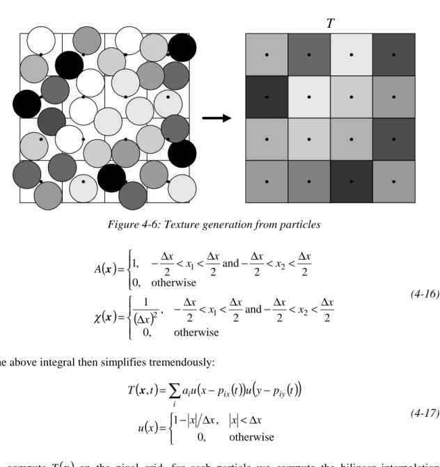
Figure 4-4: Organization of DLIC ... 28

Figure 4-5: Temporal arc-length parameter mapping ... 29

Figure 4-6: Texture generation from particles ... 31

Figure 4-7: Texture coverage ... 34

Figure 4-8: Particle creation... 35

Figure 4-9: Particle merging ... 36

Figure 4-10: Expanding the domain so that the convolutions remain entirely inside ... 38

Figure 4-11: Convolution extent in a circular vector field – shaded by over-sampling... 41

Figure 5-1: Falling magnet experimental setup... 50

Figure 5-2: Animation sequences of the magnet falling through the conducting ring... 56

Figure 5-3: Electric dipole setup ... 57

1 I

NTRODUCTION

In science and engineering, vector fields often play a central role in describing things such as electromagnetism or fluid flow. For the very simplest fields, it is usually possible to analyze its structure on a global scale, and to create a mental image of what it looks like. However, we are often presented with complicated, time-varying fields whose properties are not intuitive or easily analyzable. With the aid of modern technology, we can use computer graphics to create illustrative representations of the vector field, giving us tremendous insight into its structure.

In a fairly recent paper by Cabral and Leedom [3], a general, high-quality method was introduced for visualizing vector fields, called Line Integral Convolution (LIC). A number of papers published thereafter have extended this technique in different ways. One important generalization is to be able to visualize a time-varying vector field, maintaining a natural correspondence between successive frames of the visualization. None of the solutions presented by other researchers can satisfactorily do so for time-varying electromagnetic fields.

This thesis describes a new method called Dynamic Line Integral Convolution (DLIC) developed in conjunction with the TEAL / Studio Physics project that can effectively visualize dynamic electromagnetic fields. It extends LIC by allowing the vector field to vary over time and using a second vector field to describe how the field line structures vary over time. As a result, we have been able to create several animation sequences of experiments in electromagnetism that exhibit all the wonderful detail of the LIC method as well as the evolution of the field over time.

1.1 D

YNAMIC

V

ECTOR

F

IELD

V

ISUALIZATION

P

ROBLEM

Before choosing a method for visualizing vector fields, we need to decide what features of the vector field we would like the image to represent. For example, in some problems only the magnitude of the vector field is important. In this case, a natural representation is to modulate the color/intensity of a pixel on the screen by the magnitude of the vector field at each point. Of course, since a computer display is only a two-dimensional device, this is much more difficult for vector fields of three dimensions of higher.

In other problems, we might instead be interested in the direction of the vector field at each point. Again, we could conceivably modulate the pixel’s color/intensity by the direction of the field. This could even be done for dimensional fields, since a pixel’s color is a

three-dimensional quantity. Unfortunately, color is not a natural way of representing direction. A better solution is to use local directional indicators throughout the vector field. For example, we could establish an ordered grid in a two-dimensional vector field and draw tiny arrows along the direction of the field at those points. The maximum resolution of the visualization is limited, however, because the grid must be coarse enough to provide spacing between the arrows.

Another objective of the visualization may be to observe streamlines (integral lines) in the vector field. One possible solution is to use the above technique to denote the direction at each grid point, and let the observer mentally integrate curves in the vector field. Unfortunately, what the observer perceives is often inaccurate or incomplete, and it is difficult to analyze the features in the field. Instead, we could have the computer automatically integrate along the streamlines and display them. However, this gives rise to the question of which streamlines should be displayed. There are methods for automatically selecting a reasonable distribution of streamlines, but they cannot guarantee that all the important features will be represented. Fortunately, texture-based methods such as LIC are straightforward and robust alternatives that faithfully represents the streamlines with as much detail as possible.

Finally, extending the visualization to dynamic fields creates a new set of challenges. In some applications, it might suffice to render each frame independently via one of the previous techniques, in which case the solution is straightforward. However, other problems, including electromagnetism, have complex inter-frame dependencies since we expect to be able to understand how field lines evolve over time. Thus, one difficulty is how to describe the correspondence between vector field points or streamlines over time in the first place. Once we have defined their motion, we face the challenge of producing an animation sequence that depicts this evolution in an intuitive fashion. Another problem is maintaining a consistent level of detail throughout the image, even as streamlines are compressed and expanded. LIC by itself cannot be used in general for time-varying vector fields, since it does not use any information about how the field lines move, nor does it attempt to maintain any sort of inter-frame coherence. The DLIC method introduced here offers a solution to these challenges.

1.2 T

HESIS

O

VERVIEW

This thesis is organized into four major sections. Chapter 2 introduces the basic concepts that are needed to discuss vector fields, streamlines, and some of the computational methods used

Convolution technique and some of its important improvements, as well as other attempts to extend the method to dynamic vector fields. Chapter 4 describes the new Dynamic Line Integral Convolution algorithm and some of the details of our implementation. Finally, chapter 5 illustrates the application of DLIC to two experiments in electromagnetism.

2 B

ASIC

C

ONCEPTS

In this chapter, some of the fundamental ideas used in vector field visualization will be introduced, along with some practical computational techniques.

2.1 N

OTATION

2.1.1 V

ECTOR

F

IELDS

We define a vector field f as a function mapping a Euclidean domain D⊂Rn to another space R of the same dimension: n

(

)

n R y D x f ∈ = ∈ (2-1)

For our purposes, we only use two- and three-dimensional vector spaces, since higher dimensions are not natural to visualize.

For time-dependent vector fields, we write f as a function mapping D×T to Rn, where

T is some scalar time interval:

(

_{x D t T}

)

_{y R}n

f ∈ , ∈ = ∈ (2-2)

2.1.2 S

TREAMLINES AND

P

ATH

L

INES

A streamline 1 is defined as an integral curve in a stationary vector field:

( ) ( )

f 1 , 1

( )

0 10

1 u = u = du

d

(2-3)

In this case, the magnitude of the vector field determines how 1 is parameterized. We can reparameterize the curve by arc length s to obtain 1ˆ :

( )

( )

f

( )

1 f 1 f 1 1 f ⇒ ˆ = = ˆ = ˆ ˆ = ds du du d s ds d du ds (2-4)

Care must be taken, as this parameterization breaks down where the vector field vanishes. The notation 1ˆ_x

( )

s will often be used to indicate the streamline for which 1ˆ_x

( )

0 =x.

For time-dependent vector fields, a streamline is similarly defined at a constant time:

( ) ( )

f 1, 0 , 1

( )

0 10

1 u = t u = du

d

( ) ( )

( )

0 0 0 0 0 0 0 1 f 1, , 1 1 1 1 = t = u t t du d , (2-6) where

( )

₀ 0 1 1u

t indicates the streamline seeded at 1 when 0 u=0 at the constant time t . 0

Note that this is different from a path line, which is an integral path taken over time:

( ) ( )

f , , 

( )

0 0

t = t t = dt

d

(2-7)

Again in chapter 4, an alternative notation will be used for such an integral path:

( ) (

_{0 0}

)

0

( )

_{0 0} 0 0  f , ,     = + t = t t t t dt d , (2-8) where

( )

₀ 0  t

t is the path line seeded at  at time 0 t0 when t=0.

2.2 N

UMERICAL

M

ETHODS

2.2.1 V

ECTOR

F

IELD

I

NTERPOLATION

In computer programs, vector fields are often represented as samples over a discrete grid, either as a result of a grid-based field computation method or as a way to speed up vector field evaluations. In order to reconstruct the continuous field function, a number of different interpolation methods can be employed. A general technique is to convolve the discrete samples with a continuous kernel. For example, on a two-dimensional integer grid g

{ }

i,j with a kernel

( )

x,y

χ we define the vector field f by:

( )

x,y =

_∫∫

g

{



x+x′

 

, y+y′



} (

χ x′,y′

)

dx′dy′

f (2-9)

For our purposes, bilinear interpolation is sufficient because the vector fields are generally smooth. The bilinear convolution kernel in two dimensions is:

( )

   < < < < = otherwise , 0 1 0 and 1 0 , 1 ,y x y x χ (2-10)

The resulting expression for the vector field simplifies to

( )

,

(

1

) (

(

1

)

g0,0 g1,0

)

(

(

1

)

g1,0 g1,1

)

f x y = −y_f −x_f +x_f +y_f −x_f +x_f , where (2-11)

 

x y y

 

y

{

 

x m

 

y n

}

x

This expression can be evaluated very quickly.

2.2.2 H

ERMITE

C

URVE

I

NTERPOLATION

Another place that interpolative methods are useful is for reconstructing a continuous streamline from discrete samples. Suppose we have a sequence of samples parameterized by arc length:

( ) ( ) ( )

s 1 s 1 s 1

( )

sn

1ˆ ₀ , ˆ ₁, ˆ ₂ ,..., ˆ (2-13)

In addition to the position, we know the tangent of the curve at those parameters from the vector field:

( )

sk

(

( )

sk

)

ds d 1 f 1ˆ = ˆ ˆ (2-14)

Between two adjacent sample points k and k+1, we can fit a cubic Hermite curve by using the two positions and the two tangents:

( )

[

]

( )

( )

( )

(

)

( )

(

)

k k k k k k k k s s h h s s s s h s h s s s s s s − = − = ′                         − − − − ′ ′ ′ = + + + 1 1 1 2 3 , ˆ ˆ ˆ ˆ ˆ ˆ 0 0 0 1 0 1 0 0 1 2 3 3 1 1 2 2 1 ~ 1 f 1 f 1 1 1 (2-15)

This curve has the desired properties at the endpoints

( ) ( )

( ) ( )

( )

(

( )

)

( )

1

(

( )

1

)

1 1 ˆ ˆ ~ , ˆ ˆ ~ , ˆ ~ , ˆ ~ + + + + = = = = k k k k k k k k k k k k s s ds d s s ds d s s s s 1 f 1 1 f 1 1 1 1 1 (2-16)

and smoothly interpolates between the sample points as we’d expect, illustrated in Figure 2-1.

( )

sk 1ˆ

( )

1 ˆ s_k+ 1

( )

(

1 sk

)

f ˆˆ

( )

(

ˆ 1

)

ˆ + k s 1 f

Unfortunately, even though the tangents at the endpoints are unit magnitude, in general this will not be true in between. However, as long as the streamline does not vary excessively between two successive sample points, Hermite curves are a good approximation. In addition, because a Hermite curve is a cubic polynomial, it can be evaluated at equi-spaced points along s very quickly using forward differences. First, the initial values of four variables are computed:

( )

(

(

)

)

( ) ( ) (

)

( ) ( )

(

) (

)

( )

3 3 2 1 0 1 2 3 0 1 2 2 3 3 6 , 2 ~ ~ 2 ~ , ~ ~ ~ a d 1 1 1 d 1 1 d a a a a a a a a 1 s s s s s s s s s s s s s s s s s s ∆ = ∆ ∆ − + ∆ − − = ∆ − − = + + + = + + + =

Then, we can compute the next sample point in succession with only three additions:

(

) ( )

(

)

(

)

( )

(

)

(

)

d

( )

d d d d d d 1 1 ∆ + = ∆ + ∆ + + = ∆ + ∆ + + = ∆ + s s s s s s s s s s s s s 2 2 2 1 1 1 ~ ~ (2-17)

2.2.3 I

NTEGRATING

F

IRST

O

RDER

ODE

S

In scientific computing, one of the most basic types of problems is integrating first order ordinary differential equations. Given the differential equation and initial condition

( )

x, , x

( )

0 x0 f x = = t t dt d , (2-18)

how do we compute the value of x

( )

t₁ ? If the vector field f is continuous and satisfies the Lipschitz condition, then a unique solution exists. Often, this is not the case, and care must be taken to understand the consequences of picking one particular solution over another.

Most methods for evolving the system by the required time step t₁−t₀ use one-step or multi-step techniques. The simplest possible (and also the least accurate) is the Simple Euler method. To evolve the system by a time step h, we use the rule:

( ) ( )

t h x t hf

(

x

( )

t,t

)

x + = + (2-19)

A much more accurate and robust technique devised by Runge and Kutta is the standard RK4 integrator, which uses four evaluations of f to estimate the next step:

( ) ( )

[

]

( )

(

)

( )

(

)

( )

(

)

( )

(

t h t h

)

h t h t h t h t t t h t h t c d b c a b a d c b a + + = + + = + + = = + + + + = + , 2 , 2 2 , 2 , 2 2 6 f x f f f x f f f x f f x f f f f f f x x (2-20)

Although there are more sophisticated, higher-order methods for integrating ODEs, such as the Adams predictor-corrector methods, the added complexity does not provide significant gains for our application. Indeed, for the fourth-order RK4 method the error goes as O

( )

h5 , so to obtain the desired accuracy we can simply reduce the step size h.

If we have an implicit equation for the exact integral curve (for example, as a result of a potential function), then we can use it to automatically adjust the step size to keep the results of the integrator within the desired error tolerance. Or, we can more generally construct an error metric by comparing the results of two integrators of different order. As discussed in Stalling dissertation [19], Fehlberg came up with a technique to use the intermediate results of the RK4 integrator to construct a third-order result to be used as an error estimate:

(

) ( )

[

(

(

)

)

]

(

t h

) (

t h

)

h

(

(

t h

)

)

h t h t h t d c b a + − = + − + = + + + + + = + x f f x x x f f f f x x 6 ~ 2 2 6 ~ ε (2-21)

Given an error tolerance ε_tol, and knowing the error goes as O

( )

h5 , we can estimate the largest step size h* that will remain within the tolerance as

        =min 5 , max * h h tol ε ρε , (2-22)

where ρ < 1 is a safety factor to compensate for higher-order errors. The step size needs to be limited to a maximum of h_max since the error can become arbitrarily small. When a step is taken whose error is too large, the step size h is adjusted to h* and the step is recomputed. When the step taken falls within the error tolerance, the next step is computed with the new step size h*. This way, the integrator’s performance is maximized by taking the largest steps possible.

2.2.4 S

TREAMLINE

I

NTEGRATION

When the adaptive error-controlled RK4 integrator is combined with a cubic Hermite polynomial interpolator, the result is a fairly robust and efficient method for producing samples spaced evenly along a streamline 1ˆ . To summarize the algorithm:

1. Starting at the initial point 1ˆ s

( )

₀ , use the adaptive error-controlled RK4 on the unit-magnitude vector field to produce a sequence of sample points and their parameters:

( ) ( ) ( ) ( )

, ˆ , ˆ , ˆ ,... ˆ s₀ 1 s₁ 1 s₂ 1 s₃

1

2. For each equi-spaced point s₀+n∆s, let k_n be the index of the integrator sample point immediately preceding it (i.e. ≤ ₀+ ∆ < ₊₁

n

n k

k s n s s

s ). Compute the sample point by fitting a cubic Hermite polynomial to the integrator points ˆ

( ) ( )

,ˆ ₊₁

n

n k

k s

s 1

1 and the tangents

( )

( ) ( )

ˆ , ˆ

(

ˆ 1

)

ˆ + n n k k s s f 1 1

f . A contiguous subsequence of equi-spaced points between two adjacent integrator sample points should be computed quickly via forward differences. The result is another sequence:

( ) (

,~

) (

,~ 2

) (

, ~ 3

)

,... ~ 0 0 0 0 s s s s s s s 1 +∆ 1 + ∆ 1 + ∆ 1

With these more or less evenly spaced samples, we can approximate line integrals taken along streamlines. For example, the line integral over the scalar field r:D→R can be approximated as a discrete sum:

( )

( )

_∑

(

(

)

)

∫

≅∆ + ∆ n s n s r s ds s r 1ˆ 1~ ₀ . (2-23)

A line integral convolution can be computed similarly:

(

)

[

⊗

]( )

=

_∫

(

(

+

)

) ( )

≅∆

_∑

(

(

+ ∆

)

) ( )

∆ n s n s n s r s ds s s s r s r$1ˆ κ ₀ 1ˆ ₀ κ 1~ ₀ κ~ , (2-24)

where κ~

( )

s is a discrete approximation of the convolution kernel κ

( )

s . Note that the kernel should have a limited extent in order for the summation to be feasible.

A streamline integrator is not complete if it does not deal with streamline abnormalities, however. For example, what is the correct behavior when the streamline leaves the vector field domain D or terminates in a sink? What should the integrator do if the vector field does not obey the Lipschitz condition, and there isn’t a unique solution? These questions can only be answered by examining the particular problem at hand.

3 P

REVIOUS

W

ORK

3.1 L

INE

I

NTEGRAL

C

ONVOLUTION

In a seminal paper published by Cabral and Leedom entitled “Imaging Vector Fields Using Line Integral Convolution” [3], a new technique was introduced that allows us to represent vector fields with a level of detail as fine as the pixels on a computer screen, without causing confusion by being so densely packed. Line Integral Convolution (not to be confused with merely convolving via a line integral) can be viewed as an operation on an input texture and a vector field to produce an output image that represents the field.

Ideally, we can describe the result of this operation as:

( ) (

=

[

T

)

⊗

]

( )

=

_∫

T

(

( )

s

) ( )

s ds

I x $1ˆ_x κ 0 1ˆ_x κ , (3-1)

where I

( )

x is the output image intensity at the continuous location x, T

( )

x is the input texture intensity at x, κ

( )

s is the convolution kernel, and 1ˆ_x

( )

s is the arc-length parameterized streamline such that 1ˆ_x

( )

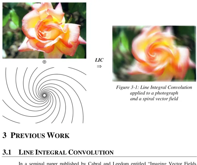
0 =x. The above Figure 3-1 was generated by applying LIC separately to each of the red, green, and blue color components of the color photograph, using a constant

⊕ LIC

⇒

Figure 3-1: Line Integral Convolution applied to a photograph and a spiral vector field

convolution kernel of finite extent. We can see that the image has been “blended” along the direction of the spiral vector field.

One interesting effect of this operation is the correlation between output intensities along the same streamline, for example between x and 1ˆ_x

( )

∆s . The integral for the intensity at 1ˆ_x

( )

∆s can be rewritten as:

( )

(

)

(

_{( )}

( )

)

( )

(

(

)

) (

(

)

)

( )

(

) (

)

∫

∫

∫

′ ∆ − ′ ′ = ∆ − + ∆ + ∆ = = ∆ _∆ s d s s s T ds s s s s s T ds s s T s I _s κ κ κ x x 1 x 1 1 1 1 _x ˆ ˆ ˆ ˆ _ˆ (3-2)

This identity uses the fact that 1_{1 ( )∆s}

( )

s =1_x

(

∆s+s

)

x ˆ

ˆ_ˆ . The resulting difference in intensity can therefore be expressed as:

( )

(

∆s

) ( )

−I =

_∫

T

(

( )

s

) (

[

s−∆s

) ( )

− s

]

ds

I 1ˆ_x x 1ˆ_x κ κ (3-3)

If the difference between κ and itself shifted by ∆s is small, then the output intensities will be very similar.

For a two-dimensional field, in order to compute the output intensity of a particular pixel

0

x , ideally we would convolve I

( )

x with the spatial response curve χ

( )

x of a pixel:

( )

x =

_∫∫

I

(

x +x

) ( )

x dx

O _{0 0} χ (3-4)

Using something like a radially-symmetric Gaussian response curve would give high-quality results, but computing the full integral is too time-consuming. In practice, if the input texture

( )

x

T comes from pixels with a resolution at least as coarse as O

( )

x , then I

( )

x will have frequency components that are only as high as those in T

( )

x . Therefore, we can get results that are almost as good by using a much simpler filter. For example, we could use a constant response curve

( ) ( )

    ₋∆ _{< <}∆ ₋∆ _{< <} ∆ ∆ = otherwise , 0 2 2 and 2 2 , 1 2 1 2 x x x x x x x x χ (3-5)

where x∆ is the width and height of a square pixel. Usually, it is simplified even further by approximating the convolution integral as the sum of a few samples; often even a single sample will suffice.

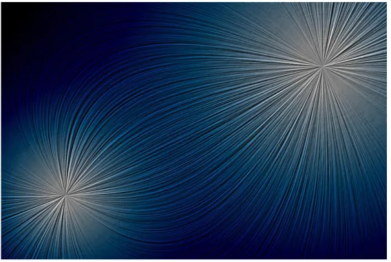
Though the LIC technique can be viewed as an image operator, in order to visualize vector fields, random white noise is typically used as the input texture. This way, the net effect of LIC is that output intensities along a streamline tend to vary very slowly in intensity, while pixels in the perpendicular direction have no correlation. Thus, an observer can easily discern the direction of the vector field – an example can be seen in Figure 3-2. Although the above description of LIC has focused on two-dimensional vector fields, the method extends naturally to higher dimensions. In particular, three-dimensional fields can be successfully imaged, although it is more difficult to present the results on a two-dimensional computer display.

Images produced in this way have a strong resemblance to particle streak images produced by real-life flow experiments. The reason is because the input texture can be viewed as an instantaneous image of the particles at one point in time, and the consequent application of LIC spreads the particles along their streamlines via the convolution kernel κ

( )

s . The following discussion of the particle image-formation process is similar to the model described in Stalling’s dissertation [19]. For one particle, given its initial position p_i

( )

0 , we can describe its advection path as:

( )

t ( )

( )

t i i 1p 0 p = (3-6) ⊕ LIC _⇒

Figure 3-2: Line Integral Convolution applied to random white noise

Suppose the particle has an intrinsic intensity level a , and that over time its “exposure” on the _i output image is proportional to κ

( )

t . Then, the resulting image due to that particle is:

( )

=

_∫

a

(

−

( )

t

) ( )

t dt

I_i x _iδ x p_i κ , (3-7)

where we represent the image of the particle via a delta-function. Taking the contributions of all the particles together, the output image is:

( )

=

∑

( )

=

∑∫

(

( )

−

) ( )

=

∑∫

(

( )

( )

−

)

( )

i i i i i i i a t t dt a t t dt I I i κ δ κ δ p x 1 x x x _{p 0} (3-8)

Now, suppose all the particles at time t=0 densely cover the domain D. Then, we can turn the sum over the particles into an integral over D:

( )

=

_∫∫

(

( )

t −

)

a

( )

t dtd =

_{∫ ∫}

(

( )

t −

)

a

( )

t d dt I D y x 1 y x 1 x _{y y} D y y κ δ κ δ (3-9)

where a is the intensity of the particle that is at y at time _y t=0. Assuming the particle paths are unique, the delta function is non-zero when:

( )

t = ⇔ = _x

( )

−t

y x y 1

1 (3-10)

In order to integrate out the delta function, we need to consider what happens as we vary the integration variable y near the point where the delta function is non-zero. If we vary y an amount ε along the direction of the streamline, then 1y

( )

t will move by an amount

        ⋅ − t dt ds dt ds 1 0 ε , (3-11)

where s is the arc-length along the streamline. Similarly, if we vary y in a direction perpendicular to the streamline, 1_y

( )

t will also move, scaled some relative expansion or contraction of the streamlines. This can be an extremely complicated effect, and so I will simply denote it by the symbol β. Thus, taking these variances into account, we can integrate out the delta function and rewrite the intensity of a point as:

( )

∫

_               ⋅ = − − _dt dt ds dt ds t a I t 1 0 1 ) (x _yκ β , (3-12)

( )

(

) ( )

∫

_               − = − − _dt dt ds dt ds t t T I t 1 0 1 ) (x 1_x κ β (3-13)

If we parameterize the particle paths by distance instead of time, then we would have s

t= and ds dt=1, which would dramatically simplify the equation. Indeed, this is desirable if we are more interested in the direction of the vector field than the magnitude. Finally, although β may have a strong effect on the intensity, for visualization purposes it makes sense to set this to one. For example, a large β means that the streamlines have “spread apart”, and that the particles have a overly small effect on the output intensity. I argue that particles should not be affected by how the streamlines expand and contract, but that their advection should simply represent the directions of the streamlines. Finally, reversing the direction of the integral, the result is the expression:

( )

=

_∫

T

(

( )

s

) ( )

−s ds

I x 1ˆ_x κ (3-14)

This is identical to the output intensity function for Line Integral Convolution, if κ

( ) ( )

s =κ −s . Intuitively, the above particle-advection model can be seen as “scattering” the particles along their streamlines, while Line Integral Convolution “gathers” particles along the streamlines that would have contributed to each output point.

Typically, as discussed earlier, streamlines used in LIC are reparameterized by arc-length, which is important in order to control the degree of streamline correlation and maintain a consistent level of detail despite large variances in the vector field magnitude. Unfortunately, information about the vector field’s magnitude is by this reparameterization. A simple method for reintroducing this information is color-coding the output intensities by the local field magnitude, as seen in Figure 3-3. Another technique due to Kiu and Banks [12] uses multiple input textures with different frequency extents, blending them according to the local vector magnitude. This results in images that have very coarse detail where the magnitude is small and fine detail where the magnitude is large (or vice versa).

3.2 E

XTENSIONS

A number of papers published after the introduction of LIC have extended it in important ways. In the article “Fast and Resolution Independent Line Integral Convolution” by Stalling and Hege [18], a method was described to decouple the input and output resolutions, and also to accelerate the LIC computation by an order of magnitude for box-filter convolutions. We can make the output resolution independent of the input resolution simply by introducing a transformation ΦΦ from the output pixels O

( )

x to the output intensity field I

( )

x :

( )

x =

_∫∫

I

(

-

(

x +x

)

) ( )

x dx

O _{0 0} χ (3-15)

Indeed, we could also have separate coordinate systems for the input texture and the vector field. For example, if the input texture is made coarser than the vector field, then the resulting output image will be a coarser rendition of the vector field. In her paper “Visualizing Flow Over Curvilinear Grid Surface Using Line Integral Convolution” [6], Forsell extended it further, allowing LIC to work on more general surfaces.

A number of other methods have been developed whose results are similar to those achieved by the LIC method. For example, the concept of “splatting” was used to visualize vector fields by Crawfis and Max [4] and similarly by de Leeuw and van Wijk [14]. Another paper by de

Figure 3-3: LIC rendering of two electric charges color coded by electric field intensity

Leeuw and van Liere, “Comparing LIC and Spot Noise”[13], describes how the two relate, while Verma, Kao, and Pang attempt to consolidate LIC with the idea of drawing streamlines in their article on a hybrid method called Pseudo-LIC [20]. Wegenkittl, Gröller and Purgathofer use an asymmetric LIC convolution kernel in order to provide additional information about the orientation of the vector field in their paper on Oriented Line Integral Convolution [21]. Surprisingly, a radically different diffusion method developed by Diewald, Preußer, and Rumpf [5] produces results very similar to LIC – in fact they claim it is more general than LIC. Also, there exist several methods for approximating LIC in order to speed it up substantially. For example, the document “Adaptive LIC Using a Curl Field and Stochastic LIC Approximation using OpenGL” by Bryan [2], takes advantage of hardware acceleration.

3.2.1 F

AST

L

INE

I

NTEGRAL

C

ONVOLUTION

Returning to the paper by Stalling and Hege on Fast Line Integral Convolution (FLIC) [18], suppose that the convolution kernel κ

( )

s takes on the form:

( )

    _{− < <} = otherwise , 0 , 2 1 S s S S s κ (3-16)

Then, there is an interesting relationship between the output intensities of two points along a streamline separated by ∆s<2S:

( )

(

) ( )

(

( )

) (

[

) ( )

]

( )

(

)

(

( )

)

        − = − ∆ − = − ∆

∫

∫

∫

∆ + − − ∆ + S s S s S S ds s T ds s T S ds s s s s T I s I x x x x 1 1 1 x 1 ˆ ˆ 2 1 ˆ ˆ κ κ (3-17)

Next, we turn the continuous integrals into discrete sums taken with a step size of s∆ , using the discrete version of the convolution kernel:

( )

    _{− ≤ ≤} + ∆ = ∆ otherwise , 0 , 1 2 1 N n N s N s n κ (3-18)

The relationship between adjacent output intensities along the streamline becomes much simpler:

( )

(

) ( )

(

( )

) ( )

[

(

) ( )

]

(

)

(

)

(

)

(

(

)

)

[

T N s T N s

]

s N s n s n s n T I s I n ∆ − − ∆ + + ∆ = ∆ − ∆ − ∆ ≅ − ∆

∑

x x x x 1 1 1 x 1 ˆ 1 ˆ 1 2 1 ~ 1 ~ ˆ ˆ κ κ (3-19)

Thus, we can incrementally compute the output intensities along a streamline in constant time per step. In fact, this method can be extended to speed up piece-wise polynomial convolution kernels as well [10] [19].

In the original LIC algorithm, the discrete convolution that produces the output pixels

( )

x0

O dictates which output intensity points I

( )

x are computed. For the Fast LIC algorithm, in order to take advantage of the above relationship, we cannot insist on sampling the output intensities according to the discrete convolution filter χ

( )

x . In fact, if we pick random starting points for the incremental streamline convolutions, the resulting set of output intensity samples are themselves pseudo-randomly distributed.

However, consider the convolution filter

( )

_∑

(

( )

)

= − = 0 0 0 0 1 1 x x x x x x z N i i N δ χ , (3-20)

which is specific to each output pixel x . The number of samples ₀ Nx₀ is small, and the sample

locations ( )i

0

x

z are scattered randomly around the pixel center. As is well known in computer graphics, as long as the frequency components in I

( )

x are not higher than the frequencies that can be represented by O

( )

x₀ , a random sampling gives a reasonable approximation to a continuous convolution with a kernel proportional to the probability density of the sample points. Therefore, given a set of samples I x , the uniform square convolution kernel (Equation 3-5)

( )

_i can be approximated by accumulating each sample in the appropriate output pixel, and then dividing each output pixel by the number of samples that hit it.

Thus, FLIC is typically implemented as follows:

1. Pick a random sample point x and compute I

( )

x by a discrete streamline convolution. Accumulate this result in the appropriate output pixel.

2. Produce a sequence of new sample points I

(

1ˆ_x

( )

k∆s

)

via the incremental method and accumulate those pixels. Continue along the streamline for some maximum distance M∆s.

3. If “most” of the output pixels have been hit at least as often as some specified minimum, then continue to the next step. Otherwise, go back to step 1.

4. For the remaining pixels that have not been hit often enough, sample the output intensity at those pixels and accumulate the result until every pixel has been hit the minimum amount.

5. Normalize the output pixels by dividing out the number of samples that have hit each pixel.

This algorithm produces results that are almost the same as those produced by LIC. For a streamline convolution of length N∆s, if we follow it for a distance M∆s, the ratio between the number of input textures sampled for LIC and for FLIC is roughly

( )

N M N M N θ θ ≈      + ⋅ , (3-21)

where M is typically some factor larger than N. Since the cost of computing one streamline convolution is amortized over the entire length that the streamline is followed incrementally, FLIC achieves an order of magnitude speed-up.

Note the one downside of FLIC is that its results are somewhat dependent on how the streamlines are sampled. Two different random samplings will produce variations in the output images that are distinguishable upon careful examination. Thus, if the same vector field (or one that is similar) is to be visualized more than once using FLIC, care must be taken to preserve the order of the sampling.

3.2.2 D

YNAMIC

F

IELD

V

ISUALIZATION

There have been a number of articles describing methods for animating vector field images in the style of LIC. Most of them fall into one of two categories: depicting cyclic motion along streamlines for static vector fields, or simulating fluid motion along the streamlines of time-dependent flow fields.

The original paper by Cabral and Leedom on LIC [3] described a method for animating the field lines in the direction of the vector field by varying the convolution kernel over time. This method is based on a technique first described by Freeman, Adelson, and Heeger in “Motion Without Movement” [8]. By shifting a pseudo-periodic kernel in space over time, the output image appears to move along the direction of the kernel translation, in this case along the field lines. Jobard and Lefer reduced the time it takes to render an animation sequence by precomputing a “motion map”, from which all the frames can be quickly extracted [11]. Forssell and Cohen improved LIC for variable-speed animation on curvilinear grids [7].

Other research has been done that allows the vector field itself to vary over time, but the application has almost always been fluid-flow models. In the same paper by Forssell and Cohen [7], they describe a modification to LIC whereby streaklines instead of streamlines are followed, where streaklines are defined as the set of points that pass through a seed point when advected through time. Unfortunately, because convolutions are performed over space as well as time, images exhibit behavior that looks “ahead” in time, which is unphysical and can be misleading. Shen and Kao modify this algorithm by feeding forward advected streakline paths and the results of the convolution instead of using future streakline immediately in their two publications on Unsteady Flow LIC [16] [17].

Evidently, vector field visualization techniques are most often used in flow problems, where the field indicates the direction of flow. Thus, the very same vector field that is being visualized also indicates how it should “flow” over time. In electromagnetism, this is no longer the case. We are visualizing electric or magnetic fields, but their “motion” is not generally along the field lines – in fact, motion along streamlines has no meaning. Visualizing electromagnetic fields presents us with a more general problem than that of visualizing fluid flow, since the vector field and the “motion” of the vector field lines themselves are different.

4 D

YNAMIC

L

INE

I

NTEGRAL

C

ONVOLUTION

4.1 P

ROBLEM

F

ORMULATION

Given two time-dependent vector fields f,d:D×T→Rn, where f is the vector field we would like to visualize, and d describes how its field lines evolve over time, how do we generate a sequence of images that represents this information effectively? The field f is the same as before, except that it is allowed to vary over time, while the new field d is the instantaneous velocity of the motion of every streamline point in f. The sequence of images must intuitively depict the streamlines in f evolving over time as indicated by d. Each individual image must by itself be an accurate and detailed representation of the vector field f at a particular time. When viewed as a sequence, it should be clear how its streamlines evolve over time. Figure 4-2 below is an example of the two fields for an electric charge moving against a uniform electric field.

At this point, the notation 1ˆ_ts

( )

x will be used to specify streamlines in f at constant time t Figure 4-1: DLIC animation of a charge moving through a constant electric field

f vector field: the background vertical field

lines “bend” around the electric charge

d vector field: as the charge moves down, the

field lines are “pushed” apart horizontally, and near the charge move down along with it

seeded at x and parameterized by arc-length s, while _t∆t

( )

x will denote path lines in d starting at

x at time t, evolved by a time delta t∆ . Assuming the streamlines are all unique and can be labeled by some parameter . , every point must move such that

( )

. x d

( )

x 1

( )

. 1

x= ˆ_ts ⇒ + ,t dt= ˆ_ts₊′_dt , (4-1) for some parameters s and s′ and an infinitesimal time delta dt. In other words, a point x must move with a velocity specified by d to another point on the same streamline at a different time.

It may seem that d and f encode redundant information, or that the above condition is excessively constrained. Indeed, for an n-dimensional domain D⊂Rn, we could label the streamlines by an

( )

n−1 -dimensional parameter . , and thus a function d:Rn−1×T →Rn−1

could describe the evolution of the streamlines over time. However, not only is this representation very difficult to work with, it does not specify how different points on a particular streamline evolve along the streamline. Using two fields f and d is a straightforward way of representing all the information.

Note that fluid flow visualization becomes a subclass of this problem, where we take

f

d= . Since the streamlines visualized in f depict the direction of flow, it can likewise be used to describe how particles move along streamlines.

4.2 S

OLUTION

The solution presented in this thesis, called Dynamic Line Integral Convolution, allows us to visualize time-varying vector fields represented by the f and d fields described above. Although it makes use of the LIC algorithm to render the images, the method is actually more general in that other texture-based vector visualization techniques could be used as well. Figure 4-1 is an example of DLIC, which shows a sequence of images of a charge moving against a uniform electric field.

4.2.1 A

LGORITHM

O

VERVIEW

Conceptually, the technique employed by DLIC is fairly simple. Going back to the model of the particle image-formation process in Equation 3-7, the output intensity can be seen as a sum of contributions from a number of particles:

( )

=

_∑∫

(

−

( )

) ( )

i

i i s a s ds

I x δ x p κ (4-2)

Now, instead of interpreting the streamlines in f physically as the motion of particles over time, we think of it simply as an imaging effect. Instead, we allow the particles to advect over time in the d field:

( )

t

( )

i i t  p

p = ₀ (4-3)

At any particular time, we form streamlines that are seeded at the location of the particle at that time:

( )

ts

(

i

( )

)

ts

(

t

( )

i

)

i s t 1 p t 1  p

p , = ˆ = ˆ ₀ (4-4)

Thus, the image-formation process over time can now be described as:

( )

=

_∑∫

(

−

( )

) ( )

i i i s t a s ds t I x, δ x p , κ (4-5)

This two-phase evolution of the particle position, first via d from time 0 to t, and second via f by a distance s along the streamline, is illustrated in Figure 4-3.

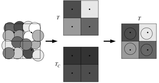
Once again, assuming the particles cover the domain D for all time, we can rewrite the sum as an integral and replace the intrinsic intensity a by a time-varying texture T:

( )

t =

_∫∫

(

−

( )

)

a

( )

s dsd ≅

_∫

T

(

( )

t

)

( )

s ds I x, δ x 1ˆ_ts y tκ y 1ˆ_ts x , κ D y , (4-6)

( )

0,0 i p

( )

t i 0, p

( )

s t i , p

( )

(

p_i 0,0

)



( )

(

_i t

)

t p 0, 1

( )

t d

( )

t fˆ Figure 4-3: (s,t) parameterization of a particle’s position via advection

where the index i has been replaced via the mapping

( )

1

( )

x p

y= _i 0,t = ˆ_ts , (4-7)

and the direction of the integral has been reversed.

The above derivation introduced a time-varying texture T

( )

x,t that represents the intrinsic intensities of the particles as they move over time. Once we have such a texture at a particular time, the standard LIC algorithm will yield the output image for that time:

( )

t =

_∫

T

(

( )

t

)

( )

s ds

I x, 1ˆ_ts x, κ (4-8)

Thus, the basic idea of the algorithm is to first evolve the particles via d to their locations at a particular time, then generate a texture representing those particles, and finally compute the output intensities I

( )

x,t (and O

( )

x,t ) using the texture and vector field f. This process is illustrated in Figure 4-4, and the result is an image representing the field at that particular time that evolves naturally from the previous frame. After an image is rendered, the current time is incremented by a small amount dt and the process is repeated for the next frame of the sequence.

4.2.2 T

EMPORAL

C

ORRELATION

From a visualization standpoint, we would like the intensity of a point on a streamline at a certain time to remain highly correlated with itself as the point moves via d over time. Comparing the intensity of a point as it moves over a small time delta dt:

( )

(

t+dt

)

−I

( )

t =

_∫

T

(

₊′

(

( )

)

t+dt

)

( )

s′ ds′−

_∫

T

(

( )

t

)

( )

s ds

I _tdt x, x, 1ˆ_ts_{dt t}dt x , κ 1ˆ_ts x , κ (4-9) Now, since each point on the streamline at time t moves to another point on the streamline at time

dt

t+ via d, we can come up with a function u

( )

s =s′ mapping these points, as illustrated in Figure 4-5. We can then rewrite the first integral as:

f (Fast) Line Integral Convolution Texture G e n e r a t i o n T I , O Particle A d v e c t i o n a n d A d j u s t m e n t d particles

( )

(

)

(

)

( )

_∫

(

( )

(

_{( )}

)

)

_{( )}

_{( )}

∫

+′ + ′ ′= ₊ + ds ds du s u dt t T s d s dt t T 1ˆ_ts_{dt t}dt x , κ 1ˆ_tu_dts _tdt x , κ (4-10)

Since the particles do not change their intrinsic intensity, we assert that the texture is the same at corresponding points in time:

( )

(

_{( )}

)

(

t dt

)

T

(

( )

t

)

T 1ˆ_tu_+dts _tdt x , + = 1ˆ_ts x , (4-11) This allows us to combine the two integrals:

( )

(

+

)

−

( )

=

_∫

(

( )

)

_

( )

−

( )

s _ds ds du u t T t I dt t I _tdt x , x, 1ˆ_ts x , κ κ (4-12)

Because the relationship between s and s′ may be incredibly complex, this result may not seem very useful. However, consider what happens if we had a well-behaved relationship with a simple convolution kernel:

( )

( ) (

µ

)

µ κ + = ⇒ + =     _{− < <} = 1 1 otherwise , 0 , 2 1 ds du s s u S s S S s (4-13)

The mapping function I have chosen is linear, with the required condition u

( )

0 =0, though other functions that are close to u

( )

s =s would yield similar results. The integral can then be simplified to:

( )

(

)

( )

( )

(

)

( ) ( )

( )

(

)

( )

( )

(

)

( )         + − = − +

∫

∫

∫

+ + − − + + − S S s t S S s t S S s t dt t ds t T ds t T S ds t T S t I dt t I µ µ µ µ µ 1 1 1 1 , ˆ , ˆ 2 1 , ˆ 2 , , x 1 x 1 x 1 x x  (4-14) x

( )

x dt t 1 s s2 s3 _s4 5 s 1 s′

( )

2 2 u s s′ = 3 s′ 4 s′ 5 s′

Figure 4-5: Temporal arc-length parameter mapping

In other words, for a small “stretching” parameter µ, the first term of the difference is approximately µ times smaller than the intensity I

( )

x,t , and the remaining two terms are small corrections at the ends of the streamline.

Qualitatively, when

(

du ds−1

)

is small and κ

( )

s is smooth, the difference in intensity of a particular point on a streamline as it evolves over time will also be small. Thus, we can recognize how points on a streamline move over time by their intensity correlation. In fact, since different points along a streamline are themselves close in intensity, the entire streamline is highly correlated as its points evolve over time.

4.2.3 T

EXTURE

G

ENERATION

If the output image has a pixel size of x∆ , then by Nyquist’s sampling theorem we know that the maximum frequency it can exhibit is 12∆x. Since spatial convolutions are equivalent to multiplication in the frequency domain, and the output image O

( )

x₀ is computed from the texture T

( )

x via the convolution kernels κ

( )

s and χ

( )

x , the frequencies present in O are only as high as the lowest of the frequency extents of T, κ, and χ. Therefore, if the maximum frequency in T is ω<12∆x, then O will also have a frequency extent limited to ω . On the other hand, additional detail in the input texture beyond a frequency of 12∆x is clearly lost in the output. Therefore, we could reduce the frequency extent of T and still achieve similar results in the output O. This is wonderful from an implementation standpoint, since it would have been difficult to work with a function T that had an arbitrary frequency extent.

Returning to the model of discrete particles, we can realistically only work with a finite number. Unfortunately, a finite number of particles represented by delta functions will no longer fill the texture domain. Instead, we let the particles contribute to the texture via a shape distribution function A

( )

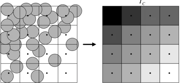
x . The output texture can then be written as a convolution over the sum of particle distribution functions scaled by their intrinsic intensity:

( )

_{∫∫ ∑}

(

( )

) ( )

′ ′         − + ′ = x x p x x x t a A t d T i i i χ , (4-15)

This process is depicted in Figure 4-6. Since the particles are typically very small, their actual shape does not significantly affect the result of the output image. Similarly, the particulars of the convolution kernel are not critical. Thus, for simplicity, in my implementation I choose a square shape function and kernel:

( )

( ) ( )

    ₋∆ _{< <} ∆ ₋∆ _{< <}∆ ∆ =     ₋∆ _{< <}∆ ₋∆ _{< <}∆ = otherwise , 0 2 2 and 2 2 , 1 otherwise , 0 2 2 and 2 2 , 1 2 1 2 2 1 x x x x x x x x x x x x x A x x χ (4-16)

The above integral then simplifies tremendously:

( )

(

( )

)

(

( )

)

( )

   − ∆ <∆ = − − =

∑

otherwise , 0 , 1 , x x x x x u t p y u t p x u a t T i iy ix i x (4-17)

To compute T

( )

x on the pixel grid, for each particle we compute the bilinear interpolation coefficients of its four surrounding pixels, scale by the particle’s intrinsic intensity, and accumulate the results in the four pixels.

Although it is clear that the particle shapes need to mostly cover the texture domain D, it is not as obvious how densely packed they should be. If the particles are separated by a distance roughly equal to the pixel size x∆ , then the maximum frequencies in the texture T

( )

x would be on the order of 12∆x, the frequency cut-off of the output image O

( )

x₀ . If the particle density was greater, then the frequencies in the texture would also be greater, but this could not improve the level of detail in the output image. On the other hand, if the particles were separated by much more than x∆ , we would see a degradation in the output detail. Therefore, distributing particles

T