Dynamic file allocation in a computer network

DYNAMIC FILE ALLOCATION IN A COMPUTER NETWORK

by

Francisco de As's Ros Peran

This report is based on the unaltered thesis of Francisco de Asfs Ros Peran, submitted in partial fulfillment of the requirements for the degree of Master of Science at the Massachusetts Institute of Technology in June, 1976. This research was conducted at the Decision and Control Sciencs Group of the M.I.T. Electronic Systems Laboratory with partial support provided-under ARPA Contract N00014-76-C-1183.

Electronic Systems Laboratory

Department of Electrical Engineering and Computer Science Massachusetts Institute of Technology

Francisco de Asis Ros Perdn Ingeniero de Telecomunicaci6n Universidad Politecnica de Madrid

1972

SUBMITTED IN PARTIAL FULFILLMENT OF THE REQUIREMENTS FOR THE DEGREE OF

MASTER OF SCIENCE at the

MASSACHUSETTS INSTITUTE OF TECHNOLOGY

May, 1976

Signature of Author. .. ... Department of Electrical Engineering and Computer Science, May 7, 1976

Certified by ...

Thes Supervis r

Accepted by ... Chairman, Departmental Committee on Graduate

Students

by

Francisco de As-s Ros Peran

Submitted to the Department of Electrical Engineering and Computer Sciences on May 7, 1976 in partial fulfillment of the requirements for the Degree of Master of Science.

ABSTRACT

One of the main reasons computer networks are a major area of great attention and development today is their ca--pability to provide the facilities for common use of data bases and information files by all computers in the system.

When a file is used by several computers in the network, it can be stored in the memory of at least one of them and can be accessed by the other computers via the communication channels. In ceneral the cost or querying is reduced as we increase the number of copies in the system. On the other hand, storage costs, limitations on the size of the

memories and the cost of updating (every copy must be updated) will dictate decreasing of the number of copies. Further-more if the parameters of the system are time-varying, or if the exact pattern of the rates of demand is unknown or some non negligible possibility of node or link failures is

expected, then some kind of dynamic approach must be used. This thesis considers the problem of optimal dynamic file allocation when more than one copy is allowed to exist in the system at any given time. A general model to handle this problem including updating traffic and the possibility of node failures will be developed. The evolution of the system is represented as a finite state Markov process and Dynamic programming will be used for the solution of the optimization problem.

The use of two types of control variables, one for adding new copies to the system and the other for erasing copies, gives the model certain properties that permit the construction of an efficient algorithm to solve the optimi-zation problem. Within the framework of the developed

model the addition of the updating traffic and the possibi-lity of node failures present no important difficulties. Furthermore the model can easily handle the problem of cons-traints in the maximum or minimum number of copies. In the last chapter the model and algorithms are applied to several numerical examples.

Thesis Supervisor: Adrian Segall

Title: Assistant Professor of Electrical Engineering and Computer Science

ACKNOWLEDGEMENTS

Thanks are due to Prof. Segall who was the original source of this thesis topic and many of the ideas here exposed. Rafael Andreu was very helpful in the computer programming part of the work due to his considerable

experience in this area. Ram6n Bueno contributed with his bilingual ability to the final English structure of some parts of the text. And finally Camille Flores' typing skills permitted to meet the deadline.

This work has been supported by a fellowship from

the Fundaci6n del Instituto Tecnol6gico para Postgraduados, Madrid (Spain) and by the Advanced Research Project Agency of the Department of Defense (monitored by ONR) under

Acknowledgements 3

T_{able of Contents 4}

Lists of Figures 6

CHAPTER I.- INTRODUCTION 8

I.1.- General Setting and Description 8

of the Problem

1.2.- Summary of Results 14

1.3.- Chapter Outline 15

CHAPTETR II.- DESCRIPTION OF THE MODEL 17

1.].-- Characteristics, Basic Assumptions

and Operation Procedure 17

1I.2.- Data, Parameters and Variables 20

II.3.- Objective Function 22

11.4.- Control Variables and Restatement

of the Objective Function 22

II.5.- Definition of State and Dynamics

of the System' 25

II.6.- Some Useful Properties of the Model 29 CHAPTER III.- DYNAMIC PROGRAMMING AND BACKWARD

EQUATIONS 35

III.1.- Preliminary Remarks 35

III.2.- Backwards Recursive Equations 36

III.3.- Recursive Equations for NC=2 38

II'I.4.- Recursive Equations for NC=3 and

III5.- Constraints in the State Space 56 CHAPTER IV.- UPDATING TRAFFIC AND NODE FAILURES 59

IV.1.- Updating Traffic 59

IV.2.- Network with Node Failures 62 IV.3.- _{Recursive Equations for NC=2}

con-sidering Node Failures ₆₅

IV.4.- _{Recursive Equations for NC=3 and}

a General NC considering node Failures 71 CHAPTER V.- _{NUMERICAL APPLICATIONS AND OTHER}

ANALYTICAL RESULTS 93

V.1.- Time Varying Rates. No Failures.

No Updating Traffic ₉₃

V.2.- Constant Rates. Updating Traffic.

No Failures ₉₈

V.3.- Nonzero Failure Probability 123 V.4.- _{Completely Simmetric Network 136}

CONCLUSIONS AND OPEN QUESTIONS ₁₄₀

APPENDIX A _14.6

APPENDIX B ₁₄₈

APPENDIX C ₁₅₀

LIST OF FIGURES

Fig. Number Page

1.1.- General representation of a computer

network reflecting the problem of

file allocation. 10

II.1.- Illustration of the Operation Procedure. 19

II.2.- Sequence of events at any time t. 28

II,3,- Transition tableau for the case NC=2

(assuming deterministic transitions). 31

II.4.- Transition tableau for the case NC=3

(assuming deterministic transitions). 32

11.5.- Flow graph showing the steps to obtain

the transition tableaus. 34

III.1,- How to obtain the first row of the

transition matrix from the first tableau

row. 39

Ii.2.- Flow-chart showing how to obtain the

per-unit-time cost vector. 43

III.3a).- Flow-chart showing how to construct the nonzero probabilities of row n when

the decision is "go to state m". 51

III.3b).- Fortran flow-chart of Fig. III.3a). 52

III'4.- Flow-chart of the optimization process. 54

IV,1.- Sequence of events including updating

traffic. 60

IV.2,- Flow-chart of updating traffic when

failures in the computer are considered. 73 IV.3,- Flow-chart showing how to obtain terminal

and per-unit-time costs. 74

IV.4.- Tableau of possible transitions for NC=3. 76

IV,5,- Flow-chart showing how to obtain the

transition matrix and the optimal decision

for a netrowk with failures, 81

IV.6.- Optimization process for a network with

failures. 89

IV,7,- Reordered transition tableau showing

Fig, Number Page

V.1.- Rates, Case 1, 96

V.2.- Cost curves for static and dynamic

approximation. 97

V.3.- Rates. Case 2. 96

V.4,- Qualitative sketch of a typical behavior for a system with constant parameters. K is the optimal set and Kc its com-plementary (only some states are

repre-sented). 105

V.5.- Optimal transitions for the example of

section V.2 with P=0.25, C -0.25. 106

V.6.- Total cost vs. storage cost with p as a

parameter. 112

V.7,- Total cost vs. p with Cs as a parameter. 113 V.8a).- Total cost vs. storage cost with p as

a parameter. i represents trapping

state and j optimum initial state. 124

I-1 General Setting and Description of the Problem "The time sharing industry dominated the sixties and it appears that computer networks will play a similar role in the seventies. The need has now arisen for many of these time-shared systems to share each others! resources by coupling them together over a communication network

thereby creating a computer network" (L. Kleinrock[l]). We define a computer network to be an interconnected group of independent computer systems communicating ,with each other and .sharing resources such as programs, data, hardware, and software.

The increasing interest in this area is the cause for a continuously .growing number of articles, books and projects related to computer networks [2.1 -[7], [24]. The reasons why these types of networks are attractive are widely exposed throughout the literature in this field.

a) sharing of data base, hardware resources, program and load

b) remote data processing

c) accessto specialized resources

d) recovery of informationfrom a remote node in case of node: failure

-~~l----e) decentralization of operations and need to trans-fer information from one point to another etc. One of the main reasons computer networks are a major area of great attention and development today is their

capability to provide the facilities for common use of data bases and information files by all computers in the system. This work deals with the problem of the information

alloca-tion to be shared by the computers in the network. Such a network is displayed in Fig. 1

When a file is used by several computers in the network, it can be stored in the memory of (at least) one of them

and can be accessed by the other computers via the communi-cation channels. In general, the cost of quefying is

reduced as we increase the number of copies in the system. On the other hand, storage costs, limitations on the size of the memories and the cost of updating (every copy

must be updated) will dictate decreasing of the number of copies.

The problem of how many copies of the files are to be kept and their allocation is the main subject of this Thesis.

Most of the previous work in the area of file alloca-tion has been devoted to the analysis of the problem under static approximations, that is, assuming that all parameters of the system are known a priori and basing the design on their average value over the period of operation of the system. The location of the files is then considered fixed

MEMORY

CO U\ -,COMPUTER

T

MEMORY

_OOMPUTER 3

~c~

~\

MEMORY SMEMORY FILES

LA

I

How many copies of each file do we need in the network?

At which computer do we have to allocate each copy?

For how long must a certain alio-cation distribution remain unchangeable?

etc.

-Fig. I,:'. Ge-neral representation of a computer network reflecting the problem of file allocation

The criterion of optimality used in C81, is minimal overall operating costs. The model considers storage and transmis-sion costs, request and updating of the files and a limit on the storage capacity of each computer. The model

searches for the minimum of a non-linear zero-one cost

equation which can be reduced to a linear zero-one program-ming problem.

Another work is a paper by Casey

L91.

He considers a mathematical model of an information network of n nodes, some

of which contain copies of a given data file. Using a

simple linear cost model for the network, several properties of the optimal assignment of copies of the file are demons-trated. One set of results expresses bounds on the number of copies of the file that should be included in the net-work, as a function of the relative volume of query and update traffic. The paper also derives a test useful in determining the optimum configuration.

Of very recent appearance is a paper by Mahmoud.and Riordon

[22]

. In this paper the problems of file allocation and capacity assignment in a fixed topology distributed

computer network are simultaneously examined. The objective, in that analysis, is to allocate copies of information files to network nodes and capacities to network links so that a

-~~~~~~~~~~~~~~~~~~~~~~~~~~~~~~~~~~~~~~~~~---minimum cost is achieved subject to network delay and file availability constraints. The deterministic solution for a medium size problem is intractable due to the large amount

of computation so that an heuristic algorithm is proposed. A quite different analysis in which the important

quantity to be optimized is the service time, instead of the operating cost, is done by Belokrinitskaya et all.

[10].

The analysis results in a zero-one nonlinear programming problem (that can be linearized), similar to the one in [8j.

In the above mentioned works, the-problem is considered under static conditions and using average values of the

parameters.

If the parameters of the system are time-varying, however, or if the exact pattern of the rates of demand is unknown or some non negligible possibility of node or link failures is expected, then some kind of dynamic approach must be used.

It has been only recently that the first studies of these problems, from the dynamic point of view, have begun to appear. In a work by A. Segall

11]

the problem of finding optimal policies. for dynamical allocation of files in a computer network that works under time-varying opera-ting conditions is studied. The problem is considered

under the assumption that the system keeps one copy of each file at any given time. The case when the rates of demand

are not perfectly known in advance is also treated. Only a prior distribution and a statistical behaviour are assumed, and the rates have to be estimated on-line from the incoming requests.

The problem of optimally allocating limited resources, among competing processes, using a dynamic programming

approach is studied in 12]. A dynamic programming approach is also suggested for the problem of minimizing the costs of data storage and accesses in [25]. Here two different types of accessing costs are considered. The accessing cost will depend on whether a record is to be read or to be written

(migration). _{A different approach to the same problem is} taken in [2J . A two-node network with unknown access probabilities is considered. The problem is to set up a

sequential test which determines the earliest moment at which migration leads to a lower expected cost.

The present work considers the problem of optimal

dynamic file allocation when more than one copy are allowed to exist in the system at any given time. A general

model to handle this problem including updating traffic and the possibility of node failures will be developed.

The evolution of the system is represented as a finite-state Markov process and dynamic programming will be used for the solution of the optimization problem.

1.2. Summary of Results

A model for the analysis of optimal dynamic file allo-cation is introduced, The use of two types of 'control variables, one for adding new copies to the system and the other for erasing copies, gives to the model certain proper-ties that permit the construction of an efficient and rela-tively simple algorithm to solve the optimization problem. Among others, the algorithm is efficient due to the fact that

it computes only the nonzero transition probabilities. A detailed set of flow-charts and Fortran program listings are given for all. the operations and calculations that take place in the optimization process.

Within the same framework the incorporation of node failures presents no important difficulties, except for increasing the number of states. Some kind of constraints in the state space, those that could be represented as

reductions in the set of admissible states, are also easily handled by the model.

In the last chapter we apply the algorithms to several numerical examples. For the case of constant rates of demand with no failures in the computers the corresponding Markov processes have a trapping state. For these processes it will be shown that the general dynamic programming algorithm

need not be implemented, and a much quicker answer. to the optimization process can be found.

For the more general case of constant parameters with possibility of node failures included,. quick convergence to

the steady state optimal dynamic decision policy was found for all examples.

Finally it will be shown that having a completely

simmetric network (equal parameter values for all computers and links) will allow a considerable reduction in the number of states.

A more detailed exposure of results can also be found in the chapter dedicated to "Conclusions and Open Questions".

I.3. Chapter Outline

In chapter II we begin with the description of the model. We first state the general hypothesis and basic assumptions to be considered throughout the study and continue with the description of the operation procedure. We indicate the objective function and define the control and allocation variables. The chapter ends with the definition of the state and the description of the dynamic equations of the system.

In chapter III Stochastic dynamic programming is applied to the model to determine the optimal allocation strategy. First we will write the recursive equations for a simple net-work with only two computers and then we will see how easily

these equations generalize to any number of computers. We finish the chapter indicating how the model can handle the problem of certain constraints in the state space.

framework with the inclusion of the updating traffic and the possibility of node failures. As in chapter III, we first write the recursive equations for a network with two computers

and then generalize them to any number of computers. At

this point we give a very detailed set of flow-charts, showing how to compute the different matrices and vectors of the

recursive equations and how to carry out the whole optimi-zation process.

Chapter V deals with numerical applications. Using the insight gained from numerical answers some additional analytical results are developed.

A few pages dedicated to general conclusions and further work to be done in this area will follow this chapter.

Two appendices, A and B, expanding results of chapters II and III will also be added. A third appendix contains a set of Fortran program listings corresponding to the most significant flow-charts of previous chapters, These programs have been used to implement the numerical applications of chapters V. Auxiliary subroutines are also listed.

CHAPTER II

DESCRIPTION OF THE MODEL

II.1 Characteristics, Basic Assumptions and Operation Procedure

We shall make here several simplifying assumptions, that are still consistent however with the models appearing in real networks. _{We shall assume that the files are} reques-ted by the computers according to mutually independent

processes (with statistics to be specified presently) and also that the files are sufficiently short. Moreover the communication lines are taken to have sufficient capacity and the computers sufficient memory, so that the transmission of the file takes a very short time and there is no

res-triction on how many files a computer can carry. Under these assumptions, it is clear that in fact the files do not interfere with each other, and we can therefore treat each file separately.

The analysis will be done in discrete time, assuming the existence of a central synchronizing clock. It will be considered that with previous assumptions the time interval between clock impulses is long enough to allow the execution of all the necessary operations to take place in it (request arrivals, "reading" of present state, implementation of

Chapter IV.

We' _{may .summarize the assumptions as follows:}

1) No failures in'the network (relaxed in Chapter IV) 2) Channels with sufficient capacity (or sufficiently

short files)

3) Sufficiently large storage capacity at each computer 4) Requesting according to mutually independent processes 5) Files are treated separately (according to former

assumptions the files do not interfere with each other)

6) The analysis is done in discrete time

The proposed:procedure is similar to that proposed in reference [11], with the only difference being that we now allow more than one copy at each instant of time (the way the updating traffic is taken in consideration will be described in Chapter IV).

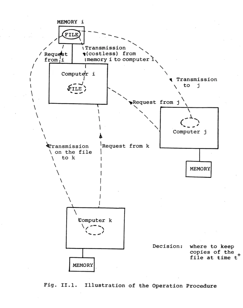
The.procedure is illustrated in Fig. II.1 and can be described as follows: _{Suppose a certain number of copies is} stored at time t in the memories of a set of computers,

say I. If at-time t the..file _{.is requested only-by computers} in the set I then no transmission cost ..is incurred and.a decizsion has to::be made,whether to erase some of the copies from I (with the specification of the particular copies to

MEMORY i

/ I

%Transmission

/ Requekt

i(costless) from

from i

Imemory i to computer

1\

I

'

.

\

Computelr i

.

I

~ Transmission

to j

ILE

E

VRequest from j

Computer j

Trransmission

IRequest from k

on the file

I

to k

MEMORY

Computer k

Decision: where to keep

copies of the +

file at time t

MEMORY

be erased) or to keep the same number of copies. If, on

the other hand, the file is also requested by other computers not in-I, then the file is transmitted for use to these

computers and a new collection of copies, say J, appears in the system at time t+ _.

A similar decision now has to be made but with the set J instead of the set I

The restriction of reallocating the file only in conjunction with a regular transmission is reasonable for this model, because if a change of location is decided upon, one might as well wait until the file is requested for the next time by the appropriate computer, otherwise it is conceivable that the file might be transferred back and forth, without anybody actually using it.

II.2 Data, Parameters and Variables

In this section part of the notation used in the study will be introduced.

Consider a completely connected network of NC computers. The requests of the file by the computer will be modeled

as mutually independent Bernoulli processes with rates e (:t'), i = 1,...NC, that is

Pr{ni(t) =

l}

= 1 -

Pr

{ni(t)

0

0 = =ei(t) (2.1)

where ni(t) = 1 indicates that the file has been requested by computer i at time t. The rates 8i(t) are assumed to be known for 'all computers and instants of time.

We define the variables

1 if there is a copy stored at computer i at

Yi(t) = time t (2.2)

Otherwise

i

= 1,..MC

The condition of having at least one copy of the file in the system at any instant of time can be analytically expressed as

NC

E Yi (t) > 1 VtC [OT (2.3)

i=1

where T is the whole period of operation. The operation costs are

C_i = storage cost per unit time per copy at memory i

Cij = communication cost per transmission from computer i to computer j

i, j = 1,... NC i ~ j

We will assume C.. = O Vi 11

It is assumed that these costs are time-invariant; the case with time-varying costs can be handled by simply writing Ci(t) and Cij(t) throughout the paper.

II,. 3 O'bjiective .Funct.io-n

.Supposi£ng thatt the user access.es that copy of the file that- minimizes his communication .cost ..and., denoting -si- 'i-bol.ical'ly'.by I(t) the :set of nodes :having a copy at 'time t, we 'can write t.he expression for the total expected cost over the :period [O.,T] as

'T NC NC

C. =E Ci:yi(t)+ (-l-Yi (t))n.(t)min Ci _(2.4)

t-'O i=l i=.l k-eI (t)

The first sum in the bracket represents the total storage cost at time t and t-he second sum is the total transmission cost. _{We can see that summands contributing to the} trans-mission cost are those with yi.(t) = 0 and ni(t) = 1 only, that

is, those coming 'from computers 'that do not have the- file and have had a request.

The goal 'is to design a closed-loop control that.will dynamically as:sign the loca'tion of the fil-e and .will .minimize the defin-ed expected cost. We introduce the control'variables in -the -next section.

II.4 .Control Variables and Restatement of the -Objective : Fun.c-t ion

We-will- define two types of control variables. One will' .correspond _{.to the era.sure process and the other one to the}

in two types of control variables will simplify significantly the amount of notation.

The variables are

1

f

if the decision is to erase the copy from i at time t assuming the copy was there at

Ci't3=l Sat time t (i.e. Yi(t) = 1) (2.5)

0 - otherwise

1 - if the decision is to keep a copy in i at time t+ assuming that the copy was not there ai(t ) = ' (yi(t)=O) and there was a request from that

computer (ni(t) = 1) (2.6)

O - otherwise

i = 1,..NC

These definitions require the introduction of the con-cept of active control variables. It will be said that the variable ci(t) is active if Yi(t) = 1 and that ai(t) is active if Yi(t) = 0. Due to these definitions ai(t) and

Ei(t) _{cannot be simultaneously active. From definitions} (2.5) and (2.6) the nonactive variables will always be equal zero. Therefore only active variables will be con-sidered throughout the analysis.

With the previous notations, the dynamic evolution of the system is:

a) Yi(t+l)= y (t)t)[l-Ei ] + [1-Yi(t)ai(t)ii (t )

i = 1,L,..NC (2.10a)

NC

iff E (right hand side) / 0 i=l

b) yi(t+l) = yiTt) i = 1,2,..NC (2.10b)

NC

iff (right hand side of :(2.10a)) = 0

i=l

Equation i(2.10b) shows that if our decision variables are such that all copies of the file will be erased, then no decision variable is actually implemented, and there-fore the system remains in the previous state. Otherwise, the -system evolves according to equation (2.10a) namely computer i will have a copy at time (t+l) if

i) it had a copy at time t (Yi(t) = 1) and the decision was not to erase it (c_i(t) = 0) or

-ii) it did'not have a copy at time t and therewa.s a reque.st from-computer i (n.(t) = 1) and a decision to write the

1.

file into memory i was taken (ai(t) = 1).

-The optimization problem could then be stated .as follows: 'Given the zdynamics (2.10), find the optimal control policies

s~(t) I i = 1,1,..,NC at(t) t 1,2,..T

and the initial locations Yi(O), Vi, so as to minimize the expected cost (2.4).

Hence we have a dynamic system in which the inputs are a sequence of decisions made at various stages of the evolu-tion of the process, with the purpose of minimizing a cost. These processes are sometimes called multi-stage decision

processes

[151.

II.5 Definition of State and Dynamics of the System

Being at a certain instant of time, in the optimization process, the only information needed, given the fact that the request rates are perfectly known, is the identification of the computers that have a copy of the- file at that time. With only this information we can continue the optimization process and the past is inmaterial as far as the future is concerned. Therefore the location of the copies at any instant of time summarizes the information needed at that instant (together with the rates) and the problem then is to find an optimal policy for the remaining stages in time.

The state of the system will be defined, at time t, as the location of the copies of the file at that time and it will be represented by a vector with NC binary components,

having a zero in the places corresponding to computers that do not have the file and a one in the places of computers having a-copy. These vectors will be named by the decimal

number Whose binary representation is the NC- dimensional vector and will be represented by a capital Y.

Therefore the Stat:e at time t Will be the column vector

YlW(t

Y(t) = y2

(t)

(2.11)

.Y2 2(t)

YNC(t) .

or alternatively the state of the system at time t is m(t) where

m(tj = decimal 'number with binary representation given by the sequence Yl(t) Y₂(t)-Y CN (t)

m 1,2, ... ,M NC

M = 2 1

m = 0 will not be a valid state because it corresponds to the case of having no copies in the system and this' situation has to be avoided. Thus the previously stated condition

NC

L 'Yi(t)l>

1

i=l

The dynamics of the state are easily obtained from the dynamics of the allocation variables: we only have to

substitute for each component of the vector defining the state Yl (t) 0 yl(t) Y₂(t+1) 1-E2(t) O y2(t) y c(t+l) O 0 0 0 . , fct)NC(t) al (t )n l ( t ) O . O 02 2~ 01-Y ₁ (t) o a₂(t)n₂(t) * .* 1-y₂(t) 0 (t)n(tl (t) 0 ( NC (t)nNC (t yNC(t) (2.12a)

iff right hand side of (2.12a) O0 and

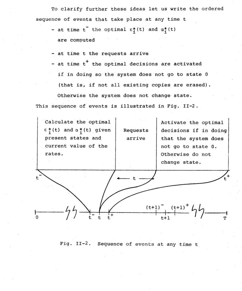
To clarify further these ideas let us write the ordered sequence of events that take place at any time t

- at time t the optimal si(t) and x*(t)

1 1i

are computed

- at time t the requests arrive

- at time t+ the optimal decisions are activated if in doing so the system does not go to state 0

(that is, if not all existing copies are erased). Otherwise the system does not change state.

This sequence of events is illustrated in Fig. II-2.

Calculate the optimal Activate the optimal

· (t) and a*(t) given Requests decisions if in doing

present states and arrive that the system does

current value of the not go to state 0.

rates. Otherwise do not

change state.

t

/--t

.

.

-2

Seq

(t+l)-s

(t+l)a

tim

0 tt t t +l T

II.6 Some Useful Properties of the Model

So far the main structure of the model has been des-cribed. In this section, we describe some of the properties of the model. First of all we will look at the transitions among states.

Recall from section II.4 that the active variables are defined as

Ci(t) is active if Yi(t) = 1 ai(t) is active if Yi(t) = 0

Hence these variables are uniquely determined by the state. For instance, having a network with five computers (NC=5) and being in state eleven (01011) the active variables are

State Y₁ Y₂ Y₃ Y₄ Y₅ active variables

Y= 11 - 0 1 0 1 1l a 2 a 3 4 £5

witha's corresponding to places where there is a 0 (no file in the memory of that computer) and £'s to places where there is a 1 (there is a copy at that computer). The non-active variables will then bel1, c2' £3 , 4 and a5 and we saw, also in section II.4, that their value is equal zero no matter which decision is taken, so we can omit them.

Suppose now that the optimal decision at a given time is: - erase copies from computers 2 and 5

- keep a copy at computer 3 or in terms of the control variables

u = ( c1 E2 C3 c4 C5) = (0 i 1 0 1)

Thus, if there is a request from computer 3, the system will go to state

Yl Y2 Y3 Y4 Y5 _ state 6

-0- 0 1 1 0

and if'-there is no request from computer 3 the system will go to

1 ..2 3 4 5

state 2

0' 0 0 1 O0

Because of the unique correspondence in the notation-we see that it is equivalent to say that the decision is

u1= ( a a34 O1

£

( 1 1)

or-"go to state 6"

For the sake of: simplicity these two' forms will? be interchangeably used.

From the above analysis it can be seen that

(init:ial state) .· (decision vector) = (final desired'- state) (decision vector) = (initial state-)

*

(final desired state) wheere demeans "exclu"sive or". This is so because if a con-trol variable: has a value 1 we: have to change thee value of the allocation variable in the transition, while if the value is 0 there .isno change in the transition. This kind of

operation is.exactly- the "exclusive or" addition.- In

--particular for the example above 11 --- 0 1 0 1 1 + O 1 1 0 1 al 2 3 c4 5 -. 0. 0 1 1 0_

6

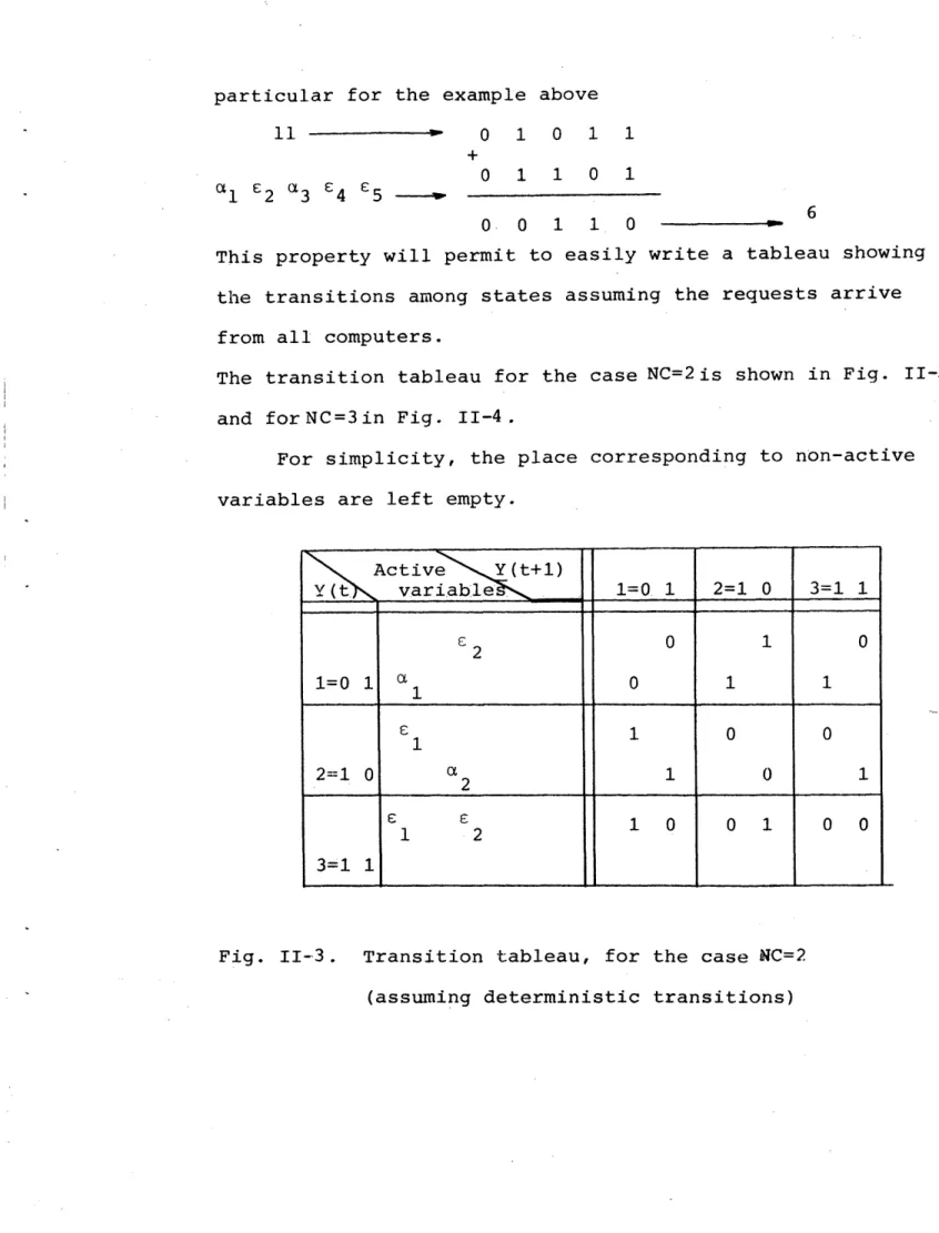
This property will permit to easily write a tableau showing the transitions among states assuming the requests arrive from all computers.

The transition tableau for the case NC=2is shown in Fig. II-3 and forNC=3in Fig. II-4.

For simplicity, the place corresponding to non-active variables are left empty.

Active .(t+1 ) Y(tsK variab~le 1=0. 1 2=1 0 3=1 1 -c 0 1 0 1=0 1 1 0 1 1 1 1 0 0 2=1 0 2 1 0 1 1 2 1 0 0 1 0 0 3=1 1

Fig. II-3. Transition tableau, for the case NC=2 (assuming deterministic transitions)

V-i ) ri · i ,-4 -4 0 C l/4 H H

~0

0 r-li r-q C> OC C "t-I

~~i~~~~~~~

rC ,--I 0 0... ,..4 0 C) 4J~~~~~~~~~~~~~~U O r a 0-0 .'H ... : OI ' O C) C. '

~ ~

-. H 0 0 - 0 O H . q ll 3 ., . .. ---.--- - , C) rt~~~~~~~~~~~~~~~~~~~~~4~~~~= 0 . , HIi~~~~~- H-- 00 0 , -- 0

o

0 ,-I o 0 0 4J ' -I 0 --

t

_{~~~~~~~~~~~~~~~~~~~~t}

0 0 0 E na ,..4 o q/' o H 0 H 0 0 , o0" 0 H~~~~~~~ II~~ H (H 0 0

].

,"' :" *'l' " ~ '. II r

~~~~~~~~~~~0

_C)) C) 44~~~~~~~~~~~~~~~C ' _{v-I 0} 0 H . --H i~~~~~~~~~,-4 0,--I 0~~~~~~~~~~~~~~~~ 'I(%J~T-

a:r

HO 001 1 0 H 0 H 0 o~~ Hd

~~o

0 0 H H .~. ,- UI co co co oo oqc o

tiU~~~~~e

oi e,, t', eqol

.,-, l .

~~~.s

~

t w ~3 ~ w c0 'l [ rl~~~~~~~~~~~~~~~~~~~~~~~~~~~~~~~~~~~~~~~~. I "i -I ,.o ). -.i _

~~~~~~~~~~~~~

II " -~1I

~~~~~~~~~~~~~~~~~~~,,

>.~~

~

(Y ) U)

These tableaus will prove later to be of great utility for the construction of the transition probabilities among states. As we said before, we can write this tableau

mechanically and this is important in computer calculations. Summarizing, for a network with NC computers, the steps are the following:

1 - If the system is in state m, write m in base 2 with NC digits.

2 - Assign a control variable a to the places where the digit is 0 and a variable £ to the places

where the digit is 1.

3 - To obtain the value of these control variables in a transition from m to n, compute m @ n, where n

is also written in base 2 with NC digits, and assign the values of the resulting digits to the corresponding control variables.

4 - To obtain the mth row of the tableau repeat step 3 NC

for values of n from 1 to M (M = 2 -1)

5 - To obtain all the rows of the tableau repeat from step 1 for values of m from 1 to M.

The flow-chart corresponding to these five steps is shown in fig. II-5.

Repeat from m = 1 to M to obtain

all the rows of the tableau

Write m in base 2 with NC digits

and call the digits mi

if m. 0 the ith control variable

"is ti

if m. = 1 the ith control variable

is cE:

i

i = 1,..NC

Call u. to the ith variable (ai

or c

_i)

Repeat from n = 1 to M

_

to obtain all the elements of row m4,

Transition to state n:

write n in base 2 with NC digits

Compute m e n = k, k_i ith digit u. = ki i = 1,..NC

Fig. II-5.

_{Flow graph showing the steps to obtain the}

CHFAPTER III

DYNAMIC PROGRAMMING AND BACKWARD EQUATIONS

III.1 Preliminary Remarks

It can be easily seen that the model described in chapter II has all the properties needed for the application of

dynamic programming, [13] - [16]

In particular it is obvious that the separation property holds for the cost function, eq. (2.4). The MTarkovian state property is also satisfied, see section II.5. Hence the problem is:

Given the dynamic equations (2.12), find the optimal dynamic allocation strategy, using dynamic programming, to minimize the cost (2.4).

We will separate the total expected cost (2.4) in two parts

T-1

C = E {H [Y(T)]} + E E L[Y(T),T] (3.1)

f =0

where NC NC

L[Y(T),T] = Ciy_i(T) + (1-y 1(T))ni (T) min Cki (3.2)

keI(T)

i=l i=l

is the per unit time, or immediate, cost, and

H CY(T)h = L [Y(T),T- (3.c3)

The cost to go at time t given that the system is in state i will be defined as

T

Vi(t) = E E L[Y(T),r]

1Y(t)

= i I (3.4)

t=t

and the optimal cost-to-go

V*(t) = min V.(t) i = 1,2,..M (3.5)

1i u(t) 1

From the Markovian property, the following equalities can be easily proved, see ref t11].

E {L

[Y(T),T] IY(t),

t

=,1,..}-E {L CY(),~Y()1T} = (3.6)

NC NC

CiY i (T- _{+ , E~~} (T. E)-) i (T) _kekI() min _(T Cki (T

i=l.i=l

III.2 Backwards Recursive Equations

The backwards equations for this probabilistic system can be written (see [11 pag 955)as

NC

V*(t)=min{E{L[Y(t),t] IY(t)=i} + Pij(t"u)V* (t+1) (3.7)

j=l

i = 1,2,..M

where Pij (t,u) is defined as the probability of being in

is in state i at time t, that is,

Pij(t,u) = Prob {Y(t+l) = j

IY(t)

= i,u(t)} (3.8)

From the expression (3.2) of the per unit time cost at time t observe that the decision u(t) at time t affects only the state Y(t+l) at (t+1) but not Y(t) and n(t) and therefore the immediate L(t) cost is control independent.

If u* is the optimal control and V* the corresponding cost to go, then:

NC

VI(g)=E {L [Y(t),t] 'Y(t) =i} + Pij(t,u)V(t+) (3.9)

j=l i = 1,2,..M or in vector form

V*(t) = A(t) + P(t,u*) V*(t+l) (3.10)

With this notation it is clear that the total minimum expec-ted cost over the period [0O,T1 will be the smallest component of the vector V*(0O) and, the state corresponding to this

component will be the optimal initial state.

To pursue further with the investigation of the actual form of the vector A(t) and matrix P(t,u*) we will begin with the cases NC=2 and NC=3, the generalization to a larger

III.3 Recursive Equation for NC=2

For the case of two computers the expression of the total expected cost over the period

OPT]

can be written as

T 2 2

C=E C _Yi(t) i E (1-Yi(t))ni(t)C_k t

t=O i=l . .i=l k/i

= E [ ClyYl(t)+C2Y2(t)+(l-Yl(t) )1(t)C21+(1-Y2(t))82(t)C12] t=O

twO - (3.11)

where we have applied (3.6) and the condition that yl(t)

+ Y₂(t) > 1. Therefore

L[Y(t), t] =ClYl(t)+CY2 2(t)+ (l-yl(t))l1(t)C2 1+(l-y2 (+))e 2(t)C12 (3.12) From this expression we obtain immediately the components of the vector A(t)

Xl(t)=E{L[Y(t) ,t]

IY(t)=(O

1) =1} = C2+C 21 l (t)

A2(t)=E{L [Y (t) ,t] Y(t)=(1 0) =2} = C1+C1 282(t) (3.13)

3(t)=E{L[Y (t) ,t] Y(t)=(1 1) =3} = C+C

To obtain the elements of the probability matrix it is very important to follow carefully all the conditions, see Fig. II-.2, imposed on the decision process. Following those rules we have obtained in Appendix A the elements of the transition matrix, as

1-a(t)el(t)

Ec(t)

al (t)8l(t) (1-E

(t))e~

(t)el(t)

P(t,u*) c*( (t)e(t)8₂(t) 1-c*(t)8₂(t) (1-6*(t))ac(t)8₂(t) (3.14

M1(t), *M (1-6 (t)) C*(1-6()(t) (1-(t)) (1-C*(t))

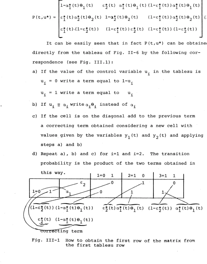
It can be easily seen that in fact P(t,u*) can be obtained directly from the. tableau of Fig. II-6 by the following cor-respondence (see Fig. III.1):

a) If the value of the control variable ui in the tableau is Ui = ° write a term equal to l-u1

u. = 1 write a term equal to ui

b) If ui i write i.ei instead of (i

c) If the cell is on the diagonal add to the previous term a correcting term obtained considering a new cell with values given by the variables yl(t) and y₂(t) and applying steps a) and b)

d) Repeat a), b) and c) for i=l and i=2. The transition probability is the product of the two terms obtained in

this way. 1=0 1 2=1 0 3=1 1

-0 I 1 0

2 /0

1=0

'

-

/

.-

1

(.e£

·

(t))

(1-a

₁ (t )e l (t ))

6

(t)a*

₁ (t )e l (t)

(1-E

_{2 12}

(t)) a*(t)el(t)

E

(t) (1-a (t)e

_l

(t))

rring term

Fig. III-1 How to obtain the first row of the matrix from the first tableau row

This is not a surprising result and it could be easily expected from the way the tableau is constructed. Step C) is a consequence of the condition imposed that if after the arrival of the requests the optimal decision requires to erase the last copy of the system we remain in the same state.

Therefore the probability of remaining in the same state (diagonal terms) has to be corrected by a term equal to the probability of requiring the erasure of the last copy. This probability is exactly the probability of g oing to state .0

if this state were allowed,. The values of the control variables needed to go to state 0 are obtained through the ".exclusive or" addition of the binary representations of present state and -state 0, but this suis sum is always equal to the present state repre.senntation; therefore the valuues of ,the control variaDbl~es .are equal to the vvalues -of the alloca-ti:on variabl:es of the presen~t state.. In -this way we ensure that ithis mattr. ix .accomplishes all the properti-es of a stochastic ;maktrix;, in

particular Ithe needed condi 'tion thvat all rows must add to one; this is so because !the terms are obtained using all ,possible combinations of

O0's

and l'Vs with two elements

(NC

elements in general') and hence we always add terms like

A B+(l-A)B,+A(l-B+(l-A) + ( A(3.15)) (1-B)

Another simplification can be obtained by observing

that in ·every row the combination of rcontrol values that will take the system into the state Y-(t+l)=-0 is -not allowed. Fo-r example in the first row of Fig. 11-3, l=x0 s2=-1 is forbidden

and therefore in the first row of P(t,u) we have

(1-a₁

)E2

= O (3.16a)

Similarly in the second row of P(t,u)

(l-a2)E: = 0 (3.16b)

and in the third row

£1 £2 = 0 (3.16c)

This property will be useful sometime to simplify the expression of the transition probabilities. We have made use of this property in Appendix A.

Grouping all results together we obtain the following backward matrix equation (NC = 2)

V*(t) C2 + C21i(l t)

V*(t) = C + C122(t) +

V*(t) C1 + C 2

1-a* (t Et)1 t(t)et M(t)1 (1-(t) (t)(t) V(t) V(t+)

c1 ( et t) ( t) a* 2 (t) (l-E (t) (t)2(t)(1-(t) 82(t) V(t+l) £1*(t) £2 (t) 1-c* (t) -6(t) V (t+1)

1 2 1 2 3

(3.17) where the optimal decisions for each row of the matrix

P(t,u*) are the values of the corresponding row in the tableau that give minimum scalar product with the vector V*(t + 1)

In particular, if we define A=V (t+1)

B= (1 -9(t))V*(t+1)

+e

(t)V* (t+l) (3.18)

c= (1-e

(t))V*

(t+l)+8

₁

(t)V (t+1)

then if the system is in state i at time t

I

c~(t) = 0if A < B and A < C(3.19a)

Ot tt) =

0

(c2(t) 1 { if B < A and B< C (3.19b) E£2(t) = i

{if

C < A and C < B (3.19c) £*(t) = 0

In the same way the optimal decisions being in state 2 and 3 can be obtained.

We will see some numerical applications of these equa-tions in chapter V.

IIi-4. Recur~sive Equations for NC=3 and Generalization to

any NC

-For NC=3 the total expected cost over the period [0,T] can be expressed as (remember C. = 0, Vi)

11

T 3 3 3

C = E E[Y' EC1Y.(t) E EY yi(t)yi(t)nk(t)minClk

t=l i=l j>i k/i ijt

T

- E L[Y (t),t] _(3.20)

The components of the vector A(t) are obtained as

Al(t)=E {L[Y(t),t] Y(t)=(O 0 1) = 1} = C3+C3 1l(t+C 3 2e2(t)

A2(t)=E {L [Y((t) t]IY(t)=(O 1 0) = 2} = C2+C2 1 1 (t)C 2 (t)

x

₃(t)=E {L[Y(t),t]IY(t)=(O 1 1) = 3} = C₂+C ₃+e8(t)miniC₂1,C₃ 1_t t" " " " " - - etc. (3.21) The whole vector is

C3 + C3 1 l1 ( t ) + C32 82(t) C2 + C21 81(t) + C23 e 3(t) A(t) = C₂ + C₃ + 81(t) min (C_{2 1}, C_{3 1}) (3.22)

C

1

+ C12 e2(t) + C

13

3(t)

C1 + C3 + 8₂(t) min (C1 2, C32) C₁ + C₂ + 83(t) min (C_{1 3}, C2 3) C₁ + C₂ + C₃

The way to construct these components from the state vector is simple.

The easy rules are sketched in the flow chart of Fig. III-2.

Repeat from m=1 to M State m

write m in base 2 with NC components mi ith component i=l,..NC

Fig. III.2 Flow chart

to obtain the per J - set of indexes such that m.=0 unit time cost

vecunit time cost set of indexes such that mi=l

vec(t)o Cs+ uhmin {C.. .

m B r

As far as the probability transition matrix is concerned, we can calculate easily its components by making use of the ~ rules-stated for the case NC=2 and -the tableau of Fig.- II-7.

Some of the components are shown below (for brevity.we delete the variable t).

(1-a (1-el 202) . 21)e2e2)3

(1-e1F)2a383 _(1-a8e1) (1-a33) . .

P(t,u) = (3.23)

1,1e) 1-2 ( 3 ) (1-el ) (1-2£ 2 33

61

2 13

where we have applied a property similar to (3:.16) so that for example in the 7th row of P given in (3.23) we have

l 2:£3 0.

It can be seen now that the rules we developed in cons-tructing the immediate cost vector and the transition pro-bability matrix for NC=2 and NC=3, generalize easily for a network of arbitrary size. These rules will allow for an

easy algorithm to be implemented on a computer. To make things concrete, we illustrate this in the following example:

Example:

Suppose we have a network with five computers NC=5, and being in state 3 at time t, we want to know the immediate cost and the probability of being in state 17 at time t+1.

First of all we write the vector representation of state 3 and its control variables:

Y(t) = 3 = (O 0 0 1 1) = (acla ₂,C₃ , 4, 5) (3.24)

From this representation we can immediately write the per unit time cost.

X (t) = C +C 5+e(t) min (C4 1, C5 1) + 82(t) min (C4 2 C5 2)

+e

3 (t) min (C4 3, C5 3) (3.25)

To obtain P_{3 1 7} (t) we also need the vector representation of state 17

Y(t+l) = 17 = (1 0 0 0 1) (3.26)

the value of the control variables we need for this transi-tion are: (O 0 0 1 1) @ (1 0 0 0 1) = (1 0 0 1 0) (ala2a3E4£5) (3.27) therefore 3 a2 a3 £1 E4 £5 17

(0

0 0 1 1) - 0 0 0 1 (3.28) 1 0 0 1 0

now we can write that the transition probability is

P3,1 7=alel (1-a2 2)(1- 3 3) (1-22) (3.29)

It can be useful to verify that in fact we will arrive to the same expression if this probability is computed by a straight forward calculation.

From the discussion in section II-6 and Fig. II-2 we see that we can begin in state 3 and finish in state 17 in four different ways:

1) We decide to go to (1 0 0 0 1) = 17 and there is a request from computer 1

decision

Prob

{

Pos. 1 = a(la} _- a2) (1-a₃)c₄ (1- ₅) Prob {nl=l} =

-=e

l,( I- e2 )'(1-a3)-4(-:1-5D) 1 (3.30)

2) We decide to go to (1 1 0 0 1-)-25 and there is a request from computer 1 but there is no request from computer 2 decision = (1 1 0)

Prob Pos. 2 } = ₁a2(i-a3)(1- ₄(- ₅)e ₁(l-8₂) (3.31)

3) We decide to go to (1 0 1 0 1) = 21 and there is no request from computer 3 but we have a request from computer 1:

decision = (1 0 1 1 0) (3.32)

Prob {Pos. 3 } =eal(1-a2)a3E4()1(13)

4)-We decide to go to (1 1 1 0 1) _= 29 but there is no request from 2 and 3 and we have request from 1:

decision = (1 1. 1 1 0)

Prob{Pos.4} = la2 a3C₄ (1-£₅)8! 1( -e2) (1-83) (3.33)

As we can see these four possibilities are the results of the following four decisions

1l 2- 3 4 5

(3.34)

1 0 1 0 with prob. e₁

11 0 1 0· with prob. ₁(l-e₂) 1 0 1 1 0 with prob. e₁ (1-e₃)

Adding up those four probabilities we have

Prob{Pos.l}+ Prob{Pos. 2} + Prob{Pos. 3} + Prob{Pos. 4}

= (1-a2)(1-c 3) c4 (1-£5) 81 +

+ a₁ 2 ( (1-a5) 4 (1-E ₁(l-'82) + + (l2) (1-a₂) 3 )8(1- 5 8l-3) +

+ al a2 a3 £4 (1-£5)@1(1-92) (1-93) =

=ael0 4(1l£5) [ (1-a2) (l-a32) + a3(1-a ) (1-e2) +

+(l-a ₂) a₃ (1-E₃) + a₂ a₃ (l-8₂) (1-8₃)]

=ae 1 4 (1-5) (1-a2 2)(l-a 383) = 3,1 7 3.35)

as was obtained in (3.29)

We could have written the remaining probabilities in the transition matrix in the same way as we did for P3 1 7

Therefore in order to analyze any network under the conditions stated in chapters I and II we only have to build up the

recursive equations, using the rules described before and move backward in time until we reach the steady state, or arrive at t=O.

Nevertheless while implementing the dynamic programming procedure we do not need to calculate all the probabilities of the transition matrix. As it will be seen below the reason is that after the control values are decided upon many of the terms will be known to be zero. For instance,

consider the case of the above example, in which we were in state 3 and the decision was "go to state 17". The only

probabilities that will be different from 0 in the 3rd row of

the transition matrix are P and P where

3,17 3,1

3 = (O 0 0 1 1)

u = (1 0 0 1.0) = (C'1 2a E3£4 5) (3.36)

17 =

(1

0 0 0 1)

1 = '(0 0 :0 1)

The reason is that the only condition needed to accomplish the decision is having a request from computer 1, the only computer .in the decision vector with a control variable -equal to 1. If this request does not come -the system will move to state 1 :(we only excute £4 = 1) and there is .no possibility -to go to .any other state with that decision :vector.

This rule can be easily generalized. Being in state n and having made decision u(.t.), the only probabilities'-different

from .zero in .row n of P(t.,u). are the probabilities corres.-ponding to destination states resulting from applying to state vector n the decision vectors obtained from vector u(t) making all possible substitutions of O's and '-s in places where there 'are copying variables (a's) equal to 1 in

u(t).

For instance, if n=3 as before, but now u(t) = (1 1-0 1 0) we will have

3 -:12O3c4s5 25

(0 . 0 :1 .1) . ..-- (1 1 0 0 1) (3.37)

Then, in order to implement this decision,requests from computers 1 and 2 are needed, and therefore we have the

following possibilities 1 2 3 £4 £5 3 (O

0O11)-0.1

1 0 1 0 -

(1

1 0 0 1) = 25 with Prob 8e_{1 2} 1 0 0 1 - (1 0 0 0 1) = 17

with Prob 8

₁

(1-8

₂

)

---- (0 1 0 0 1) = 9

o i 0 1 0 with Prob (1-81)e8

(0

0 0 0 1) = 1

with Prob (1-8₁) (1-e₂)

If £ would have had the value 1 instead of 0 the last transition will go to state 3, the starting state, in order to avoid the erasure of the last copy.

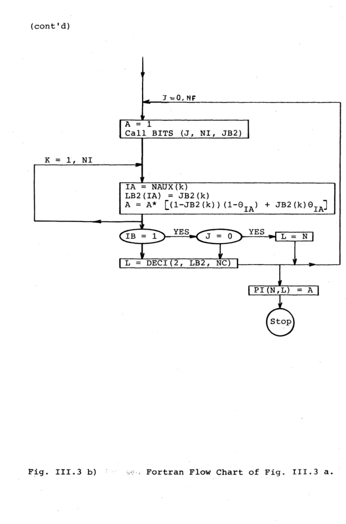
A schematic way showing how to compute the transition probabilities using these rules is shown in Fig. II-3. A flow-chart showing how to compute row n, of the probability transition matrix, when the decision is "go to state m", is shown in Fig. III.3 b). In the flow-chart we assume that we have available a subroutine called BITS such that given

n, a number, and NC number of components it returns the base 2 representation of n with NC components. The calling

L = DECI(k, LBk, NC)

such that given a vector LBk with NC components it returns the number L whose representation in base k is LBk.

These subroutines are given in Appendix C.

The simplifications explained so far can produce a great saving- in computation because, for instance, in the first case presented, only 2 of the 25-1 = 31 components-are different from zero.s

The optimization procedure for each starting state will consist then in the computation of the non null probabili-ties for the initial state row for every possible transition; taking scalar product of these non null probabilities by the corresponding costs - to - go and choosing the smallest result. The decision giving place to the smallest product is the optimal dec-ision for that initial state and the product added to the per unit t:ime cost for that state wi1 produce the next (backward) cost - to - go.

The flow chart of fig. III-4 shows the set of operations involved: in the: optimization process. In the next section we will show how this model can be easily extended' to problems with constra~ints- in the state space.

Initial State = n

Decision "Go to state m"

Write n and m in base 2 with NCdigits ni, mi are the iths digits respectively

Decision vector u(t) = n e m

Decision variables ui(t) ={i (t) if n. = 1 ci (t) if n=₁

Call I to the set of subindeces such that ui(t) - a(t) (i.e. ni = 0) and ai(t) = 1 NI = number of elements in I

Form the decision vectors u (t) where v = 1,..2 N I according to

n. = 1 or

u Mn i = n

_n

_{and ai = O}

i (t) =

vth combinationof? O's and l's in places where ni = 1 and ai = 0

1 = n 0 u (t) L ={1} , 2N I different l's The non null probabilities in row n when decision is "go to state m" are

m

nl (t) =N Oj (t) _k (1 - Ok(t)) VlEL

nij k

where j I and aj = 1 in uV(t) ke I and ak = 0 in u (t)

Fig. III-3 a) Flow-chart showing how to construct the

non-null probabilities of row n when decision is "go to state m"

State N

Decision "go to state m"

Call BITS (N,. NC, NB2) Call BITS (m, NC, mB2) NI = O N1 =O I DO I = 1, NC

N1

"-

_N1

+

₁

NB2 (I)=

1

NI Nb +- 1 'NAUX (NI) = I YES ,L YES NJBIB 2N _{I ,} _F 2.

(cont'd)

-=0, N0

A =1

Call BITS (J, NI, JB2)

K -1, NI

IA = NAU'X(k)

LB2(IA) = JB2(k)

A = A* (1-JB2(k)) (1-OIA) + JB2(k)(3IA]

YES YES LEN

Fig. 11. bFoL=wh N

L = DECI(2, LB2, NC)

-PI(N,L) = A

DATA: NC,T, C_i, Cij, 0_{i (}t) i, j = 1,..NC t = O.,1,..T M = 2NC-1

Compute Terminal Costs, V(T) using Fl.ow-Chart Fig.. III-2

I I

Steps backward in time Repeat from t = T-1 to 0

" "- Rows of transition matrix ' Row n corresponds to initial state n

Repeat from n = 1 to n = M

.ecisions: "go to state m'I Repeat from m = 1 to m = M:

Compute non null 'probabitlit-ies of row n:.

-Pl(t) when decision is "go to state mi", 'using flow-chart of Fig. III-3.

Compute the scalar product t) LP nl(t) V* (t+1)

Choose the smallest Rm (t) = R (t)

n n

"go to state v" is the optimal decision at time t from state n

Compute per unit time cost Xn(t) using flow-chart of Fig. III-2.

- V*(t) = f(t) +c 4 Rt(t)

Vector of costs to go at time tP

III-5. Constraints in the State Space

The problem formulation and the model described will allow us to handle easily constraints in the state space. These constraints may take the form of a maximum number of copies allowed in the sysitem at any instant of time -or,

not allowing copies of 'the file simultaneously in two. or

.more given. computers.

* Far instance., if g.iven ,a network with three computers (NC=3),;, three copies are not allowed in -the system simul-:taneously then state 7 will be taken out of :the set of

admissible states; if on the other hand, the restriction is that :there cannot be copies simultaneously in compupterQs 1 and 2, ;then state 6 is taken out of the state ..space.

One example of these types of constraints.was presented before when state 0 was not allowed. Therefore, unallowed states will be treated here in the slame way .state .0 ,was treated before. To gain some insight we present.an example:

Consider-a network with .four computers (NC=4). If the present state is .1 = (0 00 1) and the decission i·s

u(t) = (1 1 1 0), then the intended state is 15 = (1 1 1 1).

1 :l e2 a3 2 4 15

(-O 0 - 1) : ' (1 1 1 1)

1 1. 1 0

If there is a request from computers 1 and 3 but not from-computer 2., the system will, go to state (1 0 1 1) = 11 and this event will occur.with probability. 81(1- ₂):8₃.

Suppose now that state 11 is not allowed, then another decision has to be made. The situation is such that any

state of the form (a o b c) can be reached where a, b and c can be 0 or 1 (but not all three equal to 0). Nevertheless, considering so general a decision at this point will make the problem very complicated, therefore a decision to remain

in the same state will be considered. This is a particular case of the whole set of possible decisions. This kind of decision will give to state 11 the same treatment as to state O,as suggested, before.The probability of remaining in one state will now be composed of the following terms: Prob{remain in same state}= Prob{going to this state}+

+ Prob{going to state O} + Prob{going to not allowed states} (3.39) In the generat algorithm we will eliminate the rows

and columns corresponding to unallowed states and add their probabilities to the diagonal terms. It should be noticed that some extended simplification properties, similar to the one obtained in (3.16), could be obtained from the new

unallowed states.

For instance, for the example above where state 1 was the current state and state 11 was not allowed, we have that

a1(-a2)a3(1-c_{) 4} =

0

(3.40)

if, moreover, state (1 0 0 1) = 9 were not allowed as well, then

and from these two equalities

(1-Ca ₂) (1-£4) = 0 (3.42)

An illustrative example where these facts are applied is studied in Appendix B for the case of a network with two computers (NC=2). It is shown there that if we restrict the system to have only one copy at any instant of time the backward equations simplify to the equations given by A. Segall in El1], where the restriction was to operate with only one copy.

CHAPTER IV

UPDATING TRAFFIC AND NODE FAILURES

IV-1. Updating Traffic

The updating traffic consists of requests generated at some nodes after a request of the file, with the only

purpose of modifying, partially or completely, the content of the file, With this definition it is seen that the updat-ing information generated at any node, should be sent to

all other nodes that possess a copy of the file.

It will be assumed, for the present study, that, 1) This kind of traffic is generated at any node as

a fraction, of the query traffic of this particular-node. In general these fractions can be time

depen-dent variables. If we denote them by Pl(t), P₂(t), - - PNC(t)

the rate of updating traffic generated from node i at time t will be then

p i(t)Gi(t)

2) The updating traffic is implemented before the decision has been activated but after the request has taken place. The sequence of events is

Computation Requests Implementation Activation of

of optimal- come of generated optimal decisions

controls' updating

traffic

t- t' t

Fig. IV-1. Sequence of events including updating traffic

With-probability pi(t) an updating of the file is generated at any computer i that requested the

file and is sent to all computers that will keep a copy at time t+l..

3) We will assume that there is no conflict between the updating commands coming from different com-puters. This'is sometimes a serious problem in a practical case because it can force us to blockl requests, while some updating is being,done in order to avoid the processing of some old, and then use-lesas or-even conflictive, information.

Under assumptions 1) and 2) we can say that updating traffic is not a function of present state, but

only of present rates and subsequent states (as we will see in sections IV-2 and IV-3, this property is

not true if we include the possibility. of node failures). The only change to take place in the recursive equations will be in vector V*.(t+l) that will have some extra terms added-to its components.

N-1 V (t+l) + Pk(t) 8m (t) CkN k=l N V*(t+l) + Pk(t)k(t) CkN_ 1 k=l k#N-1 . N V (t+l) + Pk(t)Gk(t)

E

C

=V* (t+l)+R(t) k=l 1lI(j) (4.1) lfk . N N MV k ( t )k(t) k Ckl k=l 1=1 1lk

Here I(j) is the computers containing a copy at state j or in other words the set of subscripts corresponding to l's in vector state j. We are assuming here that the only charge involved in up-dating a copy at computer i by computer j is the transmission cost C...

The recursive equation will now be