Dynamic performance of magnetically levitated rotors

I

Dynamic Performance of Magnetically Levitated

Rotors

by

Benny Wahjudi Tjahjono

Submitted to the Department of Mechanical Engineering

in partial fulfillment of the requirements for the degree of

Master of Science in Mechanical Engineering

at the

MASSACHUSETTS INSTITUTE OF TECHNOLOGY

May 1995

©

Massachusetts Institute of Technology 1995. All rights reserved.

;?)

k

Author

...

Department of Mechanical Engineering

May 12, 1995 -f

Certified

by...

7Y

'?

Accepted

by...

Kamal Youcef-Toumi

Associate Professor

Thesis Supervisor

Ain Sonin

Chairman, Departmental Committee on Graduate Students

.. ASA6;US8r TTS INSTITUTE

OF TECHNOLOGY

Dynamic Performance of Magnetically Levitated Rotors

by

Benny Wahjudi Tjahjono

Submitted to the Department of Mechanical Engineering on May 12, 1995, in partial fulfillment of the

requirements for the degree of

Master of Science in Mechanical Engineering

Abstract

Magnetic bearings are selected as the physical systems because of the recent tremen-dous research activity in their use in high performance machines. The input-output characteristic makes such a system inherently nonlinear and unstable, so it is neces-sary to implement a desired control to it. However, if the system dynamic behavior and the limitations from the control system hardware as a whole are not incorpo-rated into the electro-mechanical and the control system design, the desired system performance may not be realizable.

This thesis treats the equations of motion of a rigid, horizontal rotor magnetic bearing system. Through LQ feedback linearization and describing function method-ology to approximate the saturation nonlinearity at the input level, the open-loop system characteristic is analized. This system is then simulated to demonstrate dis-turbance rejection properties and its robustness to parameter uncertainty and un-modelled dynamics. Such procedure results in the information of the performance limitation of a magnetic bearing system for the purpose of any further implementa-tion of its control design.

Thesis Supervisor: Kamal Youcef-Toumi Title: Associate Professor

Acknowledgments

I am very grateful to my thesis supervisor, Prof. Kamal Youcef- Toumi for his advice and assistance throughout my thesis work. His ideas, comments, and suggestions have helped me a great deal.

Students involved in collaboration during my thesis work need to be acknowledged (in alphabetical order): Mr. Ali Yurdun Orbak, a graduate student has been helpful in assisting me with using LaTex; Mr. Jake Wetzel, a graduate student is continuing experiments with control of magnetic bearings; Mr. T-J. Yeh, a graduate student whose paper got me started with the project and has been a helpful lab partner.

Contents

1 Introduction

1.1 Advantages and Disadvantages. ... 1.2 Types of magnetic bearings ...

2 Rotor Dynamics 2.1 Introduction. ... 2.2 Imbalance ... 2.3 Balancing ... 2.3.1 Static Balancing. 2.3.2 Dynamic Balancing ... 2.3.3 Flexible Shaft Balancing ... 2.4 Gravity Effect ...

2.5 Gyroscopic Effect ... 2.6 System Identification ...

2.7 Asymmetry Of Rotating Shaft Parts. 2.7.1 The Free Vibration ... 2.7.2 The Forced Vibration ... 2.8 Shaft and Mount ...

2.8.1 Flexibility ... 2.8.2 Damping ... 2.9 Instability ... 2.10 Critical Speed ...

2.10.1 Coupled Critical Speed ...

8 9 10 13 13

... .. .13

... . .23

... . .26

... ..33

... ..37

2.11 Whirling ... 3 Performance Analysis 3.1 Nonlinear System ... 3.1.1 Current Limitation 3.1.2 Magnetic Saturation 3.2 System Identification .... 3.3 Summary ...

4 Simulation and Results 4.1 Introduction ... 4.2 System Parameters ... 4.3 LQ Regulator ...

4.3.1 LQR Design with Rel 4.4 Saturation Limit.

4.4.1 Results...

4.5 Stability: Popov method . . 4.6 Stiffness ...

4.6.1 Results...

4.7.1 Results...

5 Conclusion and Recommendation

A The Describing Function of Saturation Nonlinearity

B Magnetic Force for Bearings

C Open-loop Matrices: Numerical Results

42 42 42 44 46 57 59 59 59 62 71 76 79 81 83 84 86 87

... . .90

...

...

...

...

...

...

...

...

...

...

...

...

...

...

...

List of Figures

2-1 Static balancing model ... 15

2-2 A rotor that is statically out of balance ... 16

2-3 Correction planes. ... 18

2-4 Balanced disk on a massless, horizontal elastic shaft ... 21

2-5 Gyroscopic Movement ... 22

2-6 The Fixed and Rotating Coordinate Systems ... 23

2-7 Possible configurations for steady motion of a disk ... 33

2-8 Damper and Spring ... 34

2-9 Rotating disk with a spring-restrained mass in a radial slot ... 35

2-10 Disk on flexible mounted bearings ... . 36

2-11 Lissajous figures traced by a point on a shaft at a given longitudinal station undergoing transverse vibratory motions at the same frequency on two planes ... 41

3-1 The Relationship between the Control u and the Coil Currents II and I 43 3-2 The control current setup in the radial direction ... 46

3-3 A Rotor Model ... 49

4-1 The open-loop roots ... 62

4-2 Linear Quadratic Regulator Design ... 63

4-3 LQ Loop ... 65

4-4 LQR Design: Closed-loop Poles ... .. 66

4-5 LQR Design: Frequency Domains, p = 10-_{3 ... 68}

4-6 LQR Design: Frequency Domains, p = 10 -3 ... 68

LQR Design: Initial Value, p = 10-3 _...

LQR Design: Disturbance Rejection Test, p = 10-3... LQR-design Roots ...

LQR Design: Frequency Domains, p = 10

-3, b = 100 ... LQR Design: Frequency Domains, p = 10- 3_{, b = 100 ...}

LQR Design: Initial Value, p = 10- 3, b = 100 ...

LQR Design: Disturbance Rejection Test, p = 10- 3_{, b = 100}

LQR Design with Saturation Limit ... Closed-loop System ...

A saturation nonlinearity ...

Closed-loop transfer function, r = 0.5, k = 1, tol = 0.006 . . Closed-loop transfer function, r = 0.5, k = 2, tol = 0.03 ... Closed-loop transfer function, r = 0.3, k = 1, tol = 0.01 . . . Closed-loop transfer function, r = 0.3, k = 2, tol = 0.03 . . . Stability Checking ...

Minimum stiffness, without any describing function element Minimum stiffness, r = 0.5, k = 1, tol = 0.006 ...

Minimum stiffness, r = 0.5, k = 2, tol = 0.03 ... Minimum stiffness, r = 0.3, k = 1, tol = 0.01 ... Minimum stiffness, r = 0.3, k = 2, tol = 0.03 ... Disturbance-to-output, r = 0.5, k = 1, tol = 0.006 ...

Disturbance-to-output, r = 0.5, k = 2, tol = 0.03 ... Disturbance-to-output, r = 0.3, k = 1 ...

Disturbance-to-output, r = 0.3, k = 2 ...

A nonlinear element and its describing function representation A saturation nonlinearity ...

Saturation; axisl = , axis2 = Magnitude ...

Coil Windings for an Electromagnet of a Bearing ... Coil and Contour for Faraday's Law ...

4-7 4-8 4-9 4-10 4-11 4-12 4-13 4-14 4-15 4-16 4-17 4-18 4-19 4-20 4-21 4-22 4-23 4-24 4-25 4-26 4-27 4-28 4-29 4-30 A-1 A-2 A-3 B-1 B-2 69

...

69

....

100

....

100

Chapter 1

Introduction

The magnetic bearing setup consisting of four magnets is widely manufactured in order to apply the non-contacting type control force to a rotor system during oper-ation. A magnetic bearing typically consists of an even number of electromagnetics with alternating north and south poles wrapped around the axis of a rotating shaft. The poles are oriented facing the axis in a journal bearing and parallel to the axis in a thrust bearing [9]. A setup generally consists of two separate systems, which are an axial positioning system (thrust bearing), and a pair of radial positioning systems (journal bearing). If it is necessary to protect, in event of power failure or loss of criti-cal system, then an auxiliary bearing (catcher bearing, or backup operational bearing) could be augmented to the system.

Journal and stator, like those of an induction motor, are stacks of ferromagnetic lamination so thin that its eddy current effect becomes negligible. A journal is a plain disk, while a stator is wound with magnetizing coils to form pairs of north-south poles; each is driven by a separate power amplifier, which actively controls the current in the coils. A rotor is suspended and stabilized within a stator. Steady state (bias) current is induced to the magnetizing coils. The control current is superimposed on the bias current to regulate the attractive force on the journal. The bias current is much larger than the control current, and the total current never changes its polarity

in a power amplifier1. If the journal excursion is relatively large in gap, then the linearized controls are essentially uncoupled in two independent directions [3].

1.1 Advantages and Disadvantages

Magnetic bearing systems are indispensable for

1. suspending and spinning the shaft at high speed operation,

2. the ability to utilize thinner and less rigid shafts which results in reduced weight

and increased in design flexibility,

3. its frictionless nature resulting in high temperature or vacuum condition oper-ation,

4. lubrication-free operations resulting in the savings in construction time,

start-up time (e.g. oil flushing), maintenance time and related maintenance free operations,

5. having the adjustable damping and stiffness which mainly depend upon the frequency,

6. permitting the active control of bearing dynamics characteristics which lead to

the foundation of an external control algorithm,

7. having the existing wide range of possible dynamic characteristics enabling the placement of the critical operation speeds of a particular machine,

8. optimization at several different speeds by merely changing the constant system parameters.

On the other hand, the disadvantages include 1. high initial equipment cost,

2. lack of the operating data to confirm the performance expectations, 3. unstable characteristic.

Due to their unstable nature, they require external electrical control to regulate electromagnetic forces acting on bearings2_.

Nowadays, the magnetic bearing applications are found in some industrial, mili-tary, and space systems. The advancement in rotor and material technology has re-sulted in some applications such as turbines and compressors, rotating at the speeds previously unattainable, e.g. maglev (magnetically levitated) high-speed train.

1.2 Types of magnetic bearings

Three main types of magnetic bearings [9]:

1. active magnetic journal bearings, such in turbo-machinery. Its advantages over fluid film bearings include the low power loss, the elimination of lubrication systems, and the control ability of the bearing forces to minimize vibration. 2. passive magnetic bearings.

3. hybrid magnetic bearings, i.e. eddy current magnetic bearings.

An active magnetic bearing generally consists of a stationary electromagnet called stator, and a rotating ferrous material called rotor that are used to allow a shaft to be suspended in a magnetic field. The shaft position is maintained dynamically. Such process is done utilizing sensors that provide continuous feedback through control and amplification system to the electromagnetic poles to suspend the shaft. One example of its applications is a gas compressor.

Based on the types of configuration (either of the two force mechanism), in con-ventional bearing, the attractive force is generated between a magnet and a piece of magnetic material as in fluid film, ball or rolling element devices, where load capacity is determined by wear and heating. Such scheme is highly unstable; it requires feed-back control to obtain a desired stiffness characteristic[4]. Another scheme is based on the force of repulsion, which is caused by eddy current induced in a conducting but non-magnetic rotor and some stationary magnets driven by a time-varying current. Lately, magnetic bearings were invented where their specific load capacity is only due to the saturation of the magnetic material.

The primary role of any bearing is to restrain the motion of the supporting ro-tor in response to any applied loads, and also the load response to satisfy a given set of performance constraints3 However, no explicit load capacity requirement has been established for stability (by the dynamic properties of the bearing itself) on the bearings.

The rotating parts, while having the same characteristics as the stator and rotor of an electric motor, are able to provide a long life without requirement for planned maintenance. The bearing is not sensitive to many process fluids, or within certain limits, to the process fluid temperature or pressure. In a submerged motor concept, the complexity associated with gas/lubricant seals or gas buffering is eliminated. The on-line control of the rotor allows loading, eccentricity, shaft position and vibration to be controlled and remotely monitored for both short and long terms. The machine vibration reduction will extend the operating life significantly and reduce cost of rou-tine maintenance and repair. The system reliability will also be improved, and could be enhanced further with redundant controls and power supplies. Furthermore, the shaft speed rangle will be unlimited by circumferential speed and bearing limitations

[12].

This thesis will investigate the feasibility of electromagnet suspension of a rotating shaft without mechanical contact. In such configuration, there are many possibilities to implement a wide variety of modern control strategies under computer control

3

[7, 11].

Chapter two describes the dynamics analysis of a rotor system. The rotor is as-sumed to consist of a rigid disk on a flexible shaft (Jeffcott model). Taking into account the mass unbalance and shaft flexibility, the general fomulation is then de-rived for this specific model of rotor. Some important dynamic features of a rotor due to its critical speed, whirling, and asymmetric shaft are also discussed.

Chapter three describes the performance of a magnetic bearing system. The rigid disk model derived on Chapter 2 is extended for the rigid body of a rotor to include the gyroscopic effect motion. The inherently nonlinear system is formulated and

linearized at its equilibrium operating point. The system matrices is then set up to analize the nominal performance.

Chapter four presents the numerical and simulation results. The LQ regulator methodology is utilized to stabilize the open-loop system. The describing function element to represent the current limitation at the input is then applied, and the system is analized to determine its overall closed-loop performance.

Chapter 2

Rotor Dynamics

2.1 Introduction

This chapter covers some fundamental aspects of a rotor from its static and dynamic perspectives. Sect.2.1. illustrates the cause of static, dynamic, and flexibility im-balances, while sect.2.2. demonstrates how to overcome such imbalance types by the so-called balancing methods. Rotor imbalance can result in a gravity effect (sect.2.3.) that will generate a pulsating torque on the shaft. Gyroscopic effect upon the rotor critical speed is also determined in sect.2.4. Furthermore, the influence of asymmetry of rotating shaft parts on the critical speeds is remarked in sect.2.5. In sect.2.6., the flexibility of the shaft and the mount could be represented as elastic springs, while in sect.2.7., the shaft and mount damping are represented as radial dampers. The dynamic instability is partly determined by the shaft deflection (sect.2.8.) which de-pends upon frequencies. More importantly, the critical speed and the rotor natural lateral frequencies are covered in sect.2.9. Shaft whirling is mentioned in the last part

(sect.2.10.).

2.2 Imbalance

In any real system, when a disk is set on an infinitely rigid shaft, there is always an offset distance of the center of mass from the geometric center of its concentrically

round section due to mass imbalance. Such offset distance is called eccentricity (e)

[14].

There are three (3) types of imbalance:

1. Static imbalance, where the center of gravity is offset from the axis of rotation while the principal axis of inertia is still oriented in the same direction as the axis of rotation.

2. Dynamic imbalance, to describe the angular misalignment of the shaft principal axis of inertia with respect to the axis of rotation. Both static and dynamic imbalance are generally present due to manufacturing tolerances.

3. Flexibility imbalance due to the shaft flexibility when it is rotating near the vicinity of its critical speeds.

Imbalance will affect the internal friction of most conventional rotors such as the slippage between one set of contact surfaces of such as built-up rotors may not begin at the same operating speed as between another set. Moreover, an increasing imbalance may enact more sources of internal friction for a given operating speed [14].

In a high speed machine, any small geometric imbalance will cause a large oscil-latory force to transmit to the supporting structure, while any large imbalance will increase the possibility of fatigue failures in the rotating shaft or premature bearing wear and seizure.

2.3 Balancing

2.3.1 Static Balancing

Static imbalance can be detected without acting the rotor into rotation. If a statically imbalanced shaft with concentrically round surface is set across two perfect level, flat and parallel supports, then the rotor will rotate until its center of the mass is at the lowest point. The method of balancing is then to affix a mass 180 degrees away from

x

3

rT/

Y

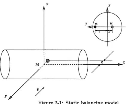
Figure 2-1: Static balancing model

this center of mass. In practice, the rotor is propped on a balance machine and the weights are moved around to the points where the rotor balances on a level.

The imbalanced shaft (Fig. 2-1) has the following values for the center of gravity:

xg = 0, yg = -, zg = 0 (2.1)

The center of gravity, with an additional mass affixed on the surface of the shaft 180 degrees away, is given by

M - mr

x =g= 0, Yg = +M (2.2)

where M is the original rotor mass, and m is the affixed mass. It is the interest here that m is set at a distance equal to Me/r, so that the rotor will be statically balanced y = 0.

2.3.2 Dynamic Balancing

In order to carry out the method of dynamic balancing [14], the rotor is mounted on the mobile platform of a balancing machine. By a dynamometer or such, the rotor

i

---I = =..

d a Z

midstation

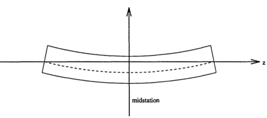
Figure 2-2: A rotor that is statically out of balance

is let spin up to speed and vibrate 1. The balance points are noted by computer and

the proper balance weight spots are then indicated by measuring the amplitude and phase of platform vibration.

The components of the balancing machine include

1. mechanical platform assembly to reflect the necessary degrees of freedom of a rotor,

2. a driving system to set a specific speed of rotation,

3. measuring devices to carefully detect the motion of the platform, and

4. an accurate device for adding and removing material at specific locations on the rotor.

Theoretically, for a rigid rotor, the cross product of inertia must equal to zero, that is

I. = IY = 0 (2.3)

'It is an obvious sign of imbalance.

The mass products of inertia, I,, and Iy, are given by

Ixz IsZ = fv xzdm JVldm (2.4)(2.4)

·

If this is true and the x and y coordinates of the center of mass are also zero, that is

xg = g = 0 (2.6)

then the rotor is both statically and dynamically balanced.

If the shaft center line is slightly bowed into an arc symmetrically about the normal to the rotor midstation 2-2, then the rotor will be statically out of balance but not dynamically 2. Any inhomogeneity would cause dynamic imbalance unless the dynamic distribution is again symmetrical with respect to the midplane.

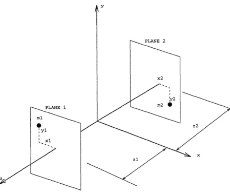
If a rigid rotor is dynamically out of balance, two correcting weights are affixed in two arbitrarily positioned planes, which are called correction planes (Fig. 2-3), normal to the axis of rotation and located at z = zl and z = z₂. The correction masses are denoted as m and m2, and located at (x, yi, zl) and (x2, Y2, z2) respectively. If the

original imbalanced rotor has mass M and cross products of inertia I and Izy, then the balanced cross products of inertia (with the correction mass added), are

-newr

-=

Ixz

+ mlxlzl + m2x

z

,

(2.7)

IyneW = Iyz + mlYlZl + m2Y2Z2 (2.8)

y

PLANE 2

Figure 2-3: Correction planes

The coordinates of the new center of mass are given by

new = Mxs + mmlx + 1 + m2x2

(2.9) x9 M

+m

new Myg - mlyl 22 (2.10)

m+M ±m ₂

To have the rotor both statically and dynamically balanced, it is necessary that

xnew = 0 = mlX + m2X2 - -M-c (2.11)

ynew = 0 m l miy + 2Y2 = -Myc (2.12) InewZ = 0 = zI(m₁x₁) + z₂(m₂x₂) = -Ix (2.13)

ynewz = 0 => Zl(mlYl) + z2(m2Y2) = -Iyz (2.14)

As implicitly shown above, the coordinates x1, x2, Yi, Y2, z1, z2are determined by

removal. The formula proves that it is possible to balance the rotor by using two masses, given the xc, y, I, and Iy 3.

2.3.3 Flexible Shaft Balancing

When the rotor is rotating at a speed in excess of the lowest natural frequency, it can no longer be considered rigid, because the true position of the mass center and its instantaneous cross products of inertia will be different for each operating speed. In order to account for this effect, the balancing is determined according to the particular vibration modes, assuming that the rotary inertia effects of the rotor cross sections and the attached disks may be neglected. The drawback of this method is that the natural vibration frequencies and mode shapes of the rotating shaft are the same as those of the standstill shaft. The fundamental aspect of this so-called modal balancing is to use the natural vibration modes as generalized coordinates. The modal equations have the inherent orthogonality, making it possible to uncouple equations and determine the necessary correction weights to balance out the reactions of the lower modes.

Modal Balancing

A theoretical modal balancing technique may not always overcome vibration entirely at the required range of operating speeds, even if the gyroscopic moments are com-pletely negligible. The generalized imbalanced force at its source, weighted by each particular modal deflection shape, acts as the only driving function in this normal mode analysis. If the imbalance distribution has sharp variations or if its shape is like the deflection shape of one of the higher modes, the generalized force that excites the higher modes may be large enough. Unless those modes are included in the balanc-ing procedure, the dynamic bearbalanc-ing reactions may still be large. A modal balancbalanc-ing technique using only the lower modes is sufficient only if the harmonic content of the imbalance distribution is not too large [14].

3In practice, it is difficult to determine these predetermined constants experimentally without already having balanced the rotor.

Harmonics Balancing

The method of harmonics balancing, as combined methods of balancing states is stated as follows: a massless flexible rotor holding r concentrated masses, supported on b bearings, with an imbalance, can be entirely balanced by weights distributed in n = r + b different planes along the rotor length. This method of complete balancing eliminates any dynamic reaction in any bearing at any rotating speed, given that the imbalanced masses are small compared to the whole mass of the rotor, and that

the flexure due to the imbalance is small compared to the eccentricities of the static imbalance. For futher information in this harmonic balancing method, one may refer to [14].

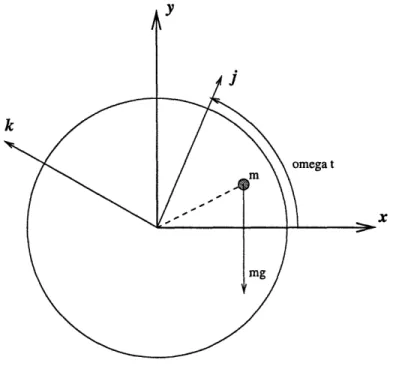
2.4 Gravity Effect

If the axis of rotation were horizontal, and the disk had imbalance, the force of the center of gravity would become a transverse excitation source. Viewed in the

stationary frame, the force is directing downward, but in the rotating system, it is sinusoidally varying with frequency of vibration, that is

-mg sinwt,

in the j direction

(2.15)

-mg coswt,

in the k direction

(2.16)

A different way of looking into this gravity effect on a rotating horizontal shaft is to consider the frequency of the exciting force is zero in a fixed coordinate system, but once-per-revolution in the rotating system. In other words, the imbalance would initiate a once-per-revolution pulsating torque on a horizontal shaft.

2.5

Gyroscopic Effect

If the disk doesn't remain in one plane when it is rotating (particularly at higher speeds), then the so-called gyroscopic effect must be taken into account of the rotor

v

i

omega t

X

Figure 2-4: Balanced disk on a massless, horizontal elastic shaft

dynamics. Loewy et al. states in [14] that gyroscopic effect may increase or decrease

the critical speeds of a rotor significantly, depending upon the operating speed, size

and geometry of the gyroscopic disks, and disk location on the rotating shaft. The gyroscopic moment is determined as proportional to the time rate of change of the

shaft's transverse angular displacement and directed 90 degrees from that of

trans-verse angular velocity. Therefore, it is necessary to consider the simultaneous bending

of the shaft in two planes, while the polar mass moment of inertia about the shaft center line is an important parameter also.

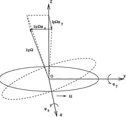
According to Dimentberg [5], the movement can be in the direction of the rotation of the shaft, which is called forward precession, or in the opposite direction, which

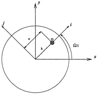
is called reverse precession. If the disk rotates with Q and deviates about the z axis by an angle p, then the movement tends to displace the positive end of the z axis towards the 0t axis.

\- - - - - -I1 1% II3Q D -z Iplpo y I (Py /' X

Figure 2-5: Gyroscopic Movement

disc mass as Ie and Ip, the displacements of the disc center along the fixed axes and the angles of rotation as x, y, cp, and Ty, while the angular speed of the disc as , the projection of the force F and the moment L of the movement on the axes are then given by Fig. 2-5,

Fx Fy Lx LY IPn Ln =

ma

=

Iex

+ IpQ(py

=0

Equating the time derivatives to the projections and the moments of the external I I I I I I I I I I

X

0

Figure 2-6: The Fixed and Rotating Coordinate Systems

forces respectively, acting on the disc or, which is the same, to the values with the opposite sign of the projections and the moments of the inertial forces, transmitted

from the disc to the shaft, the equations for the disc movement are

mx

= -Pr,

(2.23)

my

= -P,

(2.24)

Ie4,- IpQOl = -My, (2.25)

Ie¢X

+ IpQy

= -M.

(2.26)

with -IpQo, and IpQy as the gyroscopic terms.

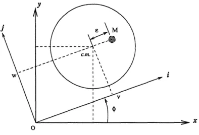
2.6 System Identification

Following the assumptions made in [14], the static location of the standstill rotor is

at 0, i.e. x = y = 0 or v = w = 0. During the rotor movement, the shaft axis is considered deflected from this standstill location. The rotor is running at a constant

angular velocity, i.e. 0 = Qt.

r

= ( + )i + j

(2.27)

= (x + e cosQt)x + (z + e sinQt)y (2.28)

i

=v

ii + bj + Qk x [(e + v)i + wj]

= ( - Qw)i + ( + v) Qbij

(2.29)

Differentiating again, the above equation results in the acceleration of the rotor mass, M. After simplification, the equation is

r

_2Qtb

_2Qvi)j

_(2.30)

= (i - eQ2cosQt)x + ( -_ eQ2

sinQt)y

The elastic restoring force acting on the system is provided by the shaft stiffness

f,

= -(vi + wj)

(2.32)

= -(xx

+ yey)

(2.33)

where c is the approximated linear spring constant.

The internal friction force, which is viewed as the friction associated with the

rotating coordinate system, is given by

fi =-c,(9i + bj) (2.34)

-

-c[(± + Qy)x + (

-

Q

Qx)y]

(2.35)

and the external friction force, which is viewed as the friction associated with the fixed coordinate system, is given by

=-ce(±x + y) (2.37)

where ci and c, are the approximated internal and external friction constants, respec-tively. In the case of rotors of magnetic bearing systems, ci and ce are zero, due to the frictionless nature of the systems.

The relationship between (x, y) and (i, j) coordinate systems is established via rotational transformation [8] as follows;

x cosq -sin v

[Y

sin

cos

w

Since the equation of motion in each frame of reference is

mi = f + fi + fe, (2.38)

then

Fixed coordinate system

i + Ce

ru

+ Ci

+

-

= Q2e

sinQt,

(2.40)

m

m

m

dt

sinQt

Rotating coordinate system

+

____

m

m

m

-(i - Q

2

₎

Using complex representations =

Fixed coordinate system

y + jz and u = v + jw, the equations become

ci + ce. iQ =

ijS ii -

3-

m m m Rotating coordinate system

u+

cU

+ ( -

2)U

+

322

=

e

(

m m m

Then, a particular solution is obtained by setting 7 = oe3a_{t and u = uoe3at:}

Q2 ;

710

= (

and

-Q2z

= A(42e_

O)2

+ (

2f

2.7 Asymmetry Of Rotating Shaft Parts

2.43)

2.44)

2.45)

2.46)

Here is the work of Ariaratnam [1]. He analyzed the vibration of unsymmetrical rotating shafts whose flexural rigidities are unequal in the principal directions. The bearings are considered symmetrical in this case.

or = 2, = 0, (2.41) (2.42)

d

From Fig.2-6, it is understandable when the shaft is assumed to be unsymmetrical, the equations in (y,z) will contain periodic coefficients, while those in (u,v) will not. Obviously, the latter is easier to handle. The equations are then

ii

-

Q2(u

+

al)

- 2v

=

(a

u -

) - a(i - gv) - i - g sinQt (2.47)

EI

Vi _ 122(v + a2) + 2F =--a (v - vo) - a(b +

Qu)

Pi

-

g

where m is the constant mass per unit length of the shaft, and El1,2 are the

flex-ural rigidities of the shaft cross section for bending in the planes of OXV, OXW, respectively.

In deriving the above equations, it is assumed that

1. the deflection amount of u, v, u0, and v0 are assumed to be small so that the

Euler-Bernoulli theory of bending may be applicable,

2. the damping forces acting on unit length of the shaft are assumed to be viscous and containing the external damping of magnitude (-ma) times the transverse velocity of E relative to the fixed axis, and the internal damping of magnitude (-m/) times the transverse velocity of the cross section relative to the rotating axis.

By assuming Q = a = 1 = uo = vo = 0, the free, undamped, transverse linear vibrations in the principal directions of a perfect standstill shaft of unsymmetrical cross section are given by the equations as follows:

EI1 a4u

u/i+

- =0

(2.49)

v + 4 _{0 (2.50)}

m 194 From Eq.2.49, the solutions are of the form

The spatial function (x) satisfies the equation d4_{0 k40 (2.52)} dx4 where mw2

=k

EIx

From Eq.2.52, the general solution is

O(x) = A cos kx + B sin kx + C cosh kx + D sinh kx

(2.54)

where A, B, C, D are constants obtained from the limit conditions at the bearing locations.

Assuming that the mass unbalance is located at (a,, a₂) in the direction of (i,j), the functions can be expanded as series in the characteristic functions as follows;

00 al(x) = E a,,iq (x) (2.55) r=l a2(x) = Zar2 Or(X) (2.56) r=l oo

U

=

erlr(X)

(2.57)

where the Fourier coefficients anr, ar2, erl, and e2 are

ar =

a(x)qr(x)dx

(2.59)

ar2= JOa 2(x)Or(x)dx (2.60)

erl = j el(x)qr(x))d x (2.61)

The equations of motion are then obtained as follows:

i

+

( +

)ir +

(W2

_

2

)r -

2Q

-

Qqr

= Q2_{arl + Wrerl - gIrsinQt}

7r + ( +

)7r

aQtr

= Q

_ar2

₊

_W2er2

_{- g1rcost}

or in the matrix equation,

r &7hr (r 0 0

-(:x- )

0 O 0

arl

-gIr

sinQt

c,=&oefficients of the external and internal damping, w,=the natural frequency of transverse vibration

JD

fo

respectively

For asymmetrical shaft, wrl wr2, and the equations have to be treated as simul-taneous differential equations and solved by elimination of variables.

2.7.1 The Free Vibration

For the free vibration of the rotating shaft, the equations of motion are given by the complementary functions of Eq.2.63- 2.64; the general solutions are

;r

+

2Qr

jr

7

+

(ew

2

-

A type of possible solutions are of the form

&'(t) = PeAt, r (t) = QeAt

where A, P, and Q are constants, providing the characteristic equation

[A2±(a+

+

+

)A

+(w

+

[A2±qY-)+(w

r2

-

A

_{+ )AX}

A2

± ,+)(w2

A

According to Routh 's stability criterion, the solutions will be bounded at all times

if all roots of A have nonpositive real parts:

(c

(~~~

+ )(W2,

)r2

+

+ W

-

2Q

2

)

+

4aQ2

> 0

(wr1 - 22)(r22 - Q2) + a2Q2 > 0 (2.69)

Due to the frictionless nature and vacuum operating condition of magnetic bearing

systems, both external and internal damping are absent, i.e. c = characteristic equation (Eq. 2.67) is then reduced to

A4_{+ (W7}

1+ w2

+

= 0, = 0. The

and the corresponding roots are

1,2 = I + Lw 2) 2 i Q2(W21 + Wc22) + ( w - 2 (2.71)

If Q = 0, then A 2 are real and unequal. If w2# 1 Q :A w2₂, then Eq.2.67 gives four

fundamental solutions. When Q is outside the finite intervals Wrl < Q < wr2, (r = 1, 2, ...), A22 are both negative (all values of A are purely imaginary), and the solutions

will be bounded.

If = Wrl, w,2, (r = 1, 2,...), A = 0 is a double root of Eq.2.70, and the solutions are of the form

&(t)

P

t,

71r(t)

Q1

Q

t

(2.72)

which are clearly unbounded due to the factor of t.

The particular solution is then obtained from [1] as follows:

E2 + W2 2 Q42 ~2arl -ierl a

,.

+

sinft,

(2.73)

sint

(2.73)

r(t)

=

-a

122-2

(w

g'

(2.74)

2.7.2 The Forced Vibration

Recalling Eq.2.63 and Eq.2.64, i.e. the particular equations representing the forced

vibration due to unbalance, initial lack of straightness, and gravity. This forced motion will be unbounded for some causes as follows:

1. shaft imperfections, i.e. unbalance, initial lack of straightness.

Q = wrl, 1 = W2,

r

1,

2. effect of gravity

WrlWr2

=

2+2)X

r-=1,

2,

...

is considered the secondary critical speed.

2.8 Shaft and Mount

2.8.1 Flexibility

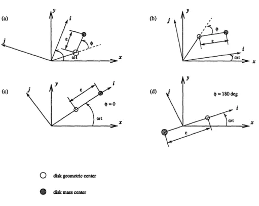
Consider a shaft configuration which consists of a disk, a massless elastic shaft con-strained to stationary (,y) or rotating plane motion (i,j). The bearings are placed at the origin, and the shaft is infinitely stiff in torsion. The shaft transverse (bending)

flexibility allows translational motion of the disk in the plane of rotation, which may lag (Fig. 2-7a), lead (Fig. 2-7b) by angle ;b, or be coincident with the shaft rotation

(Fig. 2-7c,d). Here, the effect of shaft bending flexibility could be represented as a linear spring. If the shaft bending rigidities are not polar symmetric, then there would

be different elastic restoring forces, although the magnitude of the displacements in

the direction of the linear springs were all equal. A shaft with significant difference in stiffness in any two directions would be subject to instabilities.

The flexibility effects due to shaft elastic properties and in the shaft bearings are quite similar. If the shaft has polar- symmetric stiffness and the bearing spring rates

are isotropic, these two dimensional descriptions become interchangeble. The shaft

stiffness would provide a steady radial force, and the bearing springs k = k would provide the same steady resultant radial force.

2.8.2

Damping

The structural damping of the shaft is represented as a radial damper (Fig.2-8) which is parallel with the springs, acting as a powerful dissipative medium. These damping forces, whether isotropic or not, act very differently from friction in the rotating shaft.

y i 10 (b) j x y £ ig

Y

A

to

0

disk mass center

Figure 2-7: Possible configurations for steady motion of a disk

As in the case of the shaft and mount flexibility, any constant amplitude circular whirl would not cause oscillation in the shaft spring, but continuously cycle the springs.

2.9 Instability

A system is considered unstable, when it is not subjected to external forces and has only free motion due to its initial conditions, but its motion develops indefinitely with time. Consider a disk that is perfectly balanced but contains a frictionless, radial slot, in which there is a mass m, restrained by the spring k, as shown in Fig. 2-9. The radial equilibrium of forces on the mass could result from a balance of centrifugal and elastic forces. mQ2(e + v) = kv (2.75) (a)

j

j

I

Figure 2-8: Damper and Spring

or

mQ2e e

v =

_k

=

- m 2 _in2 1

The elastic deflection v will be unbounded for any initial deflection e if the rota-tional speed Qd = y- , which can be considered as critical. If the mass is rotating

about a mean position e = 0 without vibration, then the Newton's second law yields

mi)

-kv

+ (k _ 2_{)v = O}

m

Viewed in the rotating system, the rotating natural frequency is

,_ - 2 = wn 1

WnR

=

It is obvious that the divergence speed Q2d occurs when the rotating natural

fre-(2.76)

x

Figure 2-9: Rotating disk with a spring-restrained mass in a radial slot quency is zero, when viewed in the rotating system. The solution of v is

v = volei w Rt + v0 2-e ic ' r t (2.80)

which shows that if Q > d = ~, one of the two terms will diverge. Thus, fd

represents the limit of a semi-infinite region from FQ = Od to Q = co.

2.10 Critical Speed

Rotor has certain speed ranges in which vibrations of large amplitude could occur, causing to operate harshly, transmitting large forces to the bearings and exhibiting considerable deflections of the rotor. The critical speed vibration requires external excitation such as provided by rotor unbalance. If the operating speed coincides with the rotor critical speed, then the large forces on the bearings may possibly cause bearing failure, or the resulting excessive rotor deflection may wipe out the internal labyrinth seals causing rotor failure and affecting unit efficiency. Dunkerley theorizes that if the rotor had any unbalance (which is generally unavoidable), then it would excite the natural lateral frequencies, generating high vibrational amplitudes if the

j

.-1 -\IX~10x

Figure 2-10: Disk on flexible mounted bearings

operating range should coincide to any of these values [13].

Fig. 2-10 above approximates a magnetically levitated horizontal shaft with mass

unbalance, where linear springs k and ky represent the magnetic bearing supports

in the direction of x and y axes, respectively. Assumably, each pair of supports for each axis could be represented by only one linear spring. The x, y axes are fixed at the undeflected bearing location. Letting k = ky = k, and Q = Qc =

k/rn

will grow unbounded in the absence of damping, and the solutions will be [14]

x 2e (A + t) sin Qct + B cos Qlt, (2.81)

2

Y

-Q e

(A' + t) cos Qt + B' sin Qt,

(2.82)

2

where A, A', B, and B' depend upon the displacements and velocities of x and y at time t = 0. The sum resulted of the two motions is a diverging spiral, so a, is also considered as a critical speed, and numerically equal to an undamped natural frequency. However, if Q > Qc, then the motion will be bounded, and the

corresponding ranges will be where the instabilities predictably will occur. Thus, only at the speed Q2 will result in a whirling divergence linearly with time, as viewed

in the rotating system. In case of the slotted mass, whirling divergence will result exponentially with time beyond the speed of 2_{d, and its rapidness will be determined}

by how far the unstable range of Q > Qd is entered.

2.10.1

Coupled Critical Speed

To investigate the rotor response during transition, the rotor angular displacement of

the rotating coordinate system is considered to include a specified angular acceleration

as [14] ¢ = aot + at2 . (2.83) Hence,

d[l] = Q

= flo + 2at,

(2.84)

The angular momentum of the disk about its center of mass is equal to its polar

moment of inertia times the angular velocity of the disk. The total moment of force acting about the center of mass is

Tk - ei x fe = (T + enw)k. (2.86)

The total moment must equal to the rate of change of the angular momentum, which is d [L= + IpQ];

T

= -New + Ip

(2.87)

= ,e(x sin - y cos) + IQ

(2.88)

Now, the coupled equations of motion lateral bending-torsion for an unbalanced disk at the center of a flexible shaft is considered, where the shaft is not rotating at a

constant speed. If the instantaneous angular rotation rate Q2 is provided by a steady state 1o added by a small perturbation , then the linearized equations of motion

in the coordinate system affixed to the shaft will be as follow (after dropping the multiplication terms of the first derivatives)

from Eq. 2.41 and Eq. 2.42

Ci

+

ie

+

(

-

2 -

2¢Qo)v

-

e (Qo

+

)w

-

2Qmo

m m m

= (0L + 2Qo0)e, (2.89)

' + Ew

+ (- - 2 - 22o)w

+ (Qo

+ )v

+ 2Qo

= °,

(2.90)

m m m

and from Eq. 2.87

Ip

-

rc.w + r,0 = T =0,

(2.91)

where the applied torque is assumed to be zero in generating these equations.

Assuming that a particular solution for the unbalance force consists of constants for v, w, and 0. Substituting into the equations after dropping the first and second derivatives, yields -Q0)vo - Me{wo = n2 (2.92)

m

m

+ (o)2

(2.95)

WV

(.

=

=

--Wo.

(2.97)

if 0 = , which is the undamped natural frequency of a critical speed. It shows that the classical critical speed is unaffected by the addition of torsional stiffness. Morever, the presence of external damping Ce will avoid the occurence of such critical

speed.

The secondary critical speed due to gravity is unimportant, because there is no resonance phenomenon at an operating speed near half the critical. If these conditions

are affected by the coupling of bending and torsion, then the equations of motion of the centrally located disk on a horizontal shaft are

mx = -x,

(2.98)

my = -y-

mg,

(2.99)

and

Ip + SAX + nCe(x sin - y cosb) = 0 (2.100)

Adding the terms of -mgsin(+Qot) and -mgcos(+Qot) on the right-hand sides of the rotating frame equations respectively, and introducing the complex notations u = v + 3w, and il= v - 3w, the equations of motion become

Ci + Ce (I 2 2e;(Q ~)

+

_m

m i +

(m- - 2o) + 32Qou

_m

+

3 (Ro

_m

+

)u

= (Q2 + 2Qo)E - 39e-3(O+ ot), (2.101)

Ip + 3 (u - ii) + Koq = 0. (2.102)

2.11 Whirling

Whirling is defined as the angular velocity of the rotor mass center. It is considered as a self-excited phenomenon. The exciting force for the case of shaft whirling, is provided by the frictional force, referred to as rotating or rotary damping, generated

between two contacting surfaces when undergoing relative sliding. When the

preces-sion rate is smaller than the rotational speed, the rotary damping force becomes a source of excitation, causing the whirl amplitudes to increase. If the rotor centerline

is moving with the same angular velocity as the mass center, then it is considered as synchronous precession; otherwise, it is nonsynchronous precession. It is generally

noted that whirling always occurs above the first critical speed [14].

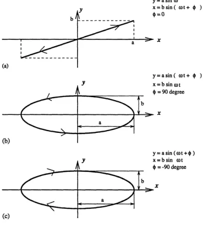
Observing transverse shaft vibration in two mutually perpendicular planes (Fig. 2-11), the frequency and phasing at a given point along the shaft length determine a closed curve, called Lissajous figure. It occurs both in the fixed and rotating frame.

If it happens in a rotating system and with non-zero phase, then the shaft center will appear to rotate. Viewed from the rotating system, if the rotation is in the same direction as that of the true rotational velocity of shaft, then it will be called a forward, advancing, or progressive mode. Otherwise, it will be called a reverse, backward, or retrogressive mode.

Describing the classical shaft critical speed phenomenon, forward whirl is a lim-iting case of zero apparent rotation of the shaft center in the rotating system. Loewy

et al. in [14] states that in a more complex phenomena, the forward or backward pre-cession, viewed from the rotating system, may occur at integer multiples of rotational speeds.

(a) (b) (c) y a Y Y y= a sin o x=bsin( t+ ) = x 2a.'x y=asin( wot+ ) x = b sin )ot 4 = 90 degree - x y= a sin( ot + ) x=b sin t I4 = -90 degree x

Figure 2-11: Lissajous figures traced by a point on a shaft at a given longitudinal station undergoing transverse vibratory motions at the same frequency on two planes

I - | !_ l l =l a ---i - S * , ,, ! - o Sc --- bl

---111-

Chapter 3

Performance Analysis

3.1 Nonlinear System

3.1.1 Current Limitation

To eliminate the complexity by multi control inputs of Ileft and Iright, and to ensure that power is not wasted due to unnecessary work done by the bearing, the following relationship described in [10] between the control uy and the coil currents Ileft and

'right is used,

Case 1. When control uy is between -uo and uo, i.e. -uo < uy < uo

(3.1)

Ileft = Io - 0.5_{uy, Iright = Io + 0.5uy}

Case 2. When control uy is below -uo, i.e. uy < -uo

Ileft = -Uy, Iright = 0

Case 3. When control uy is above u0, i.e. uy > uo

Ileft = 0, Iright = U1y

(3.2)

Ilower or I left

i

Iupperor

Figure 3-1: The Relationship between the Control u and the Coil Currents II and Iu and similarly for uz with its corresponding Ilower and Iupper:

Case 1. When control u, is between -uo and uo, i.e. -uo < u < uo

Ileft = Io - 0.5uz, Iright = Io + 0.5uz (3.4)

Case 2. When control u, is below -uo, i.e. uz < -uo

Ileft = -uz, right = 0 (3.5)

Case 3. When control uz is above uo, i.e. u, > uo

Ileft = 0, Iright = uz (3.6)

Both relationships uy = Iright - Tleft and uz = Iupper - Ilower always hold among the three cases. The consequences of the three equations relating control uz to amplifier current is that the lower bearing does not produce unnecessary forces when the abso-lute value of the control u is above u. If the rotor moves down from its equilibrium value (towards the direction of gravity) then the attraction force created by the lower magnets will pull the rotor down even further. Therefore, by making the current to

the lower magnets go to zero, when the rotor deviates from its equilibrium value (in the direction of gravity), the lower magnets are prevented from creating any forces to

further increase this deviation. The control current in the upper magnets will create the necessary upward force to bring the rotor back to its equilibrium value (case 2).

The equation in case 3 will assure the same type of force creation if the rotor moves

up (against the direction of gravity) from its equilibrium value. Therefore, the three equations will prevent the system from wasting any power. The above relationship is

graphically shown in Fig.3-1.

To consider also the effect of the permanent magnet, then the equivalent bias

current can be defined as io = I0 + ml and the equivalent nominal air gap distance can be defined as Xo = ho + RoA

3.1.2 Magnetic Saturation

The force generated by the magnetic bearings is calculated as:

F = 1 2(3.7)

!oA oA

where 01 and 02 are the magnetic fluxes in bearing 1 and 2, respectively.

To make the analysis and synthesis general and independent of units, [20] defined the dimensionless variables as follows:

F*

Fpo

Normalized Magnetic Force

(3.8)

i

i*

=

Normalized Control Current

(3.9)

io

x*

=

Normalized Displacement

(3.10)

Xo

2xoBsat

B*

t

Normalized Bias Flux Density

(3.11)

n/uoio

Then, F* can be written as follows:

F*

_B*(1*)

_{B(1 + X*)-}

hen

_{1when < B}

B nd

_*

_B*

-F* (1 + i*): B*2(1 - x

B'(1-F*

=1- (

B*2 (1

or neither bearing is saturated,

2 1 i* 1 - i*

-1,

when 1

x

*

_B*

_and

₊

or lower bearing is saturated,

)i*)2 ' when 1x *

> B* and

+ X*)2 1 -X 1 +

*-or upper bearing is saturated,

F* = 0,

when

* > B* and

>B1

or both*

bearings

are saturated.X*

or both bearings are saturated.

For the control input gain not to change its sign during the control action, d*- > 0

should always be imposed as follows

1 + x*2+ 2x*i* > 0,

if neither bearing is saturated

i* > -1,

if lower bearing is saturated

i* < 1,

if upper bearing is saturated.

symmetry of the magnetic bearings. The linear first order term is given by

(3.19)

where i* is constrained by Eqn.3.12-3.15 and can be written as

F*

4

(x* +i*)

-Bx* - B* + 1 < i* < B*x* + B* + 1,

-B*x* - B* + 1 < i* < -B*x* + B* - 1,

B*x* -

-

1 i* < -B*x* + B* - 1,

if

-1 <x* <

if B <x*<B

if

"*

<*1

The range of allowable current is approximated by limiting li* to within 1 the saturation and force degradation would not occur and to provide a good

(3.20) (3.21) (3.22) so that control (3.12)

B*

B*

B*

Figure 3-2: The control current setup in the radial direction characteristic:

lil < o, (3.23)

3.2 System Identification

In this section, the rotor model equation derived from Chapter 2 is extended. The 2-dimensional disk on flexible shaft is now a massive cylindrical rotor (infinite number of disks) which retains the inherent flexibility of a shaft. Using Eq.2.39, and [20], the equation of motion for one bearing in the x and y direction are given by:

d2x

mdt2 = -Fleft

+

(3.24)

mdt

=-Fower + Fupper

+ Fdy

mg

(3.25)

Here, Fdx and Fdy are assumed to consist of the projected radial force (due to the eccentricity ) and the exogenous disturbance force, Fext. Considering that Fi = -Filzft + Firight, and Fyi = -Fio,,, + Fiuppe, (where i = 1, 2), the Newton equations

for this two bearing setup becomes

mx = meQ2_{cosQt + F,, + F,}

2 + Fd (3.26)

my = mei 2sin2t + Fvy + Fy2+ Fdy - mg (3.27)

where

Fifagnetic force by the left magnet,

F,j6pagnetic force by the right magnet, h0=nominal bearing radial clearance,

x =deviation of the shaft from the bearing center, (x component), y =deviation of the shaft from the bearing center, (y component), m=rotor mass,

Faadisturbance force (x component), Fd:disturbance force (y component),

g =gravity.

The torque equations are obtained from [16] as

It( - I2 = (It- Ia)rQ2sinQt - aFx

+ aFx

+ Fdx

(3.28)

ItO + IaQ,' = (It - Ia)rTQ2cosQt - aFy + aFy2- IFdy (3.29) where

Ia=axial mass moment of inertia, It=transverse mass moment of inertia,

Do =roll angle, 0 =yaw angle, Q=spinning speed,