Rupture process of the Mw=7.9 2015 Gorkha earthquake (Nepal): insights into Himalayan megathrust segmentation

HAL Id: hal-01214961

https://hal.archives-ouvertes.fr/hal-01214961v2

Submitted on 24 Oct 2017

HAL is a multi-disciplinary open access

archive for the deposit and dissemination of

sci-entific research documents, whether they are

pub-lished or not. The documents may come from

teaching and research institutions in France or

abroad, or from public or private research centers.

L’archive ouverte pluridisciplinaire HAL, est

destinée au dépôt et à la diffusion de documents

scientifiques de niveau recherche, publiés ou non,

émanant des établissements d’enseignement et de

recherche français ou étrangers, des laboratoires

publics ou privés.

Copyright

earthquake (Nepal): insights into Himalayan megathrust

segmentation

Raphaël Grandin, Martin Vallée, Claudio Satriano, Robin Lacassin, Yann

Klinger, Martine Simoes, Laurent Bollinger

To cite this version:

Raphaël Grandin, Martin Vallée, Claudio Satriano, Robin Lacassin, Yann Klinger, et al.. Rupture

process of the Mw=7.9 2015 Gorkha earthquake (Nepal): insights into Himalayan megathrust

seg-mentation. Geophysical Research Letters, American Geophysical Union, 2015, 42 (20), pp.8373-8382.

�10.1002/2015GL066044�. �hal-01214961v2�

Rupture process of the M

=7.9 2015 Gorkha

earthquake (Nepal): Insights into Himalayan

megathrust segmentation

Raphaël Grandin1, Martin Vallée1, Claudio Satriano1, Robin Lacassin1, Yann Klinger1, Martine Simoes1, and Laurent Bollinger2

1

Institut de Physique du Globe de Paris, Sorbonne Paris Cité, Université Paris Diderot, CNRS, Paris, France,2CEA, DAM, DIF, Arpajon, France

Abstract

kinematic joint inversion of teleseismic waves, strong motion data, high-rate GPS, static GPS, and synthetic aperture radar (SAR) data. The rupture is found to be simple in terms of coseismic slip and even more in terms of rupture velocity, as both inversion results and a complementing back projection analysis show that the main slip patch broke unilaterally at a steady velocity of 3.1–3.3 km/s. This feature likely contributes to the moderate peak ground acceleration (0.2 g) observed in Kathmandu. The ~15 km deep rupture occurs along the base of the coupled portion of the Main Himalayan Thrust and does not break the area ranging from Kathmandu to the front. The limitation in length and width of the rupture cannot be identified in the preearthquake interseismic coupling distribution and is therefore discussed in light of the structural architecture of the megathrust.

1. Introduction

Central Nepal, including its capital Kathmandu, has been considerably damaged by the Gorkha earthquake of 25 April 2015. The event resulted in more than 9000 fatalities, mostly due to building collapse and induced landslides. Tectonically, the Gorkha earthquake is rooted in the core of the Main Himalayan Thrust (MHT) system, which accommodates the 18 mm/yr convergence between India and Tibet [Avouac and Tapponnier, 1993; Lavé and Avouac, 2000] (Figure 1). Geology, thermochronology, and geomorphology suggest that the plate interface hosts severalflats and ramps [e.g., Bollinger et al., 2004b; Herman et al., 2010], which makes the MHT more geometrically complex than most subduction megathrusts. However, geodetic and seismological studies indicate that the ~100 km most frontal portion of the MHT was fully locked and largely aseismic in the decades preceding the Gorkha earthquake. Therefore, the actual geome-try of the MHT in the shallow seismogenic zone is difficult to determine from geodesy or seismology [e.g., Vergne et al., 2001].

Historical seismicity associated with the MHT is characterized by infrequent, large megathrust earthquakes that occasionally break the MHT up to its frontal expression along the Main Frontal Thrust (MFT) [Bilham et al., 2001]. Paleoseismology has provided evidence for earthquakes with magnitudes exceeding M8.5 asso-ciated with surface ruptures reaching the MFT [e.g., Sapkota et al., 2013] (Figure 1). However, historical records suggest that large, blind earthquakes do also take place, such as the 1833 earthquake (M7.3–7.7) that occurred near Kathmandu [Szeliga et al., 2010]. The significance of these blind earthquakes in releasing part of the interseismically accumulated strain is of paramount importance for quantifying slip deficit of the MHT and for assessing associated seismic hazard.

The 2015 M_w7.9 Gorkha earthquake is the largest earthquake occurring on the MHT since the great 1934 Bilhar-Nepal earthquake [Sapkota et al., 2013]. As the MHT appears to remain fully locked along most of its length [Ader et al., 2012], the Gorkha earthquake provides thefirst opportunity to bring to light the seismo-genic characteristics of the MHT.

Using a combination of seismological and geodetic observations, we jointly constrain the static and kinematic characteristics of the Gorkha earthquake rupture. The features of the rupture model are related to the local seismic radiations recorded in Kathmandu and interpreted in the light of the broader context of preseismic strain accumulation and long-term architecture of the MHT.

PUBLICATIONS

Geophysical Research Letters

RESEARCH LETTER

10.1002/2015GL066044

Key Points:

• Uniform rupture velocity during peak moment release explains modest acceleration in Kathmandu • High-frequency radiation occurred

preferentially along the downdip edge of the high slip patch • The MHT is locked updip of the 2015

event, suggesting high level of seismic hazard toward the front

Supporting Information:

• Data Set S1 • Data Set S2 • Data Set S3 • Data Set S4

• Figures S1–S9, Tables S1 and S2, and Captions for Data Sets S1–S4

Correspondence to:

R. Grandin, grandin@ipgp.fr

Citation:

Grandin, R., M. Vallée, C. Satriano, R. Lacassin, Y. Klinger, M. Simoes, and L. Bollinger (2015), Rupture process of the Mw= 7.9 2015 Gorkha earthquake

(Nepal): Insights into Himalayan megathrust segmentation, Geophys. Res. Lett., 42, 8373–8382, doi:10.1002/ 2015GL066044.

Received 3 SEP 2015 Accepted 8 OCT 2015

Accepted article online 12 OCT 2015 Published online 24 OCT 2015

©2015. American Geophysical Union. All Rights Reserved.

2. Data and Methods

2.1. Broadband Kinematic Inversion of the Rupture Process

The Gorkha earthquake has been recorded by different types of geodetic and seismic sensors, including synthetic aperture radar (SAR) and continuous GPS measurements, local ground motion, and teleseismic data. For this large shallow continental earthquake, SAR data are particularly valuable to constrain the spatial distribution offinal slip, while ground motion data control its temporal evolution.

The line-of-sight (LOS) component of static surface displacement is mapped using SAR data acquired by the C band satellite Sentinel-1A of the European Space Agency and the L band satellite ALOS-2 of the Japan Aerospace Agency (Table S1 in the supporting information). Both ascending and descending geometries are used to constrain separately horizontal and vertical components of ground motion (Figure 2c). The short revisit time of the two platforms made it possible to isolate the coseismic displacement induced by the 12 May 2015 large aftershock (Mw7.3). Sentinel-1 data are processed using the interferometric SAR (InSAR)

technique according to the method of Grandin [2015]. Unfortunately, interferometric coherence was insuf fi-cient to ensure correct phase unwrapping for the main shock, due to the combination of large surface displa-cements, rough topography, vegetation and snow/ice cover, large perpendicular baselines, and possibly pervasive landsliding. Alternatively, dense pixel tracking was computed, taking advantage of thefine range resolution of the platform (2.3 m), yielding a theoretical accuracy of the order of 20 cm in the LOS. The ALOS-2 InSAR data are from Lindsey et al. [2015].

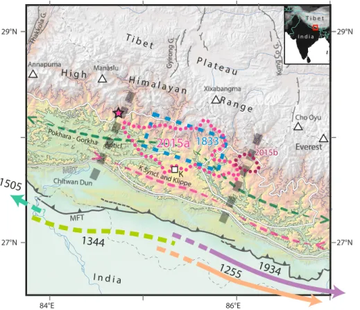
Figure 1. Tectonic and paleoseismological background of the 2015 Gorkha earthquake. Thick dashed arrows indicate lateral extension of surface rupture of past great earthquakes. Location of the 1833 earthquake (in blue) is from Bollinger et al. [2015]. The pink and brown dotted lines show the area of significant slip (>2 m) of the 25 April 2015 Gorkha earth-quake main shock and the 12 May 2015 aftershock, respectively (this study). Epicenter of the main shock reported by NSC is indicated by the pink star. Green and purple dashed lines show the location and along-strike tapering of the Pokhara-Gorkha anticline and Kathmandu synclinal, respectively. Thick grey lines delimit the inferred Kathmandu segment. The 1000 m and 3000 m elevation contours are represented by thin black lines. White triangles indicate peaks with elevation higher than 8000 m. Normal faults are indicated by grey barbed lines. MFT, Main Frontal Thrust; MBT, Main Boundary Thrust; MCT, Main Central Thrust; and K, Kathmandu.

SAR data are complemented by static offsets of the Nepal GPS Geodetic Network. Nine stations located less than 200 km from the epicenter are considered in this study (Figures 2a and 3a).

Local ground motion data includefive GPS stations from the same network, processed at high rate (5 Hz), complemented with the KATNP accelerometer in Kathmandu (Figure 2a). Near-fault displacement records

Figure 2. Rupture process of the Gorkha earthquake. (a) Slip distribution with 2 m slip contours. Grey dashed line deline-ates the surface projection of the modeled fault. Grey arrows show the direction of slip. Yellow symbols are back projection peaks, with their size proportional to the relative stack power. Grey circles are M> 4.5 aftershocks reported by Adhikari et al. [2015] until 8 June 2015. White star is NSC hypocenter. White square indicates location of Kathmandu city. Red symbols show the location of the closest stations used in this study. Slip model of the 12 May aftershock constrained by inversion of InSAR data (Figure S8) is indicated by a dashed contour. (b) Snapshots of slip distribution as a function of time deduced from kinematic inversion. Squares and circles indicate location of back projection peaks for every time frame. (c) Observed and modeled surface displacement from ALOS-2 descending InSAR (left column) and Sentinel-1 ascending range pixel tracking (right column). The black arrow indicates line-of-sight (LOS) direction. A positive sign indicates motion toward the satellite, whereas negative sign corresponds to motion away from the satellite. The bottom panels show transects across the observed and modeled surface displacementfields at locations shown by the grey lines in the maps. (d) Back projection (BP) peaks (1.0–4.0 Hz) superimposed on isochrones of kinematic inversion relative to hypocentral time. The dashed line shows the 2 m slip contour. (e) Source time function (STF) from kinematic inversion.

(KKN4, NAST, and KATNP) and farther ones (RMTE, SNDL, and SYBC) are low-passfiltered at 0.1 Hz and 0.05 Hz, respectively, in order to account for the increasing inaccuracy of wave modeling with distance. A high-passfilter of 0.015 Hz and 0.01 Hz is applied to the KATNP displacement records and to the high-rate GPS data, respectively. Wefinally add the teleseismic body wave P and SH records to this data set, for their ability to resolve the global temporal evolution of the earthquake. We use broadband signals from the Federation of Digital Seismograph Networks, with an azimuthal coverage avoiding locations where radiation pattern predicts low amplitude waves. Both P and SH displacement waveforms are band-passfiltered between 0.005 Hz and 0.125 Hz. This geodetic and seismic data set is simultaneously inverted using the method of Delouis et al. [2002]. The model consists of a single fault segment, 153 km long and 72 km wide, subdivided into 136 subfaults measuring 9 km along strike and dip, evenly distributed on the fault plane. The geometry of the fault is held fixed, controlled by its strike and dip angles (strike = 285°, dip = 7°), the epicentral location (84.75°E, 28.24°N) provided by NSC (Nepal National Seismological Centre) and a hypocentral depth of 16 km. These values have been previously optimized by a careful analysis of independent data types. In particular, the shallow dip is required both by SAR and teleseismic data and is in agreement with global analyses (e.g., GCMT, Ekström et al. [2012] and SCARDEC, Vallée et al. [2011]). As for depth determination, when the rupture approaches the surface, teleseismic data require increasingly more seismic moment, while SAR data require increasingly less slip. As a consequence, shallower or deeper depths lead to discrepancies between teleseismic and SAR data.

To model the waveforms, the continuous rupture is approximated by a summation of point sources at the center of each subfault. For each point source, the local source time function is represented by two mutually overlapping isosceles triangular functions of duration equal to 6 s. For each of the 136 subfaults, the parameters to be inverted are the slip onset time, the rake angle, and the amplitudes of the two triangular functions. A nonlinear inversion is performed using a simulated annealing optimization algorithm. Convergence criterion is based on the minimization of the root-mean-square data misfit, with optional smoothing constraints on the coseismic slip, rupture velocity, and rake angle variations, used in order to penalize unnecessarily complex models. In particular, the smoothing constraint on the rupture velocity is implemented by penalizing models with large variations of the average rupture velocity (from the hypocenter to the considered subfault) between adjacent subfaults.

All synthetic data (seismograms and static offsets) are computed in the same stratified crustal model (Table S2). This model takes into account the deep Moho in northern Nepal (48 km) and the relatively low P wave velocities (5.6 km/s) at shallow depth indicated by several studies [e.g., Monsalve et al., 2006]. Results in terms of coseismic

Figure 3. Comparison of observed and modeled (a) GPS displacements, (b) high-rate GPS and accelerometric records, and (c) teleseismic records. In the three sub_{figures, data are in black and synthetics in red. In Figure 3c, the text shown for each seismogram has the format: name of the station, type of the wave,} maximum amplitude in microns, and azimuth to the north in degrees.

slip vary marginally if using other crustal models due to the strong control provided by SAR data. Local synthetic seismograms (HRGPS and accelerometric data) and teleseismic P and SH displacements are computed using the discrete wave number method of Bouchon [1981] and the reciprocity approach of Bouchon [1976], respec-tively. Static displacements (for static GPS and SAR) are computed using the static Green functions approach of Wang et al. [2003].

2.2. High-Frequency Source Emissions From Teleseismic Back Projection

The spatiotemporal history of high-frequency (HF) source emissions is determined by back projection of teleseismic P waves recorded at the Virtual European Broadband Seismic Network (VEBSN) [van Eck et al., 2004], at stations in Australia and Southeast Asia, and in Alaska (Figures 2d and S1). P wave velocity records arefiltered between 1.0 and 4.0 Hz and back projected over a source grid of 350 km along strike and 200 km along dip, with an interval of 5 km. Theoretical travel times are computed using a 1-D global velocity model [Kennett et al., 1995]. Station corrections, accounting for deviations from the 1-D model, are calculated by cross correlation of thefirst-arrival P waveforms, preliminary aligned according to the NSC hypocenter. For each grid node, we compute a normalized trace stack weighted by semblance [Vallée et al., 2008], and we search for peaks of the stack power, in space and time, using a local maximumfilter (Figures S1 and S2). Finally, back projection peak times are corrected for the directivity effect, computed as the difference between the P wave travel time from the given peak and the travel time from the hypocenter (for an average station location). More details on the back projection technique, which is related to the methods of Xu et al. [2009] and Ishii et al. [2005], can be found in Satriano et al. [2012] and Vallée and Satriano [2014].

2.3. Interseismic Strain Accumulation

We also use surface displacement measurements acquired before the earthquake to quantify the spatial dis-tribution of interseismic coupling on the plate interface (Figures S3 and S4). We update the solution of Grandin et al. [2012] by modeling deformation using a back slip approach with a dislocation embedded in an elastic half-space with depth-dependent rigidity [Vergne et al., 2001]. The fault has a constant dip of 7° and coincides with the 2015 coseismic fault. Its strike varies smoothly so as to follow the trace of the MFT. The interface is divided into 32 km (along-strike) by 10 km (along-dip) rectangular patches. Smoothing is achieved by Laplacian constraints introduced in the model covariance matrix. The smoothing intensity is controlled by a metaparameter whose value is adjusted by an L curve criterion approach. Bounds on the convergence rate between 0 and 18 mm/yr are implemented by means of sequential quadratic program-ming. Rake isfixed so that the azimuth of convergence is everywhere N10°E. The horizontal components of surface displacement are constrained using a compilation of GPS data from Bettinelli et al. [2006], Feldl and Bilham [2006], Socquet et al. [2006], Gan et al. [2007], Banerjee et al. [2008], and Ader et al. [2012]. Leveling data from Jackson and Bilham [1994] for the period 1977–1990 are also used for the vertical component.

3. Results and Discussion

3.1. Rupture Process and Relations With Strong Motion Generation

The source process shown in Figure 2 corresponds to a kinematic fault slip inversion giving similar weights to the four data types (SAR, GPS, local waveforms, and teleseismic data), with small smoothing constraints on slip amplitude, rupture velocity, and rake angle. Rupture velocity is here constrained to be between 2.1 km/s and 3.3 km/s (see Figure S5). As illustrated in the supporting information (Figures S6 and S7), the retrieved source process is essentially the same when allowing for a wider range of possible rupture velocity and for a full relaxa-tion of slip and rupture velocity smoothing constraints. The kinematic fault slip inversion and back projecrelaxa-tion reveal that the rupture propagated unilaterally from west to east over a distance of 120 km (Figure 2a). Spatiotemporal distributions of coseismic slip and back projection peaks are in good agreement, at a time resolution of 10 s (Figures 2b and 2d). At smaller time scales, the effect of crust-reflected phases (pP and sP) can affect the relative timing of back projection peaks [Okuwaki et al., 2014; Yagi and Okuwaki, 2015], with however, only minor distortion of the relative peak location as discussed, for instance, in Fan and Shearer [2015]. The obtained source time function (Figure 2e) shows that the total duration of the earthquake is close to 50 s, and its seismic moment is 7.7 × 1020N m (Mw= 7.86). The rupture history shown in Figure 2b is in good

agreement with all the data used in the kinematic inversion (Figures 2c and 3c). The dominant feature of the slip model is a 13–15 km deep patch (slip larger than 4 m and reaching 7 m) whose rupture starts 10 s after

earthquake initiation, 25 km southeast of the epicenter. This patch has a size of about 80 km along strike and 25 km along dip, an elongated aspect ratio very well constrained by the SAR data (Figure 2c). Aftershocks delineate the contours of this patch (Figure 2a), as a result of static stress transfer induced by the maximum slip gradients [e.g., Rietbrock et al., 2012]. Dynamic stress transfer can explain the larger number of aftershocks at the eastern termination of the rupture, as this area has experienced more dynamic stress due to the eastward rupture propagation. This area ruptured again on 12 May 2015 with an earthquake of Mw7.3 (Figure S8), which

was itself followed by an abundant aftershock sequence.

Rupture speed inside the main slip patch is well constrained by seismic data, and in particular by the three records close to Kathmandu (KATNP, KNAS, and KKN4, see Figure 3b), and is stable around 3.1–3.3 km/s (Figures 2b, S5, and S7). Thisfinding is confirmed by back projection analysis. Inside this patch, the rake shows only small variations, with values ranging between 90° and 100° (Figure 2a). This simple rupture process (single patch breaking with the same mechanism at constant rupture velocity) is a feature which is little affected by the band-limited frequencies used in the inversion, as illustrated by the good waveform agree-ment at station KKN4 for frequencies up to 1 Hz (Figure S9). Together with the fact that no high-frequency emission is recorded in the updip part of the rupture from back projection, this indicates that the rupture process was smooth as it passed North of Kathmandu and likely explains the relatively low peak ground acceleration (PGA) recorded in the capital (KATNP site, located only 20 km from the high slip patch, recorded a PGA of only 0.2 g, a value well below ground motion predictions) [Goda et al., 2015; Galetzka et al., 2015]. Indeed, abrupt changes of rupture velocity are theoretically known [Madariaga, 1977; Campillo, 1983; Sato, 1994] and have been observed [Vallée et al., 2008] to be the main origin of high-frequency radiations. The smooth character of the main patch rupture is also in good agreement with the study of Denolle et al. [2015], indicating that the fall-off rate of the P teleseismic spectrum increases 15 s after rupture initiation.

3.2. The Gorkha Earthquake in the Context of the Himalayan Collision Zone

Slip distribution of the 2015 Gorkha earthquake is imaged to spread over an area of 120 × 35 km parallel to the main trend of the mountain range (~N110°E) at a depth of ~15 km (Figure 2). The earthquake appears to have broken a portion of the MHT where coupling decreases from 100% (updip edge of the coseismic patch) to less than 25% (downdip edge) in less than 50 km (Figures 4, S3, and S4). This coupling gradient is highlighted by a belt of earthquakes that spatially follows the front of the High Himalayan range, at a depth of ~15 km. This seismic belt likely reflects stress concentration around the transition to deep stable sliding [e.g., Bilham et al., 2001; Bollinger et al., 2004a]. Coseismic slip shows a rapid decrease in the downdip direc-tion, consistent with the decreasing coupling limiting the propagation of the rupture to greater depths. The downdip edge of the rupture zone also coincides spatially with locations of high-frequency emission (Figure 2a), as also evidenced by Yagi and Okuwaki [2015] and by Fan and Shearer [2015]. These observations suggest strong similarities with the behavior of megathrust earthquakes, where high-frequency radiations originate from the base of the seismogenic domain [Lay et al., 2012]. This feature is interpreted as a possible effect of the variability with depth of frictional and stress heterogeneity along the fault interface. The particularity of this transition zone in the Himalaya is its coincidence with the inferred junction between the frontalflat and a deeper ramp dipping at a steeper angle [Cattin and Avouac, 2000] (Figure 4b). As the feedbacks between geometry and seismic potential of the interface are difficult to ascertain, this coincidence may equally point to either a geometric-structural and/or to a thermal-rheological control as the underlying cause of the coupling gradient at the scale of a seismic cycle.

In contrast, the updip limit of coseismic slip cannot be readily interpreted in terms of a local decrease of the coupling ratio, as argued elsewhere to justify the arrest of large subduction earthquakes and ultimately the segmentation of seismicity [e.g., Métois et al., 2012]. On the contrary, coupling appears to be maximal to the south of the main slip patch, up to the MFT (Figure 4a). A similar situation has been observed in the case of the 2007 Tocopilla earthquake (Chile), which has occurred along the downdip limit of a highly coupled segment of the Chile megathrust. Structural complexity within the overriding plate was invoked as a factor contributing to the updip arrest of the 2007 Tocopilla rupture [Béjar-Pizarro et al., 2010] and, more widely, to the geometry of the transition zone and segmentation of the Chile megathrust [Béjar-Pizarro et al., 2013; Armijo et al., 2015]. In Nepal, the updip limit of the 2015 rupture zone broadly corresponds, in map view, with the southern limit of the antiform of Lesser Himalayan units observed all along Central Nepal Himalaya (Figure 1). This antiform is generally interpreted as resulting from stacking up of slices of upper crustal

material of Indian affinity involving several generations of ramps and flats [e.g., Schelling and Arita, 1991; Bollinger et al., 2004b; Khanal and Robinson, 2013]. If correct, this accretionary model has given rise to a complex geometry of the MHT at the location of the 2015 Gorkha earthquake. This along-dip structural complexity may have played a role in impeding the propagation of the coseismic rupture toward the surface. In the same line, lateral (east and west) limits of the coseismic slip are at odds with thefirst-order along-strike uniformity of interseismic strain accumulation in Central Nepal. In map view, the MHT appears to be fully locked between the High Himalayan Range and the trace of the MFT, approximately 100 km to the south (Figure 4a). We note that the absence of large lateral variations in interseismic coupling cannot be explained by insufficient spatial sampling of GPS stations [Ader et al., 2012]. Alternatively, the along-strike extension of the 2015 earthquake broadly matches with a section exhibiting a relatively uniform structural surface

Figure 4. (a) Interseismic coupling distribution on the Main Himalayan Thrust (MHT) deduced from GPS (green circles) and leveling (white circles) (this study). Slip contours of the 2015 Gorkha earthquake (25 April) and its main aftershock (12 May) are indicated by pink and brown lines, respectively (this study). The NSC hypocenter of the main shock is shown by the pink star. Blue circles show the seismicity recorded by the Nepalese network for the period 1995–2003 [Rajaure et al., 2013]. (b) Superimposition of interseismic coupling model and seismicity (dashed black box in Figure 4a) and geological cross section of Bollinger et al. [2004b] (transect A-A′). Pink arrow indicates along-dip extension of the 2015 Gorkha earthquake (this study). Histograms show distribution of 1995–2003 seismicity.

expression between 84.5°E and 86.0°E (Figure 1). This section, which we refer to as the“Kathmandu segment,” is characterized by (1) a narrower Lesser Himalayan antiform with its culmination (green dashed line in Figure 1) located further toward the hinterland compared to other sections in Central Nepal, as attested by a northerly trace of the Main Central Thrust (MCT), (2) a better preservation of the Higher Himalaya crystalline nappe, forming the broad Kathmandu klippe, and (3) a rather uniform parallelism of the MFT and Main Boundary Thrust (MBT), terminated by MBT reentrants at segment extremities. These features are likely indi-cative of lateral variations in the steepness, depth, and/or stacking history of the MHT in the area.

Ultimately, the origin of these lateral variations may be partly attributed to lateral sweeping of the interface as heterogeneities within the upper crustal cover of the Indian plate, such as ridges or troughs in the Ganga Basin, are underthrusted below the MHT [Bollinger et al., 2004b ; Denolle et al., 2015]. Modifications of the MHT geometry imparted by such variations in boundary conditions can be relatively immediate. However, the geomorphological expression of these modifications can be delayed due to the comparatively long response time of erosion processes, so that correlating the geological record and instantaneous deformation may not be straightforward [Grandin et al., 2012].

3.3. Implications for Seismic Hazards

The Gorkha earthquake not only provides a direct confirmation of the seismogenic potential of the MHT but also illustrates the great difficulty in anticipating along-dip and along-strike limits of future megathrust earth-quakes based solely on the mapping of interseismic coupling. Even so, afirst-order conclusion that can be drawn from the size and location of the 2015 Gorkha event is its failure to release a significant fraction of the tectonic strain previously accumulated within the MHT system in the broad Kathmandu area. With an average slip of ~4 m, the earthquake has only accommodated approximately 200 years of local slip accumu-lation. The 2015 blind rupture could therefore be interpreted as the repetition of the 1833 earthquake [Bollinger et al., 2015] (Figure 1). However, the frontal part of the MHT, which was not activated by the earth-quake, appeared to be fully locked before the event (Figure 4). The previous great earthquake in the area dates back to at least 1505 and probably to 1344, which represents more than 10 m of slip accumulation. The updip arrest of the 2015 rupture does not preclude a seismogenic potential of the MHT at shallow depth, as exemplified by the updip progression of the earthquake sequence in the Mejillones Peninsula area, in Chile, with a relatively deep M7.5 earthquake in 1987 followed by the shallower M8.1 Antofagasta earthquake in 1995 [Delouis et al., 1997].

Actually, static stress transfer induced by the 2015 Gorkha earthquake can only add to this worrying situation. It is currently impossible to exclude that the slip deficit remaining at shallow depths will be filled by contin-uous creep of the interface or by a relatively low frequency, potentially less destructive continental analogue of the so-called tsunami earthquakes described in subduction settings [Lay et al., 2012]. Continued geodetic monitoring of the area in the coming years will provide a quantitative answer to these speculations. Nevertheless, except for the unlikely detection of a massive afterslip event taking place within the shallow part of the MHT, it is currently unsafe to discard a scenario whereby the frontal part of the megathrust will rupture during a great earthquake in the future. This scenario would be entirely in keeping with the conclu-sions previously drawn from geodetic, paleoseismological, and historical inferences [e.g., Bilham et al., 2001]. Finally, even if only a fraction of the gap south of the 2015 rupture zone breaks in a future earthquake— resulting in an earthquake in the Mw7–8 magnitude range—a realistic scenario with a rupture closer to

Kathmandu and involving more high-frequency emissions might still affect the city in a stronger way than the 2015 Gorkha earthquake.

References

Ader, T., et al. (2012), Convergence rate across the Nepal Himalaya and interseismic coupling on the Main Himalayan Thrust: Implications for seismic hazard, J. Geophys. Res., 117, B04403, doi:10.1029/2011JB009071.

Adhikari, L. B., et al. (2015), The aftershock sequence of the April 25 2015 Gorkha-Nepal earthquake, Geophys. J. Int. (accepted). Armijo, R., R. Lacassin, A. Coudurier-Curveur, and D. Carrizo (2015), Coupled tectonic evolution of Andean orogeny and global climate, Earth

Sci. Rev., 143, 1–35.

Avouac, J. P., and P. Tapponnier (1993), Kinematic model of active deformation in Central Asia, Geophys. Res. Lett., 20(10), 895–898, doi:10.1029/93GL00128.

Banerjee, P., R. Bürgmann, B. Nagarajan, and E. Apel (2008), Intraplate deformation of the Indian subcontinent, Geophys. Res. Lett., 35, L18301, doi:10.1029/2008GL035468.

Acknowledgments

GPS data from the Nepal GPS Geodetic Network were taken from UNAVCO website. GPS processing was performed as part of the ARIA project, using GIPSY-OASIS software and JPL Rapid and Final orbits and clock products. ARIA is supported by NASA and NSF. We thank Jean-Philippe Avouac, Jeff Genrich, and John Galetzka for making these results available. We thank the Nepal Government, Department of Mines and Geology and National Seismological Centre (NSC), for sharing the aftershock catalog at http://www.seismonepal.gov. np. We thank ESA for quickly responding to Sentinel-1 acquisition requests. Sentinel-1 data were processed using ROI_PAC [Rosen et al., 2004]. We are grateful to the USGS NetQuakes service for free access to the data of the KATNP station and to the global broadband seismic networks (IRIS and GEOSCOPE) for free access to their high-quality broadband seismic data. We are grateful to broadband seismic network operators (AK, AT, AU, AV, BS, BW, CA, CH, CN, CZ, DK, EE, EI, FN, G, GB, GE, GR, GU, HE, HL, HT, HU, II, IU, IV, MD, MN, MY, NI, NO, OE, PL, PM, RM, RO, S, SJ, SL, SS, SX, TA, TH, TT, TU, US, WM), for high-quality data and public access to continuous waveforms. VEBSN data were retrieved through the European Integrated Data Archive (EIDA) web portal (www.orfeus-eu.org/eida). Data for Australia/Southeast Asia and Alaska were retrieved through the Incorporated Research Institutions for Seismology (IRIS) Wilber 3 service (http:// ds.iris.edu/wilber3). R.G. thanks Romain Jolivet for providing assistance with the inversion code CSI. M.V. thanks Bertrand Delouis for sharing his rupture inversion program. Some numerical computations were performed on the S-CAPAD platform, IPGP, France. This is IPGP contribution 3680. This project was supported by PNTS grant“PNTS-2015-09” and by the“BHUTANEPAL” project funded by the Agence Nationale de la Recherche (ANR). The authors thank two anonymous reviewers for their comments that helped improve the manuscript.

Béjar-Pizarro, M., et al. (2010), Asperities and barriers on the seismogenic zone in North Chile: State-of-the-art after the 2007 Mw7.7 Tocopilla

earthquake inferred by GPS and InSAR data, Geophys. J. Int., 183(1), 390–406.

Béjar-Pizarro, M., A. Socquet, R. Armijo, D. Carrizo, J. Genrich, and M. Simons (2013), Andean structural control on interseismic coupling in the North Chile subduction zone, Nat. Geosci., 6(6), 462–467.

Bettinelli, P., J. P. Avouac, M. Flouzat, F. Jouanne, L. Bollinger, P. Willis, and G. R. Chitrakar (2006), Plate motion of India and interseismic strain in the Nepal Himalaya from GPS and DORIS measurements, J. Geod., 80(8–11), 567–589.

Bilham, R., V. K. Gaur, and P. Molnar (2001), Himalayan seismic hazard, Science, 293(5534), 1442–1444.

Bollinger, L., J. P. Avouac, R. Cattin, and M. R. Pandey (2004a), Stress buildup in the Himalaya, J. Geophys. Res., 109, B11405, doi:10.1029/ 2003JB002911.

Bollinger, L., et al. (2004b), Thermal structure and exhumation history of the Lesser Himalaya in central Nepal, Tectonics, 23, TC5015, doi:10.1029/2003TC001564.

Bollinger, L., P. Tapponnier, S. N. Sapkota, and Y. Klinger (2015), Slip deficit in central Nepal: Omen for a pending repeat of the 1344 AD earthquake?, under revision for Nat. Commun.

Bouchon, M. (1976), Teleseismic body wave radiation from a seismic source in a layered medium, Geophys. J. Int., 47, 515–530. Bouchon, M. (1981), A simple method to calculate Green’s functions for elastic layered media, Bull. Seismol. Soc. Am., 71, 959–971. Campillo, M. (1983), Numerical evaluation of the near-field high-frequency radiation from quasidynamic circular faults, Bull. Seismol. Soc. Am.,

73, 723–734.

Cattin, R., and J. P. Avouac (2000), Modeling mountain building and the seismic cycle in the Himalaya of Nepal, J. Geophys. Res., 105(B6), 13,389–13,407, doi:10.1029/2000JB900032.

Delouis, B., et al. (1997), The Mw= 8.0 Antofagasta (northern Chile) earthquake of 30 July 1995: A precursor to the end of the large 1877 gap,

Bull. Seismol. Soc. Am., 87, 427–445.

Delouis, B., D. Giardini, P. Lundgren, and J. Salichon (2002), Joint inversion of InSAR, GPS, teleseismic, and strong-motion data for the spatial and temporal distribution of earthquake slip: Application to the 1999 Izmit mainshock, Bull. Seismol. Soc. Am., 92, 278–299.

Denolle, M. A., W. Fan, and P. M. Shearer (2015), Dynamics of the 2015 M7.8 Nepal earthquake, Geophys. Res. Lett., 42, doi:10.1002/ 2015GL065336.

Ekström, G., M. Nettles, and A. M. Dziewonski (2012), The global CMT project 2004–2010: Centroid-moment tensors for 13,017 earthquakes, Phys. Earth Planet. Inter., 200–201, 1–9.

Fan, W., and P. M. Shearer (2015), Detailed rupture imaging of the 25 April 2015 Nepal earthquake using teleseismic P waves, Geophys. Res. Lett., 42, 5744–5752, doi:10.1002/2015GL064587.

Feldl, N., and R. Bilham (2006), Great Himalayan earthquakes and the Tibetan plateau, Nature, 444(7116), 165–170.

Galetzka, J., et al. (2015), Slip pulse and resonance of Kathmandu basin during the 2015 Mw7.8 Gorkha earthquake, Nepal imaged with

geodesy, Science, doi:10.1126/science.aac6383.

Gan, W., et al. (2007). Present-day crustal motion within the Tibetan Plateau inferred from GPS measurements, J. Geophys. Res., 112, B08416, doi:10.1029/2005JB004120.

Goda, K., T. Kiyota, R. M. Pokhrel, G. Chiaro, T. Katagiri, K. Sharma, and S. Wilkinson (2015), The 2015 Gorkha Nepal earthquake: Insights from earthquake damage survey, Front. Built Environ., 1, 8, doi:10.3389/fbuil.2015.00008.

Grandin R. (2015), Interferometric Processing of SLC Sentinel-1 TOPS Data, Proceedings of the 2015 ESA Fringe workshop, ESA Special Publication, SP-731, Frascati, Italy.

Grandin, R., M. P. Doin, L. Bollinger, B. Pinel-Puysségur, G. Ducret, R. Jolivet, and S. N. Sapkota (2012), Long-term growth of the Himalaya inferred from interseismic InSAR measurement, Geology, 40(12), 1059–1062.

Herman, F., et al. (2010), Exhumation, crustal deformation, and thermal structure of the Nepal Himalaya derived from the inversion of thermochronological and thermobarometric data and modeling of the topography, J. Geophys. Res., 115, B06407, doi:10.1029/ 2008JB006126.

Ishii, M., P. M. Shearer, H. Houston, and J. E. Vidale (2005), Extent, duration and speed of the 2004 Sumatra-Andaman earthquake imaged by the Hi-Net array, Nature, 435, 933–936, doi:10.1038/nature03675.

Jackson, M., and R. Bilham (1994), Constraints on Himalayan deformation inferred from vertical velocityfields in Nepal and Tibet, J. Geophys. Res., 99(B7), 13,897–13,912, doi:10.1029/94JB00714.

Kennett, B., E. R. Engdahl, and R. Buland (1995), Constraints on seismic velocities in the Earth from traveltimes, Geophys. J. Int., 122(1), 108–124, doi:10.1111/j.1365-246X.1995.tb03540.x.

Khanal, S., and D. M. Robinson (2013), Upper crustal shortening and forward modeling of the Himalayan thrust belt along the Budhi-Gandaki River, central Nepal, Int. J. Earth Sci., 102(7), 1871–1891.

Lavé, J., and J. P. Avouac (2000), Active folding offluvial terraces across the Siwaliks Hills, Himalayas of central Nepal, J. Geophys. Res., 105(B3), 5735–5770, doi:10.1029/1999JB900292.

Lay, T., et al. (2012), Depth-varying rupture properties of subduction zone megathrust faults, J. Geophys. Res., 117, B04311, doi:10.1029/ 2011JB009133.

Lindsey, E., R. Natsuaki, X. Xu, M. Shimada, H. Hashimoto, D. Melgar, and D. Sandwell (2015), Line of sight deformation from ALOS-2 interferometry: Mw7.8 Gorkha earthquake and Mw7.3 aftershock, Geophys. Res. Lett., 42, 6655–6661, doi:10.1002/2015GL065385.

Madariaga, R. (1977), High-frequency radiation from crack (stress drop) models of earthquake faulting, Geophys. J. Int., 51, 625–651. Métois, M., A. Socquet, and C. Vigny (2012), Interseismic coupling, segmentation and mechanical behavior of the central Chile subduction

zone, J. Geophys. Res., 117, B03406, doi:10.1029/2011JB008736.

Monsalve, G., A. Sheehan, V. Schulte-Pelkum, S. Rajaure, M. R. Pandey, and F. Wu (2006), Seismicity and one-dimensional velocity structure of the Himalayan collision zone: Earthquakes in the crust and upper mantle, J. Geophys. Res., 111, B10301, doi:10.1029/2005JB004062. Okuwaki, R., Y. Yagi, and S. Hirano (2014), Relationship between high-frequency radiation and asperity ruptures, revealed by hybrid

back-projection with a non-planar fault model, Sci. Rep., 4, 7120, doi:10.1038/srep07120.

Rajaure, S., et al. (2013), Double difference relocation of local earthquakes in the Nepal Himalaya, J. Nepal Geol. Soc., 40, 133–142. Rietbrock, A., I. Ryder, G. Hayes, C. Haberland, D. Comte, S. Roecker, and H. Lyon-Caen (2012), Aftershock seismicity of the 2010 Maule Mw= 8.8,

Chile, earthquake: Correlation between co-seismic slip models and aftershock distribution? Geophys. Res. Lett., 39, L08310, doi:10.1029/2012GL051308.

Rosen, P. A., S. Hensley, G. Peltzer, and M. Simons (2004), Updated repeat orbit interferometry package released, Eos Trans. AGU, 85(5), 47–47, doi:10.1029/2004EO050004.

Sapkota, S. N., L. Bollinger, Y. Klinger, P. Tapponnier, Y. Gaudemer, and D. Tiwari (2013), Primary surface ruptures of the great Himalayan earthquakes in 1934 and 1255, Nat. Geosci., 6(1), 71–76.

Sato, T. (1994), Seismic radiation from circular cracks growing at variable rupture velocity, Bull. Seismol. Soc. Am., 84, 1199–1215. Satriano, C., E. Kiraly, P. Bernard, and J. P. Vilotte (2012), The 2012 Mw8.6 Sumatra earthquake: Evidence of westward sequential seismic

ruptures associated to the reactivation of a N-S ocean fabric, Geophys. Res. Lett., 39, L15302, doi:10.1029/2012GL052387.

Schelling, D., and K. Arita (1991), Thrust tectonics, crustal shortening, and the structure of the far-eastern Nepal Himalaya, Tectonics, 10(5), 851–862, doi:10.1029/91TC01011.

Socquet, A., C. Vigny, N. Chamot-Rooke, W. Simons, C. Rangin, and B. Ambrosius (2006), India and Sunda plates motion and deformation along their boundary in Myanmar determined by GPS, J. Geophys. Res., 111, B05406, doi:10.1029/2005JB003877.

Szeliga, W., S. Hough, S. Martin, and R. Bilham (2010), Intensity, magnitude, location, and attenuation in India for felt earthquakes since 1762, Bull. Seismol. Soc. Am., 100(2), 570–584.

Vallée, M., and C. Satriano (2014), Ten year recurrence time between two major earthquakes affecting the same fault segment, Geophys. Res. Lett., 41, 2312–2318, doi:10.1002/2014GL059465.

Vallée, M., M. Landès, N. M. Shapiro, and Y. Klinger (2008), The 14 November 2001 Kokoxili (Tibet) earthquake: High-frequency seismic radiation originating from the transitions between sub-Rayleigh and supershear rupture velocity regimes, J. Geophys. Res., 113, B07305, doi:10.1029/2007JB005520.

Vallée, M., J. Charléty, A. M. G. Ferreira, B. Delouis, and J. Vergoz (2011), SCARDEC: A new technique for the rapid determination of seismic moment magnitude, focal mechanism and source time functions for large earthquakes using body wave deconvolution, Geophys. J. Int., 184, 338–358.

van Eck, T., C. Trabant, B. Dost, W. Hanka, and D. Giardini (2004), Setting up a virtual broadband seismograph network across Europe, Eos Trans. AGU, 85(13), 125, doi:10.1029/2004EO130001.

Vergne, J., R. Cattin, and J. P. Avouac (2001), On the use of dislocations to model interseismic strain and stress build-up at intracontinental thrust faults, Geophys. J. Int., 147(1), 155–162.

Wang, R., F. Lorenzo-Martin, and F. Roth (2003), Computation of deformation induced by earthquakes in a multi-layered elastic crust—FORTRAN programs EDGRN/EDCMP, Comput. Geosci., 29(2), 195–207.

Xu, Y., K. D. Koper, O. Sufri, L. Zhu, and A. R. Hutko (2009), Rupture imaging of the Mw7.9 12 May 2008 Wenchuan earthquake from back

projection of teleseismic P waves, Geochem. Geophys. Geosyst., 10, Q04006, doi:10.1029/2008GC002335.

Yagi, Y., and R. Okuwaki (2015), Integrated seismic source model of the 2015 Gorkha, Nepal, earthquake, Geophys. Res. Lett., 42, 6229–6235, doi:10.1002/2015GL064995.