Cortical sulci model and matching from 3D brain magnetic resonance images

HAL Id: hal-00963684

https://hal.archives-ouvertes.fr/hal-00963684

Submitted on 21 Mar 2014

HAL is a multi-disciplinary open access archive for the deposit and dissemination of sci-entific research documents, whether they are pub-lished or not. The documents may come from teaching and research institutions in France or abroad, or from public or private research centers.

L’archive ouverte pluridisciplinaire HAL, est destinée au dépôt et à la diffusion de documents scientifiques de niveau recherche, publiés ou non, émanant des établissements d’enseignement et de recherche français ou étrangers, des laboratoires publics ou privés.

Cortical sulci model and matching from 3D brain

magnetic resonance images

Serge Langlois, Nicolas Royackkers, Houssam Fawal, Michel Desvignes,

Marinette Revenu, Jean-Marcel Travère

To cite this version:

Serge Langlois, Nicolas Royackkers, Houssam Fawal, Michel Desvignes, Marinette Revenu, et al.. Cortical sulci model and matching from 3D brain magnetic resonance images. 5st Int. Conf. on Image Processing and its applications, 1995, Edinburgh, United Kingdom. pp.124-128. �hal-00963684�

CORTICAL SULCI MODEL AND MATCHING FROM 3D BRAIN MAGNETIC RESONANCE IMAGES

S Langlois(1), N Royackkers(1), H Fawal(1), M Desvignes(1), M Revenu(1), J M Travere(2).

(1)

GREYC-ISMRA, France (2) CYCERON, France

INTRODUCTION

Positron Emission Tomography (PET) is one of the most popular technique for the study of brain functional activity. Several studies as in Fox et al (1), Neelin et al (2) show that PET is an in-vivo examination technique able to produce real images of cerebral activity, and is also neither destructive nor invasive. Unfortunately, PET images offer low resolution and signal-to-noise ratio. Moreover, they do not reflect the anatomy of patients. Accurate and reproducible analysis of PET images requires other informations, coming from atlases or other images such as Magnetic Resonance Image (MRI) of the same patient (Evans et al (3)). According to Rademacher et al (4), MRI offers accurate in-vivo localisation of anatomical landmarks. It has been used to estimate individual variations and left-right asymmetries of sulci and gyri. Hence, it is of great interest to superimpose functional PET data and anatomical MRI data.

One approach to this problem is to use the stereotactic proportional grid of Talairach and Tournoux (5). It defines spatial co-ordinates of brain sulci and gyri, and of cytoarchitectonic fields. Despite the application of scaling factors, the accuracy of standard brain atlas superimposition onto any given examination is about one to two centimetres at the cortical level, because of inter-individual variations described in Greitz et al (6). Another approach, used by Jouandet et al (7), determines cortical maps based on the topography of sulci and gyri. Our work is based on this method and our objective is to automatically recognise cortical sulci of any brain MRI examination, with respect to an anatomical atlas. Individual recognition of those structures is relevant to the general problems of image registration and search for a set of objects among a set of reference. It can be summarised by looking for the largest common structure in two different graphs, and can be performed using several methods as templates and springs described in Ballard and Braun (8), maximal cliques in Miclet (9), tree search in Vausselman (10) or relaxation techniques in Hummel and Zucker (11). The main problem is the large variation of dimensions and patterns of patients' brains and sulci. Classical features (length, orientation...) cannot be directly used to identify sulci and are very difficult to be determined. In this paper, we deal with representation and identification of sulci. A first step is to choose and to automatically extract anatomical knowledge from a database, in order to adapt it to any image where the

recognition has to be performed. Then, we introduce a stochastic method using these features to recognise human cerebral sulci.

DATA AND FEATURE EXTRACTION

In a previous work, Desvignes et al (12) have established a heuristic search based on spatial location and relations among neighbouring sulci. Localisation, global and local orientations, local depth (depth of sulcus from cortical surface) and continuity are the main features of one sulcus. Connections with other sulci are also necessary relations for sulci identification.

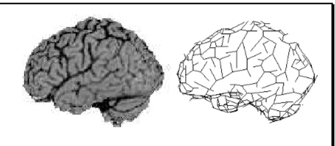
Data are issued from 3D MRI images (120x256x256 voxels, SPGR sequence, Signa 1.5T General Electrics Medical Systems unit). Brain is extracted and segmented into Cerebro Spinal Fluid (CSF), White Matter and Grey Matter as shown in Allain et al (13). Sulci are cerebral structures filled with CSF. 3D skeletonization and 3D curve thinning are applied to CSF. Sulci are then described by 3D digital curves on the cortical surface (Figure 1).

Six sulci have been identified on a training set of nine brains. For each sulci, principal axis, centre of gravity, middle point, continuity (number and position of parts), localisation and connections with others sulci are computed. For each point, depth of the sulci is computed using a tangent vector method. Localisation, orientation and pattern are described by a search window. All the sulci of the training set are superimposed to obtain a cloud of points. 3D morphological operators are used to obtain a compact zone (dilation, hole filling) and to smooth its edge (conditional dilation). A 3D conditional thinning algorithm transforms this search window into a graph of segments, which is a close approximation of the iconic drawing used in medical atlases (Figure 2).

Figure 1: Lateral projection of a MRI image (left), polygonal description of sulci (right)

Not all of these features are used during the matching process. At this stage, we introduce depths of sulci and search windows.

METHODS: RELAXATION PROCESS AND OPTIMISATION

Continuous relaxation (11) is an iterative algorithm which correspond to a probabilistic approach of graph matching. We applied this process to match a graph of segments coming from a brain image, with another examination where sulci have already been identified. Each assignment i→ I between elements i and I from two sets is referred to a real coefficient

p

_it

(I )

, that depends on all the coefficients

p

t_j−1

(J )

computed at the preceding step.

This process is based on the propagation, along the graphs, of constraints Rijk...(I,J,K...) that quantify the

similarity between two structures of nodes (i,j,k...) and (I,J,K...).

Li (14) explains that this technique offers the advantage of a global combinatorial solution, achieved through local propagation, which does not require any threshold to judge acceptance of individual matches .

Let n and N be the numbers of nodes from the two graphs to be matched, and r the number of nodes (i,j,k..) and (I,J,K..) considered in the constraints. The main characteristic of the relaxation process is its complexity in O(nr.Nr ). Hence, the polygonal description into segments allows the use of binary constraints Rij(I,J)

(equation IV), leading to a reduced CPU time.

Unfortunately, continuous relaxation describes a homomorphism from one set onto the other, that suffers from the ambiguous matching and 'Nil class' problems: if each segment from the set of objects has only one assignment in the set of labels, one label can be assigned to several objects or can remain unassigned.

During a relaxation process, a consistent labelling p , defined in Rosenfeld et al (15), is computed at each step t by maximising an average local consistency Gt( p ),

called the gain of relaxation (equation I).

G

t

( p) =

R

_ij

(IJ ).p

_it

(I ).p

t_j

(J )

J =1 N

∑

j =1 n

∑

I =1 N

∑

i =1 n

∑

(I)

This maximum gain is obtained by updating the assignments

p

i

t

(I )

according to a gradient ascent method, where each

p

_it

(I )

is moved towards the direction of this gradient (equations II and III).

p

i t+1

_{(I )}

=

p

i t

(I ) 1 + q

⎡⎣

_it

(I )

⎤⎦

p

i t

(I ) 1 + q

_it

(I )

⎡⎣

⎤⎦

(

)

I

∑

(II)

q

_it

(I ) =

J=1 N

∑

j=1 n

∑

R

_ij

(I, J ).p

t_j

(J )

(III) ( denominator of equation II insures that

p

i

t I=1

N

∑

(I )

=1 ) Update leads, in the ideal case, to an individual labelling assignment (pi( I ) = 1 and pi(J)=0 ∀ I

###

J),

corresponding to a constant gain Gt.

We now present a bi-relaxation method, which ensures a unique labelling, and is based on a relaxation algorithm where CPU time is reduced.

Optimisation

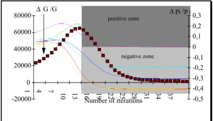
An experimental study (Figure 3) emphasises common properties from variations of the gain and variations of

p

i t

(I )

. We can notice that from the time where ΔGt/Gt (=1-Gt-1/Gt) comes up to a maximum value, each

Δ p

i t

(I ) / p

_it

(I )

reaches a limit with always the same sign. Starting from any value, since our objective is to determine every individual assignment, it thus becomes useless to expect a constant gain. Decreasing

p

_it

(I )

are deleted, while increasing ones are kept for the same

Figure 3: Relative variations of the gain G and of the probabilities pi versus number of iterations

-20000 0 20000 40000 60000 80000 1 4 7 _{10 13 16 19 22 25 28 31 34 37} -0,5 -0,4 -0,3 -0,2 -0,1 0 0,1 0,2 0,3 Number of iterations ΔG /G _Δp /p_{i i} positive zone negative zone

Figure 2: Conditional thinning algorithm applied on the lateral sulcus point cloud

process, starting again with a reduced number of segments. Individual labelling assignment is inevitably reached, through only a few iterations. Reduced CPU time then allows shape matching between sets of larger sizes in less time.

Bi-relaxation

Previous problems of ambiguous matching and 'Nil class' have been solved as in Legoupil et al (16). Two relaxation processes are applied, one from one set onto the other and conversely. The isomorphism defined allows assignments from each node of both two sets with at most one label, that is to say only one or none. The main principle of bi-relaxation is to apply a symmetrical processing of the two graphs, and to delete all the elements that do not respect the constraints. However, deletions require to achieve another bi-relaxation, in order to make sure that assignments are exactly the same as those obtained between the two initial sets (Figure 4). In the opposite case, the operation is iterated until no more suppressions are needed.

APPLICATION

3D MRI images of the head stem from clinical exams of sane patients. Each brain hemisphere is described by a graph where nodes are segments, and arcs are 3D geometrical relations between segments.

To apply relaxation process to sulci matching, we first have to define similarity functions, that map geometrical difference between two pairs of segments (i,j) and (I,J) from two sulci. Then these functions have to be weighted and combined in the constraint function Rij(IJ), so as to define their relative influence. Finally,

since the process is iterative, suitable initial values must be set for pi(I) and pI(i).

Similarity functions

Similarity functions required by the graph labelling process represent the main properties of sulci which are continuity and relative orientation of their segments. We selected the minimum distance between two segments, and a function representative of both the absolute angle defined by two segments i and j and the difference between the angles of two couples of segment (i,j) and (I,J).

Due to our two original sets defined in the same volume, it must be noticed that one of our similarity functions has to be dependant on scale changes.

Another imposed restriction is to detect rotations, in order to respect orientations of sulci, and to get rid of cross-assignments problems (Figure 5).

As each sulcus is characterised by its continuity along segments, the first relation, which depends on scale changes and takes this feature into account, lies on the smallest distance between two segments. It is defined as S1 = | dmin(i,j) - dmin(I,J) |.

This relation being invariant to rotation, a second similarity is defined, based on the angles between segments. Because the mere difference between angles is not an invariant feature, two bisecting vectors are computed as follows:

The four segments i,j,I,J are considered as four vectors

OA

→

i

, OA

→

j

, OA

→

I

and OA

→

J, normalised to K and

placed at the origin. Bisecting vectors are given by

OM

→

1

= OA

→

i

+ OA

→

j ( F i g u r e 6 ) , a n d

OM

→

2

= OA

→

I

+ OA

→

J.

S2 is defined through expression:

S2 = |

M

₁

M

₂

⎯ →

⎯

| =

(x

₁

_{− x}

₂

)

2

_{+ (y}

₁

_{− y}

₂

)

2

_{+ (z}

₁

_{− z}

₂

)

2

Using the notations θ1 =

_

(θi+θj), θ2 =

_

(θI+θJ), ϕ1

=

_

(ϕi+ϕj), ϕ2 =

_

(ϕI+ϕJ), k1= 2K cos[

_

(θi+θj)] and k2= 2K cos[

_

(θI+θJ)], S2 becomes:

S

2

= k

1 2

+ k

₂2

− 2k

₁

k

2

⎡⎣

sin

θ

1

sin

θ

2

(

1 + cos(ϕ

1

−

ϕ

2

)

)

+ cosθ

1

cos

θ

2

⎤⎦

This shows that S2 depends on the difference between

relaxation set g set G initialization comparison deletions modification ? relaxation set g set G end no yes i1 j1 L1 L2 d1 i2 j2 k.L1 _k.L2 k.d1

Figure 4: Bi-relaxation process Figure 5: Scale change (left) and cross-assignments

absolute angles between (i,j) and (I,J), and is also a factor of a difference between relative positions of the two pairs. Nevertheless, two couples of segments can have the same bisecting vector, provided that they are located on the surface of the same cone (Figure 6). So a null value of S2 simply means that (i,j) and (I,J) define

two cones of same direction and same opening angle. The next step is to combine S1 and S2 functions in order

to control the relative influence of S1 and S2.

Constraints

The function Rij(IJ) denotes an estimation of the

constraints that assignments pj( J ) perform on an

assignment pi(I) (equation III). To express it, we

introduce a function ρij(I,J) ∈ [ 0,+∞ [ that measures the

difference between the pairs (i,j) and (I,J). The function R(ρ) has to satisfy:

lim

ρ → ∞

R(ρ)

= 0 and lim

ρ → 0

R(ρ)

= 1

R(ρ) monotonically decreases in the range [0,1]. A typical choice for R (ρ) is e−ρ, which presents the maximal decrease and so allows the best discrimination of ρij(I,J) values ( similar values of ρij(I,J) yield

different values of R(ρ) ). However, for a simple computation time problem, we prefer the following function:

Rij(IJ) = [ 1 + ρij(IJ) +[ρij(IJ)]2 ]-1 (IV)

The easiest way to express ρ as a function of S1 and S2

is to use the linear combination: ρ = α S1 + β S2, as in

our previous work in 2D (16), where a set of tests were performed, and a standard set of parameters (α,β) calculated. Further matching always used these standard parameters. Here we propose a more flexible approach, by automatically pre-computing parameters as functions of the two sets to match.

First of all, ρ should have a mean value around 1, which is the sharpest zone of R(ρ) function.

Furthermore, S1 and S2 should have the same

distribution in ρ expression. An example for gaussian variations would give:

_{ρ =}

1

2

e

−(S1− S1) 2 2σ_S12

+

1

2

e

−(S2− S2) 2 2σ_S22

Unfortunately, experimental studies did not allow to attribute any analytical expression to the behaviour of these variables. So the best thing we can do is set that their average variations must be the same, by using the function:

_{ρ =}

S

1

2S

1

+

S

2

2S

2 Initialisation

We have used two methods to initialise the bi-relaxation process:

The first one consists in assigning an equal probability of assignment to every segments:

###

i,I,

p

i

0

(I ) = N

−1 and

p

I

0

(i) = n

−1.

In the second one, we use prior knowledge from the database, such as mean depth and search window. The search window allows to diminish the number of segments involved in the process. Depth is used the following way:

###

i , I ,

p

i 0

(I ) =

depth(I )

depth(I )

I

∑

and p

I 0

(i) =

depth(i)

depth(i)

i

∑

.

RESULTS AND PROSPECTS

The eighteen hemispheres of our training set came from 3D MRI examinations of sane patients, without any distinction of sex or age. Each sulcus is isolated from the hemisphere using an appropriate cloud of points. Atlas is simulated with 3D MRI images where six main sulci are already identified (lateral, central, postcentral, precentral, superior frontal, superior temporal).

Tests have been performed on two kinds of sets. The first one was composed of isolated sulci, including 10 to 50 segments, matched with their corresponding sulci of the atlas. The second one was composed of whole hemispheres, including 200 to 500 segment, where one hemisphere is matched with another whole hemisphere. We have found experimentally that using prior knowledge during the initialisation step was minimising probability variations, but also that gains were converging on their limits quite slowly. Therefore we choose to assign an equal probability of assignment to Figure 6: Construction of the bisecting vector

ϕ1 θ1 Ο x y z x1 y1 z1 M1 k1 Ai Aj j i θi ϕ i

every segments, which seems to lead faster to the same result.

Results are estimated through attributing a mark from 0 to 4 to each matching. It takes into account the relative position of segments as well as their orientation, compared to a hand-made matching with the reference. The 216 matchings lead to a global mark of 83.3/100. Bad results are essentially due to a connectivity problem, inherent to the deletions done during the bi-relaxation process.

Statistics on CPU time summarised in table 1 were performed on a Sun Sparc 10 workstation. Optimisation of the relaxation reduced CPU time up to a factor 20. The main interest of this method is its numeric and systematic representation of spatial relations among sulci, which is a solution to the large inter-individual variabilities of brain sulci.

Our first objective is now to use more of this extracted knowledge, for a global validation of the relaxation process. It can be the perfect complement to our previous works (12, 17), sometimes insufficient to differentiate neighbouring sulci such as central, pre-central and post-pre-central.

Another improvement is also planned in the building of a real atlas.

TABLE 1 - Typical CPU times.

Number of segments Calculation time

24x12 88''

44x12 240''

38x16 221''

415x277 19 420''

Acknowledgements

This work takes within the framework of the “pôle Traitement et Analyse d’Images” ( Image Processing Center ).

REFERENCES

1. Fox PT, Perlmutter JS, Raichle ME, 1985, " A

stereotactic method of anatomical localization for positron emission tomography", Journal of Computer Assisted Tomography , vol 9 , 141-153 2. Neelin P, Crossman J, Hawkes DJ, Ma Y, Evans AC,

1992, "Validation of an MRI/PET landmark

registration method using 3D simulated PET images and point simulations", 3D Advanced Image Processing in Medecine, 14th IEEE EMBS , 73-78 3. Evans AC, Marrett S, Torrescorzo J, Ku S, Collins S,

1991, "MRI/PET correlation in 3D using a volume

of interest (VOI) atlas", Journal of Cerebral Flow and Metabolism , vol 11, A69-A78

4. Rademacher J, Galaburda AM, Kenedy DN, Filipek PA Caviness VS, 1992, "Human Cerebral cortex :

localization, parcellation and morphometry with Magnetic Resonance Imaging", Journal of Cognitive Neuroscience , 4, 4 , 352-374

5. Talairach J, Tournoux P, 1988, "Co planar

stereotaxic atlas of the human brain", New York Thieme

6. Greitz T, Bohm C, Holte S, Eriksson L, 1991, " A

computerized brain atlas : construction, anatomical content and some applications", Journal of Computer Assisted Tomography , vol 15 , 26-38 7. Jouandet ML, Tramo MJ, Herron DM, Hermann A,

Loftus WC, Bazell J, Gazzaniga MS, 1989,

"Brainprints : computer generated two dimensional maps of the human ceerbral cortex in vivo", Journal of Cognitive Neuroscience . Vol 1 , 88-117

8. Ballard DH, Braun CM, 1982, "Computer vision", Prentice Hall

9. Miclet L, 1984, "Méthodes structurelles pour la

reconnaissance des formes", Eyrolles, Fr

10. Vosselman G, "Relational Matching", 1992, Lectures Notes in Computer Science , 628

11. Hummel RA, Zucker SW, 1983, "On the

Foundations of Relaxation Labeling Processes", IEEE PAMI , 5, 1 , 267-287

12. Desvignes M, Fawal H, Revenu M, Bloyet D, Allain P, Travere JM, Baron JC, 1994,

"Reconnaissance du sillon latéral sur image RMN 3D", Proceedings of RFIA , Paris, 948-958

13. Allain P, Travere JM, Baron JC, Bloyet D, Desvignes M, 1992, "Entirely automatic 3D MRI

brain analysis as a step in multi modal processing",

14th IEEE EMBS , 947-951

14. Li SZ, 1992, "Matching: invariant to

translations, rotations and scale changes", Pattern Recognition, Vol. 25, No 6 , 583-594

15. Rosenfeld A, Hummel RA, Zucker SW, 1982,

"Scene labeling by relaxation operations", IEEE SMC-12 , 91-96

16. Legoupil S, Fawal H, Desvignes M, Revenu M,

Bloyet D, Allain P, Travere JM, 1994, "Matching of

curvilinear structures: application to the identification of cortical sulci on 3D Magnetic Resonance Brain Image", Pattern recognition in practice IV, Vlieland

17. Royackkers N, Fawal H, Desvignes M, Revenu

M, Travere JM, 1995, "Feature extraction for

cortical sulci identification", 9th SCIA, Uppsala, to be published