1H and 31P NMR Spectroscopy for the study of brain metabolism at Ultra High Magnetic Field from Rodents to Men

HAL Id: tel-01194657

https://tel.archives-ouvertes.fr/tel-01194657

HAL is a multi-disciplinary open access

archive for the deposit and dissemination of sci-entific research documents, whether they are pub-lished or not. The documents may come from teaching and research institutions in France or abroad, or from public or private research centers.

L’archive ouverte pluridisciplinaire HAL, est destinée au dépôt et à la diffusion de documents scientifiques de niveau recherche, publiés ou non, émanant des établissements d’enseignement et de recherche français ou étrangers, des laboratoires publics ou privés.

1H and 31P NMR Spectroscopy for the study of brain

metabolism at Ultra High Magnetic Field from Rodents

to Men

Alfredo L. Lopez Kolkovsky

To cite this version:

Alfredo L. Lopez Kolkovsky. 1H and 31P NMR Spectroscopy for the study of brain metabolism at Ultra High Magnetic Field from Rodents to Men. Imaging. Université Paris Sud - Paris XI, 2015. English. �NNT : 2015PA112080�. �tel-01194657�

UNIVERSITÉ PARIS-SUD

ÉCOLE DOCTORALE 422 :

SCIENCES ET TECHNOLOGIES DE L’INFORMATION DES TÉLÉCOMMUNICATIONS ET DES SYSTÈMES

Laboratoire : Unité d’Imagerie par Résonance Magnétique Nucléaire et de Spectroscopie

THÈSE DE DOCTORAT

PHYSIQUE

Par

Alfredo L. LOPEZ KOLKOVSKY

Spectroscopie RMN du

H et

P pour l’Étude du Métabolisme

Cérébral à Très Haut Champ Magnétique du Rongeur à

l’Homme

Date de soutenance : 08/06/2015 Composition du jury :

Directeur de thèse : Gilles BLOCH Directeur, CEA/DSV

Encadrant de thèse : Fawzi BOUMEZBEUR Ingénieur Chercheur, CEA/DSV/I2BM/NeuroSpin

Rapporteurs : Malgorzata MARJANSKA Professeur, Dépt. de Radiologie, CMMR, Université de Minnesota

Angèle VIOLA Directeur de Recherche CNRS, CRMBM, Université Aix-Marseille

Examinateurs : Marie POIRIER-QUINOT Maître de Conférence, Université Paris-Sud XI

1

T

ABLE OF

C

ONTENTS

PART I: Methodological Context ... 14

1. Theoretical aspects ... 14

1.1. Basic principles of NMR ... 14

1.1.1. The Zeeman effect ... 14

1.1.2. Boltzmann distribution ... 15

1.1.3. Macroscopic Magnetization... 16

1.1.4. Excitation and the Bloch Equations ... 17

1.1.5. Longitudinal relaxation time T1 ... 19

1.1.6. T1 estimation ... 20

1.1.7. Transverse relaxation times T2 and T2* ... 21

1.1.8. NMR Spectrum and the Discrete Fourier Transform ... 24

1.1.9. Chemical Shift ... 25

1.1.10. J-Coupling ... 25

1.2. MRS Sequences ... 27

1.2.1. Radiofrequency Pulses... 27

1.2.2. SVS localization ... 31

1.2.3. Chemical Shift Imaging ... 36

1.2.4. Chemical Shift Artifact and outer-volume contamination... 39

1.3. In vivo NMR Spectroscopy at high magnetic fields ... 40

1.3.1. Benefits ... 40

1.3.2. Challenges... 43

2. PR A C T I C A L A S P E C T S ... 45

2

2.1.1. Biospec Bruker 17.2 T Preclinical Scanner ... 45

2.1.2. Siemens Magnetom 7 T Scanner ... 45

2.1.3. B1 calibration procedures ... 46

2.1.4. B0 shimming procedures ... 46

2.2. ME T H O D O L O G I C A L D E V E L O P M E N T S ... 47

2.2.1. Localization optimization ... 47

2.2.2. Water suppression optimization ... 50

2.3. MACROMOLECULE BASELINE PARAMETERIZATION ... 54

2.3.1. Macromolecule baseline fit... 54

2.3.2. Metabolite-nulled spectrum using DIR ... 55

2.4. SPECTRAL DECOMPOSITION ... 56

2.4.1. Basis set generation using the spin density formalism ... 56

2.4.2. LCModel Parameterization ... 57

2.4.3. Macromolecule Baseline Parameterization ... 58

2.4.4. Error estimation ... 61

2.5. ABSOLUTE QUANTIFICATION ... 61

2.5.1. Quantification strategy for 1H MRS ... 61

2.5.2. Quantification strategy for 31P MRS ... 63

2.6. WATER T1 MAPPING ... 64

2.6.1. MRI sequence and the Look-Locker method ... 64

2.6.2. Sequence evaluation at 17.2 T ... 65

PART II: PRECLINICAL STUDIES ... 68

3. QUANTITATIVE STUDY OF METABOLIC ALTERATIONS DURING AGING IN THE RAT BRAIN ... 68

3.1. INTRODUCTION TO NORMAL BRAIN AGING ... 68

3.1.1. Neurobiology of normal aging in the human brain ... 69

3.1.2. NMR Spectroscopy of aging ... 70

3.1.3. Objectives ... 72

3.2. MATERIALS AND METHODS ... 73

3.2.1. Management of the DA rats and scheduling of the MRS acquisition ... 73

3

3.2.3. MRI data acquisition... 75

3.2.4. MRS data acquisition ... 75

3.2.5. MRS data analysis ... 77

3.2.6. MRI data analysis and segmentation ... 78

3.2.7. Macromolecule baseline parameterization ... 79

3.2.8. Statistical analysis ... 79

3.3. RESULTS: QMRS IN YOUNG RATS ... 79

3.3.1. T1 and T2 relaxation in young rats ... 81

3.3.2. Neurochemical profile in young rats ... 83

3.3.3. Regional variability ... 86

3.4. RESULTS: QMRS IN AGING RATS ... 88

3.4.1. T1 and T2 relaxation in aging rats ... 88

3.4.2. Neurochemical profile in aging rats ... 93

3.4.3. Regional variability ... 94

3.5. DISCUSSION ... 97

3.5.1. qMRS of the young rat brain ... 97

3.5.2. qMRS of the aging rat brain ... 103

3.6. CONCLUSION ... 112

4. PR E L I M I N A R Y 3 1P MR S D A T A I N T H E A G I N G R A T B R A I N ... 113

4.1. Materials and Methods ... 113

4.1.1. Experimental set-up ... 113

4.1.2. MRI data acquisition... 114

4.1.3. MRS data acquisition ... 115

4.1.4. MRS data analysis ... 116

4.2. Results ... 120

4.2.1. Variability of CPH ... 120

4.2.2. Assessment of the CSDA-related attenuation of 31P metabolites ... 120

4.2.3. 31P neurochemical profile ... 121

4.2.4. T1 relaxation times ... 122

4

4.3. Discussion ... 125

4.3.1. Signal localization and CSDA-attenuation ... 125

4.3.2. Spectral decomposition using LCModel ... 128

4.3.3. T1 relaxation times ... 128

4.3.4. Metabolite quantification ... 129

4.3.5. Comparison to 1H MRS data ... 130

4.3.6. Changes with age ... 130

4.4. Conclusion ... 130

PART III: MRSI STUDIES AT 7 TESLA ... 132

5. APPLICATION OF PARALLEL TRANSMISSION TO 1H MRSI AT 7 TESLA ... 132

5.1. OBJECTIVES ... 132

5.2. STATIC B1 SHIMMING ... 133

5.2.1. OVS ring modes ... 133

5.2.2. Numerically optimized L0 and LR modes ... 134

5.3. B1 MAPPING ... 135

5.4. MATERIALS AND METHODS ... 136

5.4.1. Experimental set-up ... 136

5.4.2. MRI data acquisition... 137

5.4.3. MRI data analysis ... 138

5.4.4. MRSI data acquisition ... 139

5.4.5. MRSI data analysis ... 139

5.4.6. SAR evaluation ... 139

5.5. RESULTS ... 142

5.5.1. B1-mapping and RF Calibration ... 142

5.5.2. Pseudo-CP, CP vs L0 excitation modes ... 143

5.5.3. M2 ring vs LR modes ... 143

5.5.4. Application to CSI ... 146

5.5.5. SAR evaluation ... 147

5.6. DISCUSSION ... 148

5

5.6.2. Chemical shift artifact and SAR limits ... 149

5.6.3. In vitro validation of static B1-shimming excitation and OVS ring modes ... 149

5.6.4. Possible improvements ... 150

5.7. CONCLUSION ... 151

6. 1H and 31P MRSI in the human brain at 7 T ... 152

6.1. MATERIALS AND METHODS ... 152

6.1.1. Experimental set-up ... 152

6.1.2. MRI data acquisition... 153

6.1.3. MRI data analysis ... 154

6.1.4. MRSI data acquisition ... 154

6.1.5. MRSI data analysis ... 155

6.2. RESULTS ... 155

6.2.1. B1-mapping and RF calibration ... 155

6.2.2. B0-shimming ... 157

6.2.3. Water suppression efficacy ... 157

6.2.4. Water T1 mapping ... 158

6.2.5. OVS performance evaluation ... 159

6.2.6. 31P Metabolite signal maps ... 162

6.3. DISCUSSION ... 162

6.3.1. In vivo validation of our clinical set-up ... 163

6.3.2. 1H MRSI and WS efficiency... 163

6.3.3. 31P MRSI and OVS efficiency ... 164

6.3.4. Towards 1H and 31P qMRSI at UHF ... 164

6.4. CONCLUSION ... 165

General Conclusion ... 166

Methodological Advances ... 166

Main Scientific Contributions ... 167

Perspectives ... 168

List of Publications ... 171

Peer-reviewed journal ... 171

6

7

A

CKNOWLEDGMENTS

During the time that I spend at NeuroSpin I received the help and support of many people and I would like to express my gratitude in the following lines.

First of all, I would like to thank my advisor Fawzi Boumezbeur, for giving me the freedom to explore many different aspects in the field of MRS on both the Siemens and Bruker scanners and for guiding me over the course of the thesis and sharing your knowledge on many interesting subjects. I also largely appreciated your availability even on situations with tight time schedules and for proofreading my manuscripts.

I would also like to thank Alexandre Vignaud for all the numerous helpful discussions and troubleshooting sessions on matters related to MRI, the clinical 7 T and IDEA programming. I am also very grateful to Martijn Cloos for having me introduced to the practical and theoretical aspects of parallel transmission and the (rather heavy and fragile) prototype multi-transmit coil used at 7 T.

I sincerely thank my Ph.D. supervisor Gilles Bloch for his advices and for finding the time for our meetings despite his extremely tight time schedules. I would also like to thank Malgorzata Marjanska and Angèle Viola for reviewing my Ph.D. manuscript and for their useful remarks, improving the quality of the manuscript. I thank Marie Poirier-Quinot and Hélène Ratiney for being part of my thesis defense jury. It has been a pleasure interacting with the members of the UNIRS. I would like to thank Alexis Amadon and Nicolas Boulant for all the useful discussions and help centered on pulse design, B1 measurements,

energy deposition evaluation and technical support using the pTx system. I thank Benoit Larrat and Luisa Ciobanu for the discussions and help on the operation of Topspin, Bruker data reconstruction and on setting up the rat holder for 31P experiments. I also thank Sébastien Mériaux for his contribution to the project by reconstructing the large majority of T1-maps acquired at 17.2 T. I would like to thank Elodie

Peres for helpful discussions on the analysis of immunohistological data. Last but not least, I would like to thank Cyril Poupon and the researchers of the UNIRS for sharing their enthusiasm and knowledge on their respective research topics.

I specially appreciated the help provided by the other members working at Neurospin. I thank Boucif Djemaï, Erwan Selingue and Francoise Geffroy for their support and expertise in animal handling and

post-mortem manipulations; Eric Giacomini, Frank Mauconduit, Guillaume Ferrand, Karl Edler,

Marie-France Hang and Michel Luong for their help in troubleshooting and repairing the RF coils; Chantal Ginisty, Séverine (grande) and Séverine (petite) for their cheerful assistance during human experiments and Eduard Douchesnay and Baptiste Gauthier for help discussions related to R programming and linear regression models.

Although there was no direct collaboration with the other Ph.D. students, I warmly wish to thank Céline, Olivier, Ileana, Julien, Benjamin and Martijn for being a major source of (positive) motivation during my stay at NeuroSpin. I thank Arthur Coste, Aurélien Massire, Gabrielle Fournet, Guillaume Radecki, Khieu Nguyen, Laura Dupas, Ludovic Broche, Marianne Boucher and Rémi Magnan for reminding me that there is always something new to learn.

Finally, I want to thank my parents and my sister Boryana Cristina for their unconditional love, support and guidance; my elder brother Alejandro for his unrelenting example of hard work and dedication and my younger brother José El Royo, for always picking support.

8

A

BSTRACT

1

H and 31Pnuclear magnetic resonance spectroscopy allows to detect and to measure in vivo and non-invasively the concentrations of biologically relevant compounds associated to metabolic processes such as neurotransmission (glutamate, GABA), neuronal and glial density (N-acetyl-aspartate, myo-inositol) and energetic metabolism (phosphocreatine, ATP) among others. Knowledge of the biochemical profile provides a mean to evaluate the metabolic state of the brain in pathological cases or in evolving physiological conditions, such as aging. Yet, the neural basis of age-related cognitive dysfunction in normal brain aging remains to be elucidated and it has been shown to develop at different rates depending on the structural region.

At ultra-high magnetic fields, magnetic resonance spectroscopy (MRS) benefits from an increased signal-to-noise ratio and a higher chemical shift dispersion, resulting in an increased sensitivity and spectral resolution. To exploit these advantages, 1H and 31P longitudinal studies were carried out in vivo at 17.2 Tesla in the aging rat brain to evaluate the progressive metabolic changes within the same individuals from the ages of 1 to up to 22 months of age using two rat cohorts with 1 and 8 months of age at the beginning of the study. For the 1H MRS studies, T1 and T2 metaboliterelaxation times were measured at

each exam in order to control age-related variations and to calculate absolute metabolite concentrations.

1

H neurochemical profiles from four volumes of interest (VOI) in the brain were studied, revealing a progressive increase in myo-inositol and macromolecule content throughout the brain. In our main VOI composed mostly of cortex but also of corpus callosum and hippocampus, increased levels of choline-containing compounds (tCho) and glutamine were also observed, suggesting a mild neuroinflammation. No changes in NAA were observed in our main VOI, the thalamus or the caudate putamen (striatum). T2

decreases were observed with age for total NAA, tCho and macromolecules. Notably, unexpected effects correlated with the number of NMR exams were observed, the most prominent effect being an increase of the T1 relaxation times of the majority of metabolites.

The second axis of the work done during this thesis was to set up an experimental framework for MR spectroscopic imaging (MRSI) studies at 7 Tesla in the human brain. 2D MRSI pulse sequences were developed for the acquisition of 31Pand 1H metabolite maps using either slab selection or STEAM localization, respectively. A WET water suppression scheme was numerically optimized for its application at 7 T. Static B1-shimming configurations were implemented to reduce the inhomogeneity of the

excitation field in the volume of interest and to generate outer-volume suppression (OVS) “ring” modes to saturate the signal in the periphery of the head. This approach allows to reduce the energy deposition in comparison to conventional OVS bands. Experiments were done in vitro showing their feasibility. The performance of standard OVS bands was also compared to a B1-insensitive train to obliterate signal

(BISTRO) scheme in vivo using a double-tuned 1H/31P phased-array coil in a single-channel configuration for transmission. The demonstrated suppression efficacy of BISTRO opens the way for its use as a frequency-selective pre-saturation module for future 31P magnetization transfer experiments for the study of brain energy metabolism at very high magnetic field.

9

R

ESUME

La Spectroscopie RMN (SRMN) du 1H et du 31P permet de détecter et de mesurer in vivo de façon non-invasive la concentration de composés biologiques qui sont pertinents à l’étude des aspects variés du métabolisme cérébral comme la neurotransmission (glutamate, GABA), la densité neuronale (N-acetyl-aspartate) et gliale (myo-inositol) ou le métabolisme énergétique (phosphocreatine, ATP), entre autres. Ainsi, l’analyse des profils biochimiques permet d’étudier longitudinalement l’évolution de la physiologie cérébrale en conditions pathologiques ou normales. Par ailleurs, à ultra-haut champ magnétique la SRMN bénéficie d’une sensibilité et d’une résolution spectrale accrues, maximisant l’information métabolique exploitable.

Au cours de cette thèse, nous nous sommes surtout intéressés à l’étude du vieillissement cérébral normal. Une étude longitudinale en 1H et 31P a été menée in vivo à 17.2 Tesla afin de suivre les altérations métaboliques pendant 14 mois chez deux cohortes de rats Dark Agouti âgés d’un mois et 8 mois au départ de l’étude. Les concentrations ainsi que les temps de relaxation T1 et T2 de plus de 20 métabolites ont été

mesurés jusqu’à l’âge de 22 mois. Nous avons notamment observé une augmentation des concentrations de myo-inositol et des macromolécules dans les 4 volumes d’intérêt (VOI) étudiés. Dans le VOI Main, comprenant principalement du cortex mais aussi du corps calleux et de l’hippocampe, ces changements métaboliques ont été accompagnés par une augmentation des niveaux de glutamine et de composés contenant de la choline (tCho). Ces observations sont cohérentes avec une possible neuro-inflammation modéré au cours du vieillissement. Aucun changement du NAA a été observé sur le Main VOI, thalamus et putamen caudé (striatum). Additionnement, une réduction des temps T2 pour le NAA total, la tCho et

les macromolécules a été observée, en accord avec une altération du milieu cellulaire et une accumulation de fer dans les tissus avec l’âge. Etonnamment, nous avons observé un effet corrélé avec le nombre d’examens RMN, qui a été fortement manifesté par une augmentation significative des temps T1 de

nombreux métabolites.

Un deuxième axe de travail pendant cette thèse a été la mise en place des outils méthodologiques nécessaires à la réalisation des études par SRMN du 1H et du 31P à 7 Tesla chez l’homme. Des séquences d’imagerie spectroscopique 2D ont été développées pour obtenir des cartes de concentration des métabolites 31P et 1H respectivement par la sélection d’une coupe ou bien d’un voxel par écho-stimulé. Un schéma de suppression d’eau WET a été optimisé pour son application à 7 T. Des modes d’excitation et de saturation du signal extérieur (OVS) en « anneau » ont été implémentés avec la méthode de transmission parallèle pour son application en imagerie spectroscopique 1H par l’optimisation des configurations statiques d’excitation ou « shimming-B1 ». Cette approche a permis d’appliquer des champs d’excitation

plus homogènes et de réduire le dépôt d’énergie chez le sujet par rapport à l’utilisation des bandes OVS classiques. Des expériences in vitro ont été menées pour démontrer leur faisabilité. Enfin, un module de saturation BISTRO a été implémenté pour l’acquisition in vivo de cartes métaboliques en 31_{P. L’efficacité}

du module BISTRO a été démontrée et ce module peut être adapté pour des expériences 31Pde transfert d’aimantation, ouvrant la voie de l’étude du métabolisme énergétique cérébral chez l’homme à très haut champ magnétique.

10

G

ENERAL

I

NTRODUCTION

The study of brain metabolism and its associated biochemistry is of great relevance for the understanding of evolving physiological states such as brain maturation and aging but also for the characterization and monitoring of brain pathologies, namely the neurodegenerative diseases. With the improvement in our healthcare systems over the last decades, the average life expectancy is increasing and the proportion of the aged population (above 60 years old) is expected to double worldwide over the next 50 years.

Aging is the primary non-genetic risk factor associated to the development of neurodegenerative diseases and among them, Alzheimer’s disease (AD) alone is the 6th

leading cause of death in the USA. In 2000, dementia affected almost 30% of the aged population in France between 85 and 89 years old. A first step for the comprehension and establishment of early biomarkers in the development of neurodegenerative diseases is therefore the understanding of normal aging. It is therefore crucial to characterize the progressive changes taking place during normal brain aging from a molecular point of view.

Nuclear magnetic resonance spectroscopy (MRS) is a non-invasive technique that allows measuring the concentrations of biologically-relevant molecules involved in major metabolic pathways, with a millimolar sensitivity. These molecules are usually referred to as “metabolites” and are involved in different metabolic functions, such as neurotransmission (glutamate, γ-aminobutyric acid or GABA), neuronal and glial densities (N-acetyl-aspartate, myo-inositol), membrane turn-over (choline-containing compounds, NMR-visible proteins) and energy metabolism (Creatine, ATP) among others. Other imaging techniques exist, such as Positron Emission Tomography (PET), which are sensitive enough to detect picomolar concentrations. However, they require radioactive exogenous tracers whereas typical MRS detects endogenous molecules as signal sources.

The signal intensity detected in MR experiments is directly influenced by the strength of the static magnetic field. With the advent of increased magnetic field strengths, the MRS technique can reach new horizons as higher spectral and spatial resolutions can be explored, improving the reliability and specificity of MRS measurements.

But with greater fields come greater challenges, and technical difficulties arise due to the increased inhomogeneity of the radiofrequency (B1) and static magnetic fields (B0). The

application of radiofrequency (RF) pulses, necessary for the generation of the measured NMR signal, also contribute to the challenges faced at ultra-high fields (UHF) as their required RF energy scales up with the magnetic field intensity. Thus MR scientists must be very attentive to the maximum power output provided and sustained by the hardware but even more to the energy absorbed by the head through the dissipation of the transmitted RF power, potentially leading to temperature elevation above safety limits.

11

To counteract such limitations at UHF, the introduction of state-of-the-art methods is necessary for the acquisition of robust and high-quality spectra. The technical and safety constrains being less restrictive for animal studies allow the use of a wider panel of techniques to mitigate the consequences of B1 inhomogeneity, namely by using energy-demanding adiabatic RF pulses.

The application of such pulses being quite limited for human studies at UHF, an approach based on the efficient use of the available power is preferred. Parallel transmission (pTx) is one of the most promising solutions to tackle B1 field inhomogeneities in the human brain. It makes an

efficient use of the available allowed power by adapting the phase and amplitude of each resonating element according to each volunteer and the targeted B1-field. Furthermore, phase

interference patterns can be advantageously exploited to remove unwanted signals generated from tissue outside of the skull.

MRS measurements of nuclei other than proton (1H), such as phosphorous (31P), are difficult due to their intrinsically low sensitivity. This reduced sensitivity is somewhat compensated at UHF by the raw increase in signal. ATP and phosphocreatine which can be detected using 31P MRS, are particularly important metabolites due to their key roles in energy metabolism. Therefore, acquiring 31P metabolic profiles could complement the already rich metabolic information derived from 1H neurochemical profiles.

12

T

HESIS

O

VERVIEW

The thesis project was done at the Magnetic Resonance Imaging and Spectroscopy Unit (UNIRS, for its acronym in French), attached to NeuroSpin at the Commissariat à l’Energie Atomique et

aux Energies Alternatives (CEA) located at Gif-sur-Yvette, Essonne, France. Several horizontal

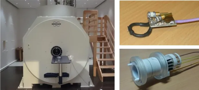
scanners are currently present at NeuroSpin, including three Bruker MRI scanners at 7, 11.7 and 17.2 T dedicated to rodent studies and also two Siemens MRI scanners at 3 and 7 T dedicated to human studies. The 7 T clinical scanner is also equipped with parallel transmission capabilities, allowing to control 8 individual transmission channels for RF coils built for such modality. In this context, the presented work focused on the implementation of 1H and 31P MRS sequences at 17.2 T and their application to study longitudinally normal brain aging in the Dark Agouti rat. In parallel, 1H and 31P MRSI pulse sequences were developed for their application in the human brain at 7 T using multi-channel or single-channel volume coil transceivers.

The presented manuscript is divided in three parts:

The first part explains the methodological context of this thesis. Chapter 1 starts by introducing the fundamental concepts of NMR spectroscopy. Afterwards, it provides a brief presentation of the RF pulses and pulse sequences used as well as related aspects such as energy deposition and chemical shift artifacts. The chapter ends by providing a prospective view of the gains and challenges of MRS at UHF. Chapter 2 presents all the practical considerations and technical implementations. It includes a brief description of the 7 T clinical and 17.2 T preclinical scanners, the implementation and in vitro validation of the BISTRO scheme on both systems as well as the numerical optimization of WET water suppression schemes. The methodology related to the 1H and 31P spectral decompositions using LCModel is presented, detailing the macromolecule baseline parameterization used for the analysis of rat brain 1H spectra. The absolute metabolite quantification strategy for 1H and 31P data is explained. Finally, practical considerations for the acquisition of water T1 maps at 17.2 T are presented.

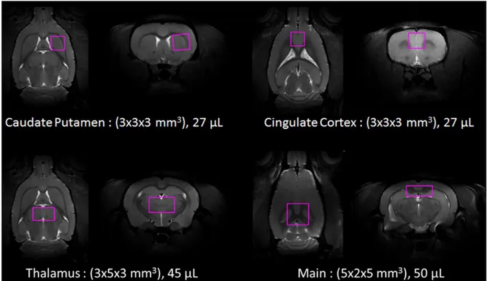
In the second part, the work done at 17.2 T using in vivo quantitative 1H and 31P MR spectroscopy is presented. Chapter 3 presents a longitudinal 1H MRS study of brain aging in the Dark Agouti rat over a span of 18 months. The T1 and T2 relaxation times measured from one

VOI as well as metabolite concentrations from four VOIs in the young rat at 1 month of age are presented. These relaxation times are compared to those measured at lower magnetic fields so as to assess their field-dependency. The evolution of T1 and T2 relaxation times as well as the

neurochemical profiles from the 4 VOIs are then presented and examined using a linear regression analysis. Chapter 4 presents a preliminary 31P quantitative MRS study looking at a subset of our previously studied Dark Agouti rats at ages of 5, 17 and 21 months old. Results from the acquired metabolite profiles and measured T1 times from 8 animals are presented. The

13

The third part presents our MRSI developments and the results obtained on the 7 T scanner. In Chapter 5, the parallel transmission approach is explained along with our methodological framework and the static B1-shim configurations known as the coil eigenmodes or “rings”. The

use of such rings as OVS bands are evaluated and compared to numerically optimized B1-shim

configurations in vitro. Chapter 6 presents the evaluation of 1H and 31P MRI and MRSI sequences for the constitution of a research protocol in the human brain including 1H and 31P metabolite maps acquisitions. The numerically optimized WET scheme is validated in vivo in combination with a 2D CSI-STEAM sequence. Adiabatic and conventional OVS bands configurations are tested and compared in terms of efficiency and energy requirements. The chapter ends showing preliminary in vivo 1H/31P MRSI data.

This thesis ends with a general conclusion summarizing the main results and few perspectives for future work in MR spectroscopy are given.

14

PART

I:

M

ETHODOLOGICAL

C

ONTEXT

1. T

HEORETICAL ASPECTS

1.1. B

NMR

1.1.1. The Zeeman effect

In quantum mechanics, particles such as electrons, protons or neutrons possess an intrinsic angular momentum or spin which may only have discrete values. This angular momentum L depends on the spin quantum number I as:

𝐋 = ℏ √𝐼(𝐼 + 1) ; ℏ = (𝐡 𝟐𝝅⁄ ) (1.1) where h is Planck’s constant and I is integer or half-integer. The spin number I is unique to each nucleus in its stable ground state. For instance, nuclei possessing an odd mass number have a half-integer spin, such as the hydrogen (1H) and phosphorus (31P) which both possess a spin of +1/2. The “direction” or state of the angular momentum is determined by the quantum number m which may have only 2I + 1 values ranging as m = -I, -I+1,…,+I and correspond to the basis states of the particle. The component of the angular momentum in the z direction is given by:

𝐋_𝒛 = ℏ 𝑚. (1.2) The corresponding magnetic moment along the z axis is given by:

µ_𝒛= γ ℏ 𝑚. (1.3) In an external magnetic field B0 oriented along the z axis, the nucleus acquires a magnetic energy

E given by:

E = −µ𝒛 B0 = −γ ℏ 𝑚 B0. (1.4)

This Zeeman effect states that, for a particle with a spin I = 1/2, the energy difference between its two possible quantum states is:

𝚫E = γ ℏ B₀. (1.5) The energy required to transition from one energy state to the other corresponds to a photon or electromagnetic wave with an energy ΔE and a frequency ν0 proportional to the magnetic field B0

15

This resonance frequency is called the Larmor frequency and is given by:

𝜈₀ = (_2𝜋𝛾) B₀ (1.6) The basic principle of NMR is to apply a transverse radiofrequency (RF) wave at the Larmor frequency (usually in the 10 to 103 MHz range) to excite nuclear spins and then detect the electromagnetic wave emitted when the spins return to their lower energy state (figure 1.1B). Notably, equation (1.5) shows that increasing B0 intensity leads to more energy being involved in

the quantum state transitions.

Figure 1.1. The Zeeman Effect and the NMR phenomenon.

A. Upon the application of an external magnetic field B0, quantum energy states for a spin I (= ½) split

depending on its quantum number m (½ or -½). The energy difference between the two spin states is proportional to the magnetic field strength as well as the Larmor frequency of the radiofrequency wave used to excite the spins. B. The number of spins with a preference for the low energy state increases with the magnetic field, leading to higher polarization in the macroscopic sample.

1.1.2. Boltzmann distribution

When considering a macroscopic sample with a large number of spins in an external magnetic field, the methods of Statistical Physics can be used to calculate its macroscopic magnetization. For the case of a population of spins of I = 1/2, only two spin states are allowed: m = +1/2 (µ parallel to B0) or m = -1/2 (µ antiparallel to B0), respectively referred to as the α and β spin states.

Under thermal equilibrium conditions, the two corresponding energy levels are populated according to the Boltzmann probability distribution:

𝑁𝛼

̅̅̅̅, 𝑁̅̅̅̅ =β

exp (±γℏB0⁄2𝑘𝐵𝑇)

exp (−γℏB0⁄2𝑘𝐵𝑇)+exp (γℏB0⁄2𝑘𝐵𝑇) (1.7)

where 𝑘_𝐵 is the Boltzmann equilibrium constant, T is the absolute temperature and 𝑁̅̅̅̅ and 𝑁_𝛼 ̅̅̅̅ β

16

̅̅̅̅ / 𝑁̅̅̅̅ = exp(γℏB𝛽 0⁄𝑘𝐵𝑇) (1.8)

Since at room temperature the thermal energy kBT is five orders of magnitude larger than γℏB0, the population ratio can be approximated to:

𝑁𝛼

̅̅̅̅ / 𝑁̅̅̅̅ ~ 1 +(γℏB𝛽 0⁄𝑘𝐵𝑇) (1.9)

which dictates that for 1H nuclei at 7 Tesla, the population difference between both energy levels or polarization, corresponds to 0.00464 % of the total spin population while at 17 T it increases to 0.0113 %. Due to their lower gyromagnetic ratio and their lesser natural abundance, nuclei other than 1H are more difficult to detect and have lower Larmor frequencies than 1H. Table 1.1 summarizes the NMR characteristics of the nuclei studied in vivo (Bernstein, et al., 2004 p. 960; de Graaf, 2007 p. 9).

Isotope Spin Natural abundance (%) Gyromagnetic ratio γ/2π (MHz/T) NMR frequency in MHz 3.0 T 7.0 T 17.16 T 1 H 1/2 99.985 42.58 127.728 298.03 730.20 2_{H 1 0.015 6.54 19.608 45.75 112.09} 3_{He 1/2 1.4x10}-4 _{32.43 97.302 227.04 556.24} 7_{Li 3/2 92.580 16.55 49.638 115.82 283.76} 13_{C 1/2 1.108 10.70 32.112 74.93 183.57} 14_{N 1 99.630 3.08 9.231 21.54 52.77} 15_{N 1/2 0.370 -4.32 -12.948 -30.21 -74.02} 17_{O 5/2 0.037 5.77 17.316 40.40 98.99} 19 F 1/2 100 40.05 120.156 280.36 686.89 23 Na 3/2 100 11.26 33.786 78.83 193.14 31 P 1/2 100 17.24 51.705 120.65 295.58 39_{K 3/2 93.10 1.99 5.964 13.92 34.10} 129_{Xe 1/2 26.44 11.78 35.331 82.44 201.98}

Table 1.1. NMR properties of most nuclei used for in in vivo NMR studies.

1.1.3. Macroscopic Magnetization

All individual magnetic moments in a sample add up to a net macroscopic magnetic moment M. Although the spins are not parallel to the main magnetic field B0 and have rotational components

on the xy-plane perpendicular to the axis of the static magnetic field (referred as the transverse plane), there is no net transverse component of M as the phase of the spins is randomly distributed. Nevertheless, there will be a net longitudinal magnetization component M0 along the

17

direction of B0 proportional to the population difference N̅̅̅̅̅ − Nα ̅̅̅̅̅ (figure 1.2). From eq. (1.3), β

the expression for M0 at thermal equilibrium can be found:

M₀ = ∑𝑵 µ_𝒊

𝒊=𝟏 = N̅̅̅̅̅µα 𝒛+ N̅̅̅̅̅µβ 𝒛= γ (ℏ₂) (N̅̅̅̅̅ − Nα ̅̅̅̅̅) β (1.10)

where N is the total spin population. At room temperature, one can derive M0 using eq. (1.9):

M0 =Nγ

2_ℏ2

4𝑘𝐵𝑇 B0 (1.11)

This expression reveals the importance of the static magnetic field as well as the gyromagnetic ratio on the magnitude of the macroscopic magnetization. Nevertheless, the interest of the NMR scientist is not the maximum available signal itself but rather the available signal-to-noise ratio (SNR) that is achievable in a given time interval. Other intrinsic factors such as noise levels, sample volume and signal loses due to relaxation time effects also play a role on the determination of the sensitivity.

Figure 1.2. The net magnetization M vector in an external magnetic field.

A. A single spin precesses around the external static magnetic field B0. The spin magnetic moment µ has quantized transverse and longitudinal components. B. The sum of all spin magnetic moments in either the α or β states amount to the macroscopic magnetization vector M. The lack of phase coherence in the transverse plane leaves only a net longitudinal component M0.

1.1.4. Excitation and the Bloch Equations

At the thermal equilibrium state, the net magnetization vector M0 is aligned along the direction of

the main magnetic field B0 and there is no precession motion measurable in the transversal plane.

This precession is needed in order to generate a detectable electromotive force (emf) in an electric circuit through induction (Faraday’s law). Thus, a second transversal magnetic field (B1)

is applied to “excite” the spins and rotate the magnetization towards the transverse plane. In modern impulsional NMR, B1 is applied as a short RF pulse at the Larmor frequency (1.6).

18

frequency, generating an emf in the receiver coil adjacent to the sample.

In practice, an induction coil is used to generate the RF excitation field. For amplitude-modulated RF pulses (discussed in the following section), their duration and intensity will determine the nutation or “flip angle” experienced by the net longitudinal magnetization. Accordingly, the transverse magnetization Mxy reaches its maximum value (Mxy = M0) for a 90° flip angle (figure

1.3).

The evolution of the macroscopic magnetization M under the effects of an external magnetic field Bext composed of both B0 and B1 fields is derived from the following equation:

∂𝐌_∂t = 𝐌 × γ𝐁_𝒆𝒙𝒕 = 𝐌 × γ(𝐁_𝟎+ 𝐁_𝟏) (1.12)

Figure 1.3. Effect of an RF pulse B1 on the macroscopic magnetization M.

At thermal equilibrium, the net magnetization M (= M0) is parallel to the main magnetic field B0. In

order to generate a detectable NMR signal, a time-varying transversal RF pulse B1(t) is applied tilting M about its axis. By calibrating B1 properly, M is rotated by 90° resulting in a maximum amplitude for Mxy. The diagram is shown in the rotating frame of reference at the Larmor frequency.

Taking into account the return to thermal equilibrium, equation (1.12) can be expanded to yield the Bloch equations:

∂M𝑥(t) ∂t = γ[M𝑦(t)B0− M𝑧(t)B1y] − M𝑥(t) T2 (1.13) ∂M𝑦(t) ∂t = γ[M𝑧(t)B1x− M𝑥(t)B0] − M𝑦(t) T2 (1.14) ∂M𝑧(t) ∂t = γ[M𝑥(t)B1y− M𝑦(t)B1x] − M𝑧(t)−M0 T1 (1.15)

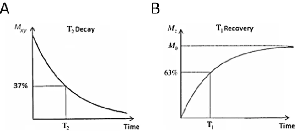
The relaxation times T1 and T2 describe the mono-exponential recovery of Mz and decay of Mxy

19

A. After RF excitation, the transverse magnetization Mxy decreases exponentially with time

corresponding to the dephasing of the spins in the sample. At t = T2, Mxy has been reduced to 37% of

its initial value. B. After RF excitation, the longitudinal magnetization Mz increases exponentially

reaching 63% of its maximal value of M0 at t = T1 and M0 at t>5T1. The T1 relaxation process

corresponds to the spin population’s energy surplus being transferred to its surrounding. In biological tissue, T1 is usually an order of magnitude longer than T2.

1.1.5. Longitudinal relaxation time T

The spin-lattice or T1 relaxation process takes place following a perturbation of the net

magnetization M and determines the speed at which the longitudinal magnetization Mz returns to

its thermal equilibrium value M0. T1 relaxation originates from a constant growth rate of Mz due

to interactions between the excited spins and the lattice, which acts as a reservoir that stocks the energy of the excited spin allowing it to return to its minimal energy state. The relaxation process is done through dissipation of energy into the nearby atoms as thermal energy. The process of energy transfer from the excited spins to the lattice does not induce any increase of temperature in the sample as the proton spin energy is minor compared to the thermal energy scale 𝑘_𝐵𝑇 in

vivo.

From equation (1.15), the time-dependency of Mz can be derived following an excitation pulse: ∂M𝑧(t)

∂t =

M0−M𝑧(t)

T1 (1.16)

Solving this partial differential equation provides the expression of the Mz(t) at time t:

M𝑧(t) = M𝑧(0)𝑒−𝑡/𝑇1+ M0(1 − 𝑒−𝑡/𝑇1) (1.17)

where M𝑧(0) is the longitudinal magnetization just prior to the 90° excitation pulse.

When the experiment is sequentially repeated with a repetition time TR and no residual transverse magnetization remains at the beginning of each repetition, then a steady-state magnetization is achieved after a few repetitions:

20

−TR/𝑇1)

(1−|cos (α)|𝑒−TR/𝑇1) (1.18)

where α is the excitation flip angle (FA). Experimentally, the residual transverse magnetization can be eliminated by applying dephasing gradients or by using a TR longer than 5*T2*. One can

notice that the steady-state magnetization is highest at long repetition times (TR > 5*T1).

However, to optimize the SNR per unit time, one should rather use a short TR (such as TR = T1)

so as to increase the number of signal averages. For a given TR and T1, the optimal excitation

angle or Ernst angle is given by the expression:

α_Ernst = arccos (𝑒−TR/𝑇1) (1.19)

The use of short TRs and corresponding Ernst angle can be an efficient way to accumulate signal in a given time, such as in NMR studies of low sensitivity nuclei like 31P. However, it can be problematic for the quantification of the observed NMR signals especially if they possess distinct T1 relaxation times. Alternatively, long TRs can be used if differential T1-weighting wants to be

avoided, in particular when the T1 relaxation times are unknown.

1.1.6. T

estimation

Several methods are available for the determination of T1 relaxation times:

a) The progressive saturation techniques use the dependency of the steady-state magnetization to the repetition time and flip angle. These methods are suited for low-sensitivity nuclei where long scans are needed to achieve an acceptable SNR or whenever the available scanning time is reduced (Freeman, et al., 1971; Hofmann, et al., 2001; Deoni, et al., 2003; Haacke, et al., 1999 pp. 637-653).

b) The Look-Locker method where several data points with varying T1-weighting are

acquired within a single TR using a single inversion pulse and a train of small FA. This method is time-efficient and allows estimating an apparent T1 relaxation time. Yet it is not

suited for NMR spectroscopy experiments as it requires high SNR (Deichmann, et al., 1992; Schmitt, et al., 2004; Rooney, et al., 2007).

c) The single inversion-recovery (SIR) method consists in acquiring T1-weighted data sets

for which the delay (inversion time = TI) between the inversion pulse and the excitation is varied while keeping a fixed recovery time (= TR - TI) to prevent partial saturation effects (de Graaf, et al., 2006; Vold, et al., 1968; Lu, et al., 2014).

The SIR method (figure 1.5A) is considered the “gold-standard’ for measuring T1 relaxation

times (Cudalbu, et al., 2009; Wright, et al., 2008). After the inversion pulse, the longitudinal magnetization evolves accordingly to eq. (1.17) as:

M_𝑧(t) = −M₀𝑒−𝑡/𝑇1+ M

21

As depicted in figure 1.5B, the return to the thermal equilibrium M0 will depend on the T1 values

of the spin populations in the sample.

In practice, the MRS measurement will consist of numerous repetitions and the steady-state magnetization must be considered instead. For a 90° excitation, the expression is the following:

M𝑧 = M0(1 + 𝑒−TR/𝑇1− 2𝑒−TI/𝑇1) (1.21)

Figure 1.5. Magnetization inversion-recovery method for T1 measurements.

A. Chronogram of the SIR pulse sequence. An inversion pulse is applied at the beginning of the

experiment and an excitation pulse is applied after a delay called the inversion time. The recovery time, corresponding to the delay between the excitation pulse and the next inversion pulse, allows Mz

to reach a steady-state magnetization. B. After inversion of M0,the longitudinal magnetization Mz

recovers at a rate determined by the T1 value. By varying the inversion time, better contrasts can be

observed between spin populations with different T1 times. Measuring Mz at different TIs allows

estimating the T1 value through equation (1.17).

1.1.7. Transverse relaxation times T

and T

The spin-spin or T2 relaxation process takes place in an excited spin population where the net

transverse magnetization decreases in magnitude through dephasing of the individual nuclear magnetic moments. A qualitative explanation of the relaxation process is that spins experience local magnetic fields which are a combination of the main magnetic field B0 and small local

magnetic field changes created by the neighboring molecules. The variation of the local fields leads to fluctuations of the individual precessional frequencies of the spins, which in turn tend to present a different individual phase. This induces a loss in the phase coherence of the excited spin population. The consequence on the macroscopic Mxy component is a reduction in magnitude, the

so-called T2 decay.

From equations (1.13) and (1.14), the time-dependency of Mxy can be derived (for B1 = 0): ∂M𝑥𝑦(t)

∂t = − M𝑥𝑦(t)

22

M_𝑥𝑦(t) = M_𝑥𝑦(0)𝑒(−𝑡/T2) _(1.23)

where M𝑥𝑦(0) is the transverse magnetization just after the excitation pulse.

In practice, there are additional factors to the dephasing of the transverse magnetization, in particular non-random, local magnetic field inhomogeneities ΔB0(r). These local inhomogeneities

are most prominent at the interfaces between media with strong magnetic susceptibility differences, such as brain tissue and air. This apparent relaxation time T₂∗ _{is shorter than the}

intrinsic T₂ relaxation time. Nevertheless, this additional non-random dephasing can be compensated by “refocusing” the individual spins using a spin-echo (SE) or Hahn refocusing pulse sequence (figure 1.6A). If ΔB0(r) is time-independent, the acquired phase of the spins

before refocusing at the position r is:

ϕ(𝑟) = γΔB₀(𝑟) ∗ TE/2 (1.24) where TE/2 is the delay between the excitation and refocusing pulses. As illustrated in figure 1.6B, the application of the 180° refocusing pulse about the xy-plane will cause the individual spins to rotate in the inverse sense prior to the refocusing pulse. Therefore, the phase acquired during the first TE/2 time lapse due the non-random field inhomogeneities will be compensated after the second TE/2 delay. A complete refocalization of the transverse magnetization will occur, forming an echo (figure 1.6B). The TE delay is called the echo-time. The SE sequence is commonly used to estimate T2 relaxation times (figure 1.7).

The measurement of intrinsic T2 relaxation times can be further improved by using a

Carr-Purcell-Meiboom-Gill (CPMG) refocusing pulse train, which is more effective at refocusing diffusion-related dephasing than the Hahn spin-echo sequence. The CPMG pulse train consists of an excitation pulse at time t = 0 and a train of refocusing pulses at time t = (2n+1)τ, where the phase of the 90° RF pulse is shifted by 90° with respect to the n inversion pulses and τ is the middle time-point between the excitation pulse and the first 180° pulse. This phase-cycling approach compensates for imperfections in the refocusing pulse’s flip angles, which otherwise would induce a cumulative error with the number of 180° pulses (Bernstein, et al., 2004 pp. 420-422; Meiboom, et al., 1958).

23

A. The spin-echo pulse sequence consists in a 90° excitation pulse followed by a 180° refocusing

pulse applied at TE/2. The NMR signal is refocused at TE and its intensity is T2-weighted. B. After

excitation, the NMR signal decreases rapidly due to T2 *

relaxation. However, the application of a 180° refocusing pulse leads to the inversion of the spin dephasing in the xy-plane. The phase acquired due to non-random field inhomogeneities before refocusing is cancelled out and a “spin-echo” is formed.

Figure 1.7. Measurement of T2 relaxation times.

After excitation, the transverse magnetization Mxy decays exponentially according to equation (1.23).

By employing a Hahn SE sequence (or better yet, a CPMG refocusing pulse train), T2* effects (and

24

1.1.8. NMR Spectrum and the Discrete Fourier Transform

As it was described in section 1.1.4, when the transverse magnetization Mxy is non-null, a

detectable emf oscillating at the Larmor frequency is induced on the received coil positioned in the transverse plane. Following the T2* decay of the transverse magnetization, a time-varying

complex signal designated as the free induction decay (FID) will be acquired by the NMR spectrometer. This FID can be examined in the frequency domain by applying a complex Fourier transform, resulting in a NMR “spectrum”. In practice, the number of sampled complex values of the FID is finite and the calculation of the spectrum is done instead by applying a discrete Fourier transform (DFT), replacing the theoretical integral by a finite summation. When the number of registered time-points is a power of 2 (such as 2048 = 211) then a fast Fourier transform (FFT) can be applied (figure 1.8) which is computationally more efficient than the DFT (Cooley, et al., 1965; Brigham, 1988).

Once phased, the real and imaginary components of the spectrum correspond to Lorentzian absorption and dispersion lineshapes. For the analysis of the NMR spectrum, the better resolved absorption spectrum is analyzed allowing for the measure of the resonance frequency ν, the peak intensity, area and linewidth at half maximum (FWHM or ν1/2 = ( T2*)-1). If needed, the

spectrum can be analyzed in magnitude but the lineshape is broader due to the dispersive component.

Figure 1.8. Free induction decay and NMR spectrum

The duality between the measured FID in the time domain and its corresponding spectrum in the frequency domain is established by the application of a discrete Fourier transform. The real and imaginary components of the FID and spectrum are shown in blue and red, respectively.

25

1.1.9. Chemical Shift

Nuclei are surrounded by local magnetic fields, in particular the magnetic field created by the movement of electrons in the external magnetic field B0. This induced magnetic field opposes B0

(accordingly to Lenz’s law) and its intensity depends on the density of the electronic cloud around the considered nucleus. Thus, the nuclear spins experience a magnetic “shielding” whose characteristics depend on the molecule the nucleus belongs to or on the molecules in its immediate vicinity. As a consequence, the Larmor frequency will be shifted by a factor σ known as the chemical shift expressed in parts per million (ppm):

ω₀ = 2πν₀ = γ ∗ (B₀− σ) (1.25) A positive σ will correspond to a shielding (higher electronic density) and a negative one will correspond to an anti-shielding (lower electronic density) and it may vary due to changes in the chemical environment such as pH or temperature. The definition of the chemical shift of a group of equivalent nuclei is:

σ=𝜈0−𝜈𝑟𝑒𝑓

𝜈𝑟𝑒𝑓 (1.26)

where 𝜈_𝑟𝑒𝑓 is the resonance frequency of a reference compound. The standard reference compounds used for system and coil calibrations is tetra-methyl-silane (TMS) for 1H MRS and phenyl-phosphonic acid (PPA) or hexa-methyl-phosphorous-triamide (HMPT) for 31P MRS.

1.1.10.

J-Coupling

When two nuclei are involved in a covalent bound, the nuclear spins interact indirectly through their shared electrons. This scalar, spin-spin or J- coupling results in a splitting of their respective resonances into hyperfine structures. Scalar coupling originates from intramolecular coupling mechanisms, in contrast with dipole-dipole interactions which take place between different molecules.

In it most simple case, two bounded atoms A and X with a large gap in resonance frequencies are considered (figure 1.9A). By the Pauli Exclusion Principle, the interaction between the electrons inside the covalent bond is forced to be antiparallel. In the case where the AX spin system is in the high-energy (ββ) or low energy states (αα), one of the nuclei (say A) will be in a parallel spin state to that of its electron, which is less favorable than an antiparallel state. The energy level will therefore increase by an amount of JAX/4 where JAX corresponds to the single-bond scalar

coupling constant between A and X. For the intermediate states (αβ and βα), the electrons can be in antiparallel state with the nuclei spins which is energetically favorable, decreasing the energy levels of these states by JAX/4. In the case of heteronuclear coupling such as A = 1H and X = 13C,

26

spectrum consists in a pair of resonances centered on the Larmor frequency with a JHC frequency

gap (figure 1.9B). In the case of a strongly coupled system AB in which the difference in resonance frequencies is small (|𝑣_𝐴 − 𝑣_𝐵| ≈ JAB), there are still 4 energy level transitions but the

intensities of the corresponding NMR resonances are distorted by second order effects. Notably, J-coupling constants are independent of the magnetic field intensity.

Figure 1.9.Energy levels splitting due to J-coupling and NMR spectrum of a weakly-coupled AX spin system. A. Two atoms interacting through a covalent bond are linked through an electron bond. The energy levels of the spins A and X are influenced by the anti-parallel pairing of the electrons due to the Pauli Exclusion Principle. This scalar coupling JAX leads to 4 different possible energy states. B. This

leads to 4 possible single spin transitions (E2-E1 and E4-E3 for A and E3-E1 and E4-E2 for X). If it is a

weakly-coupled spin system (|𝑣_A− 𝑣_X| ≫ J_AX), the NMR spectrum consists in 2 doublets of resonances centered on the Larmor frequencies of A and X each with a JHC frequency gap.

27

1.2. MRS

S

1.2.1. Radiofrequency Pulses

1.2.1.1. Amplitude Modulated Pulses

As explained in section 1.1.5, the longitudinal magnetization is projected towards the transverse plane by applying a secondary transverse magnetic field B1 oscillating at or close to the Larmor

frequency of the spin population of interest. The B1 “excitation” field is created by a surface or

volume transmit coil. The resolution of the Bloch equations (eq 1.13-1.15) during the application of the RF “pulse” B1(t) allows for the calculation of the magnetization M(t). To do so, it is

convenient to describe the NMR experiment in a frame rotating about B0 at the angular carrier

frequency  as well as an effective magnetic field Beff:

B_eff = √B₁2_{+ (}Δω γ )

2

; Δω= ω₀ − ω (1.27) with 0 being the angular Larmor frequency.

On-resonance (B1 ≫ Δω

γ ), the magnetization rotates about B1 as shown in figure 1.3 and the FA α

is given by:

α= γB₁𝑇 (1.28) with T being the RF pulse duration. However, off-resonance effects are present when the frequency offset Δ is comparable to γB1. In MRS, this is usually the case since the spectral

bandwidth is several kHz wide.

By incorporating Beff into the Bloch equations, frequency-dependent profiles of the three

magnetization components Mx, My and Mz can be calculated. A simpler method to estimate the

frequency profile of the RF pulse is to apply a Fourier transformation (FT) in the time domain. Yet, the FT being a linear operation, it must be taken into consideration that the said frequency profile is an approximation only valid for small nutation angles (α<30°) where the sinus function is almost linear (sin(α) ≈ α).

Another important factor for the characterization of RF pulses is the Time-Bandwidth or R factor. The R factor corresponds to the product of the pulse length T and the pulse bandwidth Δ. The latest is measured as the full width at half maximum (FWHM) of the frequency profile of the resulting magnetization after a 90° or 180° FA for excitation and inversion/refocusing pulses, respectively. For a given RF pulse modulation, the R factor is constant and is useful for determining the pulse duration needed to achieve a target bandwidth:

28

normalized square pulse of the same duration: κ= √(∑ 𝑉𝑵 _{𝑖,𝑅𝑒𝑎𝑙} 𝒊 ) 𝟐 + (∑ 𝑉𝑵 _{𝑖,𝐼𝑚𝑎𝑔} 𝒊 ) 𝟐 𝑵 ⁄ (1.30) where V is the (discrete) vector representation of the pulse envelope defined by N complex points. The amplitude integral κ is useful for calculating the required B1 for a particular pulse and

a desired flip angle, provided that a reference value is available from a reference pulse (usually a 1 ms long square pulse). The mathematical expression is directly derived from eq. (1.28):

α= γ ∗ B₁∗ 𝑇 ∗ κ (1.31) The choice of a RF pulse will largely depend on the experimental demands and constrains, such as spectral bandwidth and desired sharpness (transition bandwidth), available RF power, gradient capabilities and Specific Absorption Rate (SAR) limitations. The R and κ factors for the most common AM pulses used during this thesis are listed in table 1.2.

The transition bandwidth Tbw is the frequency gap for which the condition 0.05 ≤ Mxy/M0 ≤ 0.95

holds for a 90° excitation pulse and it should be considered when sharp excitation profiles are required. Sinc pulses with a high number of lobes have good Tbw while Gaussian pulses have

rather degraded ones but demand a smaller B1max. Hermitian shaped pulses show a good

compromise between Tbw, R value and peak B1.

Pulse Shape Time-Bandwidth R Amplitude Integral κ

Gaussian 2.17 0.5530

Sinc 3-lobes (FLASH,Siemens) 3.35 0.3504

Sinc 3-lobes (CSI,Siemens) 3.84 0.2800

Sinc 7-lobes 8.92 0.1137

SLR (VERSE)a 15.00 0.1049

Square 1.37 1.0000

Hermitian 5.43 0.1794

Table 1.2. Time-Bandwidth product and amplitude integrals of common AM pulses.

a

(Amadon, et al., 2010)

1.2.1.2. Adiabatic Pulses

In most MRS studies, surface coils are used due to their high sensitivity and elevated peak power. Nevertheless, they generate a quite inhomogeneous B1 excitation field, leading to artifacts when a

29

the plane of the transmitter’s inductive loop(s). Although it is possible to solve the B1

inhomogeneity problem by using a transmit-only volume coil in conjunction with a receive-only surface coil, the maximum B1 power needed to apply high-bandwidth RF pulses can be

compromised (aside from the increasingly complicated set-up and possible coupling effects). An elegant and reliable solution consists in using RF pulses for which the FA will be less sensitive to the amplitude of the applied B1. Adiabatic pulses are frequency- and amplitude-modulated pulses

that generate a uniform nutation angle even in an inhomogeneous B1 field provided that the RF

amplitude is above a certain threshold so that it stays in the adiabatic regime.

A qualitative illustration of the application of an adiabatic pulse is as follows. The frequency modulation on the applied B1 field has an effect equivalent to modulating the off-resonance

component of Beff as shown in equation (1.27), where  is substituted by the term Δω(t) =

ω(t)-ω0:

B_eff(t) = √B₁2(t) + (Δω(t)

γ ) 2

(1.32) Through the simultaneous modulation of the RF field intensity and carrier frequency, the effective Beff(t) field changes in orientation over time. If the orientation (with respect to the

reference frame rotating at the Larmor frequency) given by: α(t) = arctan (_γBΔω(t)

1(t)) (1.33)

changes slowly enough such that it complies with the adiabatic condition:

|dα(t)_γdt | ≪ |Beff(t)| (1.34)

then the magnetization that was parallel (Mz) and perpendicular (Mxy) to Beff at the beginning of

the RF pulse will keep their orientation to Beff(t) for the duration of the pulse. If this condition is

not fulfilled, there will be a loss of coherence among the longitudinal magnetization vectors at different frequencies according to Δω(t) and B1.

Adiabatic pulses can be easily calibrated by keeping a constant pulse length and gradually increasing the transmitter power up to a threshold at which the recorded signal intensity remains constant. The most commonly used adiabatic pulses are the hyperbolic secant (HS) adiabatic half-passage (AHP) 90° excitation pulse and the adiabatic full-passage (AFP) 180° inversion pulse (Silver, et al., 1984; Baum, et al., 1985), whose amplitude and frequency modulation functions F₁(t) and F2(t) are:

B1(t) = B1 max∗ F1(t) = B1 max∗ sech [βτ(t)] (1.35)

Δω(t) = ωc+ Δωmax∗ F2(t) = ωc+ Δωmax∗tanh [βτ(t)]_{tanh [β]} (1.36)

where τ = (1-2t/Tp), Tp is the pulse length, β is a truncation factor close to 5.3 so that sech(β) =

30

effective excitation bandwidth is B1 dependent as the angle α(t) for off-resonance excitation

varies with Δω and B₁ as shown by eq. (1.40). It is worth noticing that AHP and AFP pulses are not plane rotations as the existing transverse magnetization Mxy at the start of the pulse rotates

around the effective field Beff acquiring a linear phase as a function of the RF intensity and the

frequency offset, effectively dephasing during the pulse. However, if an AFP pulse has been applied, running a second AFP just afterwards inverts the effective field Beff canceling the

acquired linear phase by adding the same opposite phase to the magnetization vector. This method of adiabatic refocusing is employed by the LASER localization sequence as it will be discussed later on this chapter.

When the power requirements are too elevated for the spectrometer or the SAR levels are too high, other modulation functions can be used to reduce the maximum required RF amplitude B1max while degrading moderately the transition bandwidth of the pulse profile. Modulating

function pairs F1 and F2 may be used as long as they fulfill the Offset-Independent Adiabaticity

(OIA) condition:

(γB1 maxF1(tΩ))

2

Δω_maxF2(tΩ)

≫

at time tΩ for an on-resonance frequency isochromat Ω. As it was shown by Tannus and

Garwood (Tannùs, et al., 1997), the peak power of OIA pulses is determined by the AM function while the average power is determined by the inversion bandwidth (for a fixed pulse duration TP).

Among the modulating functions that fulfill the OIA conditions, the HSn pulse family was used in this thesis to limit the required B1max. Their AM and FM functions are given by the formulas:

F1(t) = sech (βτ𝑛(t)) (1.38)

F₂(t) = ∫ sech 2_(βτ𝑛_{(t)) (1.39)}

The use of HS8 (n = 8) pulses with respect to the standard HS AFP shows a dramatic improvement in the required peak power, as there is a 51% reduction in B1 max while the average

applied power changes by less than 1% (TP = 2ms, Bandwidth (Ω) = 50 kHz). Nevertheless, Tbw

is degraded by 5%.

1.2.1.3. Energy deposition

Along with the magnetic field B1, an associated electrical field E is created which induces

electrical currents in the sample. These induced electrical currents are dissipated into heat which may become harmful if the ensuing increase in temperature reaches a hazardous level, particularly in tissues with low perfusion. The local temperature elevation at a position r depends on the conductivity σ(r) and density ρ(r) of the tissue as well as the duration T of the local

31

electric field E(r,t). The level of energy deposition is determined through the specific absorption rate (SAR) and is given in watts per kilogram.

The IEC has determined safety guidelines (International Electrotechnical Commission, March 2010) based on global and local SAR limits over periods of integration of 6 minutes and of 10 seconds. Global SAR corresponds to the energy deposition on the entire head and local SAR on the energy deposition over the mass of any closed 10-grams volume. The local SAR is limited to a maximum of 20 W/kg over a period of 10 seconds and 10 W/kg over a 6-min window. The global SAR is limited to a maximum of 9.6 W/kg over a period of 10 seconds and 3.2 W/kg over a 6-min window. The local SAR can be calculated using the following expression:

𝑆𝐴𝑅𝑙𝑜𝑐𝑎𝑙(𝑟) = _2𝜌(𝑟)𝜎(𝑟) _𝑇1∫ ‖E(𝑟, t)‖₀𝑇 2𝑑𝑡 (1.40)

The E-field depends on the transmitter coil and quality factor as well as the characteristics and positioning of the sample within the coil. Global energy deposition can be calculated based on the quality factor of the loaded and unloaded coil, but this information does not provide information about the eventuality of local “hot-spots” (Haacke, et al., 1999 pp. 858-860). From the SAR mathematical expression, it can be observed that:

1) the power deposition scales quadratically with the intensity of the electric field,

2) for a given flip angle, SAR values can be reduced by increasing the duration of the pulse (at the cost of decreasing its spectral bandwidth) and

3) longer TRs may help overcome SAR limitations at the cost of longer acquisition times.

1.2.2. SVS localization

Spatial localization of the NMR signal is an essential aspect of in vivo MRS. In order to acquire physiologically relevant and good quality spectra, a proper localization sequence must be used to select the NMR signal from within the VOI and avoid spurious signal from outside. Indeed, localization errors introduces unwanted signal that biases the validity of a spectrum for physiological or clinical research purposes. Furthermore, experimental adjustments such as the B0

and B1 field homogenization or “shimming” and RF pulses calibration are spatially-dependent.

Therefore, a good spatial localization will guarantee that the NMR signal is originating from a region where experimental conditions have been optimized hence improving the quality of the spectra. It will also confine the NMR experiment to the VOI and minimize partial volume effects. Using high-bandwidth RF pulses for spatial selection is an efficient way to limit the mismatch between the volumes localized for spins resonating at different frequencies. This artifact is detailed in section 1.2.4 and is known as the chemical shift displacement artifact (CSDA).

Single volume spectroscopy (SVS) sequences that were most relevant to this work are briefly described below.