Inertial regimes in a curved electromagnetically forced flow

HAL Id: hal-01419450

https://hal-ensta-paris.archives-ouvertes.fr//hal-01419450

Preprint submitted on 19 Dec 2016

HAL is a multi-disciplinary open access

archive for the deposit and dissemination of

sci-entific research documents, whether they are

pub-lished or not. The documents may come from

teaching and research institutions in France or

abroad, or from public or private research centers.

L’archive ouverte pluridisciplinaire HAL, est

destinée au dépôt et à la diffusion de documents

scientifiques de niveau recherche, publiés ou non,

émanant des établissements d’enseignement et de

recherche français ou étrangers, des laboratoires

publics ou privés.

Inertial regimes in a curved electromagnetically forced

flow

Jean Boisson, Romain Monchaux, Sébastien Aumaître

To cite this version:

Jean Boisson, Romain Monchaux, Sébastien Aumaître. Inertial regimes in a curved electromagnetically

forced flow. 2016. �hal-01419450�

Inertial regimes in a curved

electromagnetically forced flow

J. Boisson

†, R. Monchaux

and S. Aumaˆ

ıtre

1

IMSIA, ENSTA ParisTech, CNRS, CEA, EDF, Universit´e Paris-Saclay, 828 Boulevard des Mar´echaux, 91762 Palaiseau Cedex France

2

SPHYNX, Service de Physique de l’Etat Condens´e, CNRS UMR 3680, CEA Saclay, F-91191 Gif-sur-Yvette Cedex, France

3

Laboratoire de Physique de l’ ´Ecole Normale Sup´erieure de Lyon, CNRS and Universit´e de Lyon, 46 all´ee dItalie, F-69364 Lyon cedex 07, France

(Received 16 December 2016)

We investigated experimentally the flow driven by a Lorentz force induced by an axial magnetic field −→B and a radial electric current I applied between two fixed concentric copper cylinders. The gap geometry corresponds to a rectangular section with an aspect ratio of η = 4 and we probe the azimuthal and axial velocity profiles of the flow along the vertical axis by using ultrasonic Doppler velocimetry. We have performed several runs at moderate magnetic field strengths, corresponding to moderate Hartmann numbers M 6 300. At these forcing parametersand because of the geometry of our experimental device, we show that the inertial terms are not negligible. This induces the azimuthal velocity that depends on both I and B.From measurements of the vertical velocity we focus on the characteristics of the secondary flow: the time averaged velocity profiles are compatible with a secondary flow presenting two pairs of stable vortices as pointed out by previous numerical studies. We exhibited a transition between two dynamical modes, a high and a low frequency one. The high frequency mode, which emerges at low magnetic field forcing, corresponds to the propagation in the r-direction of tilted vortices. This mode is consistent with our previous experiments and with the instability described in Zhao et al. (2011) taking place in an elongated duct geometry. The low frequency mode, observed for high magnetic field forcing, consists in large excursions of the vortices. The dynamics of these modes matches the first axisymmetric instability described in Zhao & Zikanov (2012) taking place in an square duct geometry. We demonstrated that this transition is controlled by the inertial magnetic thickness H′ _{which is the characteristic}

length we introduce as a balance between the advection and the Lorentz force. The key point here is that when the inertial magnetic thickness H′_{is comparable to one geometric}

characteristic length (H/2 in the vertical or △r in the radial direction) the corresponding mode is favored. Therefore, when H′_{/(H/2) ≈ 1 we observe the high frequency mode}

taking place in elongated duct geometry, and when H′_{/△r ≈ 1 we observe the low}

frequency mode taking place in square duct geometry and high magnetic field.

Key words:moderate-Hartmann-number flows, magnetohydrodynamics, secondary flows, regimes transition

1. Introduction

In Magnetohydrodynamic flows (MHD) the retroaction of the fluid on the magnetic field is controlled by the magnetic Reynolds number Rm (Moffatt (1978)). At the low-Rm regimes considered here, the induction is negligible. An external electric current density,−→j , is applied to ensure the presence of a significant Lorentz force−→j ×−→B , where −

→_{B is the magnetic field. This forcing imposes the configuration and the properties of} the flow. Although it is intrinsically a volumic force, in extreme regimes with a high enough magnetic field, the diffusion of momentum by the Lorentz force suppresses the velocity gradient over a large diffusion length. In this region no current can exist, then the imposed electric currents are constrained in flow boundary layers, letting the fluid bulk Lorentz-force free and quasi two dimensional (Moreau (1990)).

The thickness of these so-called Hartmann layers (eH), defined by the balance between

the viscous term and the Lorentz force in the Navier Stockes equation, is controlled by the inverse of the Hartmann number M , which only depends on the magnetic field and on some properties of the liquid : M = HBpσE/(ρν)/2 with H the characteristic length

along the magnetic field direction, σE the electric conductivity, ρ the volumic mass and

ν the kinematic viscosity of the fluid. By the channeling of the currents near the top and bottom plate into the Hartmann layer, the magnetic field also generates a boundary layer near the axial electrode, called the Shercliff layer, which is assumed to scale like 1/√M (Hunt & Stewartson (1965)).

As mentioned above, one of the main action of the magnetic field is to reduce the velocitygradientsin its direction and hence to yield the flow two dimensional (Sommeria & Moreau (1982); Poth´erat (2012)). In this context, several authors studied experimen-tally and theoretically the flow produced in a Taylor-Couette like geometry with steady cylinders where only the Lorentz force drives the flow. Baylis & Hunt (1971) showed that the azimuthal velocity only depends linearly on the electric current forcing under the assumption of negligible inertial effects and in the large Hartmann number limit. The profile of the azimuthal velocity vθ was computed in an infinite cylinder neglecting the

induction effects by Digilov (2007) and Zhao et al. (2011). Such a velocity profile close to a Poiseuille profile at low Hartmann number becomes unstable according to the Rayleigh criterion for M >> 1 (Chandrasekhar (2013)). Tabeling & Chabrerie (1981) studied sec-ondary flows at high Hartmann numbers in the early 1980’s. They demonstrated that its configuration depends on the conductivities of the walls and they introduced a more stringent criterion for inertial effects to be negligible. Later, Tabeling (1982) reported experimental evidences of instabilities for a limited range of forcing in a device with η = H/(ro− ri) = H/△r ≫ 1 with H the cell height, ro and ri the outer and inner

radius respectively. The same geometry with a square section (η = 1) has been used to study the laminar-turbulence transition by Moresco & Alboussiere (2004). They showed that the control parameter of the transition is a Reynolds number based on the Hartmann layer thickness as Re/M (Re = U0△r/ν with U0 the mean azimuthal velocity). This is

due to the fact that the thickness of the Hartmann layer will prevent the transition to turbulence even at large Reynolds number. Several numerical studies of this particular geometry have been performed. Krasnov et al. (2004) attributed the discrepancy in the instability threshold values found between the experimental data and the linear stabil-ity analysis to finite-amplitude perturbations. Vantieghem & Knaepen (2011) (at low Reynolds number) and Zhao & Zikanov (2012) (at high Reynolds and Hartmann num-bers) show the presence of two pairs of contra-rotating vortices. One is arranged along the inner axial wall while the other is arranged along the outer axial wall. However, to our knowledge, the configurations of the secondary flow before the establishment of the

fully developed Hartmann regime (M >> 1) were not studied experimentally. This is the purpose of the present article that presents runs at moderate Hartmann number in a domain where the inertial effects cannot be negligible.

Due to the difficulty in using usual anemometry techniques in liquid metals as described in Shercliff (1965), velocity has never been directly measured in the previous experimen-tal studies. Local or global potential measurements were performed instead. However, measurements of velocity profiles using ultrasonic techniques can actually be achieved in liquid metal flows as first demonstrated by Brito et al. (2001) and Eckert & Gerbeth (2002). Since then, several experimental studies have used this technique: Boisson & Au-maitre (2012) to characterise travelling waves in a MHD flow and more recently Stelzer et al.(2015a) and Stelzer et al. (2015b) to study the base flow and its instability in an electrically driven magnetohydrodynamic flow with a free Shercliff layer.

This manuscript presents a series of behaviors that trace back transitions between dif-ferent dynamical regimes controlledby the characteristic length of velocity gradients H′

and the corresponding Reynolds number R′ _{(that will be precisely defined in section 3).}

Its layout is the following. After a short description of the experimental device in section 2,we evaluate, in section 3, the importance of inertial effects in our flow. Based on this, we determine a scaling U0 for the azimuthal velocity in our system depending on the

ap-plied electrical current and magnetic field.We show the key role of the inertial magnetic thickness we introduced as the balance between the non-linear advection and the Lorentz force. This scalingrelies on a force-free region different from the classical one associated to Hartmann layers but similar to even if different from the one in Duran-Matute et al. (2011) and Poth´erat & Klein (2014). It agrees with our measurements and is used to define the key non-dimensional numbers of our system. In section 4, we determine the time average of axial velocity profiles and we identify the transition to the growth of the inertial magnetic thickness beyond the size of the apparatus gap. In section 5, we focus on the two dynamical regimes that we characterize. They are compared to former numerical studies by Zhao et al. (2011) and Zhao & Zikanov (2012) in section 6. Conclusions are drawn in the last section.

2. Experimental setup

The experimental device, which takes over the one described in Boisson & Aumaitre (2012) with a larger aspect ratio, is sketched in figure 1. In a Taylor-Couette like geometry, an azimuthal Lorentz force is generated by a radial current I and an axial magnetic field −→B in order to force a cylindrical layer of liquid metallic alloy: the Galinstan. The Galinstan is made of 68.5 % of Gallium, 21.5 % of indium, 10 % of Tin. Its density is ρ = 6.440 × 103

kg/m3

, its kinematic viscosity is ν = 3.73 × 10−6 _m2

/s, its electrical conductivity σ = 3.46 × 106

(S/m). In the design of the experiment, a special care has been devoted to the homogeneity of the input current and magnetic field, without fluid motion. To this aim, the inner and the outer cylinders used as electrodes are made of a large mass of copper. This is also why we divide the current departures in eight axisymmetric locations on the lateral surface for the outer cylinder and the current arrivals in two locations on the top and bottom of the inner cylinder. The resistivity of the overall device is less than 0.1 Ohm and is mainly due to wiring and connectors. The plastic covers induce insulating boundary conditions where the Hartmann layers develop. The annular duct height is H = 120 mm, its width is △r = 30 mm, the inner and outer radius are ri = 10 mm and ro= 40 mm respectively. This imposes the mean

radius r = 25 mm. The resulting aspect ratio is η = H/△r = 4. Radial inhomogeneity of the applied magnetic field is less than 3% within the fluid gap with an axial variation

1 2 3 B △r I I H US Probe − →_v θ ri ro − →_e r − →_e z Hartmann layer

Figure 1.Axial cut of the experimental device. The liquid alloy (in yellow-green) is enclosed between two coaxial copper cylinders (in coppery color shading) of radius ri= 10 mm and ro

respectively with △r = ro− ri= 30 mm. The cylinder height is H = 120 mm and the aspect

ratio is η = H/△r = 4. The inner and outer cylinders, used as electrodes, are made of large masses of copper. A homogeneous current is provided by two inputs on the top and bottom of the inner cylinder and eight symmetrical departures on the outer cylinder. The top and bottom covers are electrically insolating. The three locations of the ultrasonic probes are situated on the bottom of the channel gray shading enumerated 1, 2, 3

never exceeding 4.5% and symmetric with respect to the mid-plane of the cell. The coil can produce magnetic fields up to 0.15 T, while the radial current crossing the cell can be controlled up to 100 A. vθ and vz are respectively the azimuthal and axial velocity

components. The spatial and temporal averages will be noted h·i and · respectively. We used an ultrasonic Doppler velocimeter DOP3010 from Signal processing with two probes which extract the projected velocity along their axis from phase correlation of two ultrasound pulses (USP). The USP are scattered by Galinstan oxides present in the media. The probes can be placed at different locations with slightly different angles, three locations at r1 = 16, r2 = 25 and r3 = 34 mm with an angle of 0◦ and one at

r2 = 25 mm with an angle of 5◦ with respect to the cylinder axis (z). As vθ is deduced

from a geometric reconstruction based on the two US probes at different angles as detailed in Boisson & Aumaitre (2012), we only have access to its time average vθ(z). Each profile

is estimated from a sampling of 500 points along the z axis. This corresponds to a spatial resolution ∆z = 0.2 mm. We recorded at least 500 profiles per probe per measurement. The emitting frequency of the ultrasounds is 4 MHz. The temporal resolution, defined by the time delay between successive pulses, ranges from ∆t ≈ 0.2 s to ∆t ≈ 0.04 s for faster regimes. This value depends on the maximum velocity of the flow, the sound speed in the material, and the numbers of sound pulses needed to reconstruct the velocity profile. Multi-reflections of the ultrasound beam on the Galinstan-polycarbonate interface add systematic noise to the first 15 mm of each velocity profile. It is worth noticing that the

volume explored by the ultrasound beam is not constant along its emitting axis. There is a tightening of the beam up to the near field limit at about 30 mm from the probe extremity, then the beam diverges with a diffraction angle of 2◦_{. This implies that the}

velocity values measured are actually integrated over a sampling volume centered on the beam axis. The width of this volume is about 3 mm at the mid-height of the cell. Two kinds of runs were realized. The first one, named type I hereafter, is dedicated to the determination of the mean configuration of the secondary flow. The procedure is the following.We wait for the permanent regime to be established before recording 500 profiles per probes, one probe after another. The length of the transient regime is appreciated using the direct visualization of the velocity profiles captured by the probes. The second kind of runs, named type II, is dedicated to the dynamical behavior. Here, we also waitfor the permanent regime to be establishedand then we record alternatively a profile on each probe. The procedure is repeated at least 500 times and up to 2000 times at a rate of about 10 profiles per second in order to access the flow dynamics. Runs were performed at five different Hartmann numbers (M = 45, 114, 182, 250, 318), corresponding to a magnetic field−→B ranging from 0.02 to 0.14 T, to an electric current I ranging from 1 A to 100 Aand to Reynolds numbers ranging from 12000 to 42000. It has to be noted that, as we only have two probes, 2 different runs at the same forcing had to be performed to get the mean profile at the three radial locations. The probe at r2= 25 mm is always operating and is used to validate the measurement reproducibility

by comparing the mean profiles acquired by this probe during 2 similar runs.

3. Dimensionless numbers and scaling of the azimuthal velocity

Usually, for high magnetic field M ≫ 1, in the case where the inertial terms are negligible, the thickness in which electric currentsare concentratedis deduced from the balance between the Lorentz force and the viscous drag. Thus, in this case it reduces to the Hartmann layer eH = 1/(pσ/(ρν) · B).Neglecting Hartmann friction with respect

to inertial effect is possible when its characteristic time scale becomes large with respect to the inertial one. Their ratio goes as Re/M which is always larger than 30 in our high curvature geometry and for our range of Reynolds numbers. Thus, the main contribution balancing the Lorentz force in the Navier-Stokes equations is the advection term.In order to test that assumption, we adapted the dimensionless number introduced by Baylis & Hunt (1971) to a rectangular section. With our definition of the Reynolds and Hartmann numbers, the inertial term is predominant if:

Re2 M4 × H4 16△r2_r2 ≫ 1, (3.1) Ba = H 4

16_△r2r2 is a dimensionless coefficient taking into account the geometry to ponder the interaction parameter N = _ReM42.The influence of this coefficient can be important: for example, in the present work Ba ≈ 23 and in the Zucchini device used by Stelzer et al.

(2015a) Ba ≈ 1.5 × 10−2, explaining why both experiments explore completely different

regimes even if both present comparable interaction parameters.

In figure 2 we compare the explored ranges of BaN−2 in several studies using similar

geometries than the one we present here. This figure illustrates that our investigation of flows where inertial effects can be predominant are done for the first time to our knowledge with direct ultrasound measurements. Indeed, Baylis (1964) only focused on demonstrating the feasibility of using electric potential measurements to show insta-bilities in liquid metal flows. Later, Baylis (1971) pointed out, with electric potential

10

10

10

10

10

10

10

Baylis (1964) Baylis (1971) Tabeling (1982)

Moresco & Alboussiere (2004) Mikhailovich et al. (2012) Zhao et al. (2011)

Zhao & Zikanov (2012) Stelzer et al. (2015a)

Boisson & Aumaitre (2012) Present work

Khalzov et al. (2010)

BaN−2

Figure 2.Comparison of the explored values of the dimensionless number defined in Baylis & Hunt (1971) which compares the inertial term to viscous term for different works. The reported studies are classified chronologically along the vertical axis. The blues ones are experiments were the velocity measurements system is based on the electric potential. The red ones are numerical studies. The yellow/orange ones are experiments were the velocity measurements system is based on ultrasound.

measurements, changes of the friction factor dependance that could be related to the transition between the inertial regimes to the viscous regimes, as his range of parameter BaN−2 spans on both parts. Tabeling (1982), Moresco & Alboussiere (2004) and Stelzer

et al. (2015a) focused on regimes where the viscous balance holds, while Mikhailovich et al.(2012) investigated the decay of mean velocity components and turbulent fluctu-ations. The numerical works of Zhao et al. (2011) and Zhao & Zikanov (2012), that we compare our results with, cover both regimes. The latest work can be compared to ours only in the more extreme regimes we explored, that is to say when BaN−2 < 1.

Therefore, if we balance the Lorentz force by the inertial term in Navier-Stokes equa-tion, it follows: U2 0 H′ ∼ JB (ρ), (3.2)

where U0 is the mean azimuthal velocity scaling and H′ is the characteristic length

of the velocity gradient. In the following, we will refer to H′ _{as the inertial magnetic}

thickness. We define the bulk as the region where the total current vanishes, letting the flow supposedly force-free. Consequently, the characteristic length of the velocity gradient corresponds to the layer thickness where the electric currents are constrained. From these assumption and definition, we determine that radial current density J in this layer corresponds to the total applied current over the section of fluid:

0

0.1

0.2

0.3

0.4

0

0.2

0.4

0.6

0.8

1

1.2

1.4

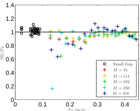
Figure 3.The ratio of the experimental mean azimuthal velocity value over the scaling hvθi/U0

as a function of U0. The circles corresponds to values extracted from the small gap device from

Boisson & Aumaitre (2012) (corresponding to △r = 12 mm and ˜r = 93.3 mm), the crosses correspond to the values measured in the larger gap presented here (corresponding to △r = 30 mm and ˜r = 13 mm). Colors encode the five tested Hartmann numbers according to the legend.

J ∼ _rH˜I_′, (3.3)

with ˜r = riro

△r a dimensional parameter taking into account the variation of the current

density imposed by the device geometry and H′ _{the thickness of the layeralong zwhere}

the current is present. This only holds if H′ _{is smaller than H/2. This definition}

re-minds the Lorentz force diffusion length introduced by Duran-Matute et al. (2011) and Poth´erat & Klein (2014), the difference being that we consider here the total Lorentz force (including the gradient part due the radial currents).

Then, by replacing 3.3 into 3.2 H′ _{cancels and the azimuthal velocity scales like :}

U0∼

s IB

(˜rρ). (3.4)

Note that this scaling still holds for H′ _{> H/2. In that case H just replaces H}′ _{in 3.3}

and 3.2.

From our definition of the bulk as the force-free region, using the fact that the bulk velocity is mainly in the azimuthal direction, we can infer that the induced radial current density is:

Combining equations 3.4 and 3.5 we obtain : H′∼ _σB13_/2

r ρI ˜

r . (3.6)

This latter scaling is obviously valid only if H′ _{6 H/2. In our experimental setup we}

observe that H′ _{is large compared to the Hartmann layer thickness (H}′ _{> 40e} H) but

it is rather comparable to the gap width (0.25 6 H′_{/△r 6 25) and to the cell height}

(0.06 6 H′_{/H < 4.2).We thus expect important effects to be observed when H}′ _gets

comparable to the system height, H.

We experimentally test these scaling laws. First we determine the mean azimuthal veloc-ity value hvθi by reconstructing the azimuthal velocity profile from the mean profiles

mea-sured at r2 with two different angles. Then we average this profile between z1= 30 mm

and z2 = 90 mm to focus on velocity values in the bulk. In figure 3, we compare the

experimental azimuthal velocity extracted from the large gap device of figure 1 (colored crosses) and from the one reported in Boisson & Aumaitre (2012) (black circles) to:

U0≈ 2.1

s IB

(˜rρ)− 0.015. (3.7)

Regardless of the aspect ratios, the agreement is very good with only two adjusted nu-merical parameters. It thus justifiesthe scaling proposed in equation 3.4. The prefactor probably only depends on the experimental device specifications (ohmic resistance of the electric cables, cylinders composition and thickness, . . . ) and the offset takes into account the viscous linear behavior at low forcing. It has to be noted that U0 depends both on I

and B in contrast with the work of Baylis (1971) or Stelzer et al. (2015a) for example. Because most of our runs are performed at BaN−2>1, inertial effects still holds, thus,

in our case, the electric currents are not constraint to Hartmann layers. Then the rele-vant non-dimensional parameters are the Reynolds numbers which ranges from 12000 to 42000 and R′ _{which is the Reynolds number based on the inertial magnetic thickness H}′_:

R′≡ H

′_U0

ν ≡ I

σν ˜rB. (3.8)

We must stress that R′ _{and H}′ _{are both increasing functions of I and decreasing}

func-tions of B. Hence using R′ _{or H}′ _{as control parameter produces qualitatively similar}

representations of our results. Moreover, when M → +∞, U0 ∼ I/(˜r√σρν) and the

characteristic length is eH, then R′ tends to the Reynolds number based on the

Hart-mann layer thickness. Moresco & Alboussiere (2004) showed that it also controls the transition to turbulence in high Hartmann regime (M ≫ 1).

4. Time averaged measurements

4.1. Profiles of the axial velocity

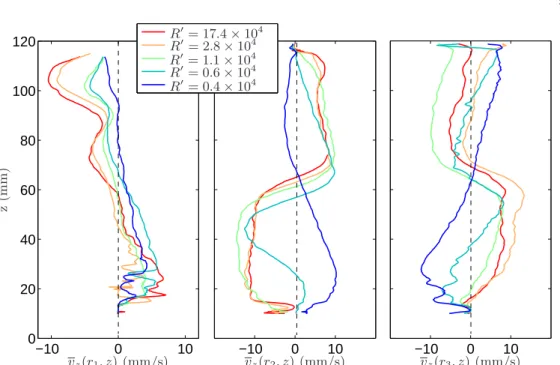
We focus here on the topology of the secondary flow. In order to do so, vz(r, z) is measured

at the three radii r1, r2and r3. Figure 4 represents time averaged vz(r1, z), vz(r2, z) and

vz(r3, z) profiles for 5 different R′ values ranging from 0.4 × 10 4

to 2.8 × 104

. Note that as the probes are situated at the bottom of the channel pointing in the upward direction, when vz> 0 the flow is going up. Measurements at r2and r3 reveal the existence of two

different types of velocity profiles, when R′ _{is changed.}

For R′ _{60.5 × 10}4

, in the lower half of the device, the fluid is going downward in the middle of the gap and upward along the inner and the outer walls. Symmetrically, in

−10 0 10 −10 0 10 0 20 40 60 80 100 120 −10 0 10 vz(r1, z) (mm/s) vz(r2, z) (mm/s) vz(r3, z) (mm/s) z (m m ) R′_{= 17.4 × 10}4 R′_{= 2.8 × 10}4 R′_{= 1.1 × 10}4 R′_{= 0.6 × 10}4 R′_{= 0.4 × 10}4

Figure 4. vz(r, z) profiles for different R′. On the left, we display the mean profiles at

r1= 16 mm, in the middle the ones at r2= 25 mm, and on the right the ones at r3= 34 mm.

Colors encode the five tested Hartmann numbers according to the legend. The high frequency spatial structures correspond to systematic noise, see text for details.

the upper half, the fluid flows upward in the middle of the gap and downward along the inner and the outer walls. The comparison with the numerical studies by Vantieghem & Knaepen (2011) and Zhao & Zikanov (2012) suggests the following interpretation. In their square duct aspect ratio, they found a secondary flow that consists of two pairs of large counter-rotating vortices, one pair near the inner wall and the other near the outer. In their simulations, the two vortices in the lower part of the duct have the same circulation sense, opposite to that of the two in the upper part. This configuration is compatible with the axial velocity profile at R′ _{60.5 × 10}4

presented in figure 4, if the vortex centers are located between r1and r2for the inner vortices and beyond r3 for the

outer vortices. This configuration is also compatible with the mechanism of generation of the Dean secondary flow due to inertial forces in a curved channel. Indeed, in these flows, the pressure gradient induced by the curvature is not balanced by the centrifugal force in the boundary layer, then it produces an inward flow at the top and bottom of the channel.

For R′ _{≈ 1 × 10}4

, vz(r2, z) and vz(r3, z) change drastically while vz(r1, z) does not. In

this case, in the lower half of the device, the fluid is going downward near the inner wall and in the middle of the gap and it is going upward near the outer wall. Symmetrically, in the upper half, the fluid is going upward in the middle of the gap and downward along the inner and the outer walls. This would suggest that the magnetic field shifts the mean position of vortices centers toward the outer wall. They would then be located between r2 and r3 for the inner vortices, squeezing the outer vortices close to the outer

wall. Nevertheless, according to simulations by Vantieghem & Knaepen (2011); Zhao et al.(2011); Zhao & Zikanov (2012) it is likely that this observation of the mean flow traces back to a change in the secondary flow dynamics. In section 5, we will address the

10

10

0.25

0.5

0.75

-0.1

-0.05

0

0.05

0.1

Figure 5.Intensity of the normalized axial velocity profile measured at r2 vz(r2, z)/U0 in the

(R′_{, z)-plan smoothed over a window of size ∆z = 2 mm. The dot-dashed line at R}′_{= 0.5 × 10}4

represents the topological change in the mean flow.

dynamical aspects of this transition.

In order to underline that the topological change is controlled by R′_{, we represent the}

vz(r2, z)/U0 profiles (encoded in color) as a function of z and R′ in figure 5. Despite

some noisiness around R′ _{≈ 5 × 10}3

(dot–dashed line) where the transition occurs, the secondary flow topology evolution is well ordered by R′ _{that appears as a good control}

parameter for this transition. Observing the figure from large to small R′_{, we see that the}

amplitude of the secondary flow is rather stable for R′ _{going from 2.5 × 10}5

to 1.5 × 104

. Below R′ _{= 1.5 × 10}4

, the secondary flow shrinks and the extrema shift close to the center of the cell. It is only below R′ _{= 5 × 10}3

that the direction of the time averaged flow measured by the probe changes. We focus on the origin of this transition in the next section.

4.2. Spatial fluctuations of the mean secondary flow and the signature of the ”magnetic” regime

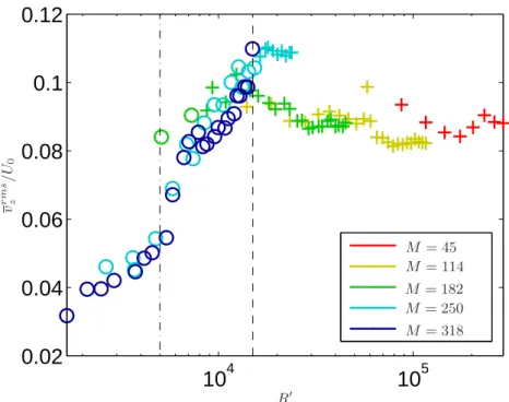
As mentioned in section 4, in figure 5 we observe a shrink of the vz(r2, z)/U0amplitude for

R′ _61.5×104

followed by a change of sign in the axial velocity. To quantify this shrink of the secondary flow, we compute the spatial root mean square of the mean velocity profile vrmsz (r = r2)/U0 displayed in figure 6 as a function of R′. This represents the secondary

flow amplitude normalized by the scaled azimuthal velocity. As we perceived previously, the secondary flow amplitude increases from 4% for small R′ _{to a maximum of 10% of}

the azimuthal velocity at R′_{≈ 1.5 × 10}4

. Beyond this value the amplitude stabilizes to values of order 8 − 9%. It is well known that high magnetic fields,corresponding to low R′ _{bidimensionnalise conducting liquid flows (Moreau (1990)). In our case, it implies a}

10

10

0.02

0.04

0.06

0.08

0.1

0.12

Figure 6.The amplitude |v|z(r2) normalized by the scaling of the azimuthal velocity U0along

R′_{. Crosses refer to the cases H}′_{/△r > 1 called ”hydrodynamic”regimes and circles correspond}

to H′_{/△r 6 1 named ”magnetic” regimes. Colors correspond to different Hartmannnumbers.}

Secondary flow behavior thus shows the existence of two regimes: at high R′_{, where}

inertial terms dominates magnetic force, the secondary flow amplitude directly depends on the mean azimuthal velocity. We will refer to this case as ”hydrodynamic” regimes. At low R′ _{that we will associate to ”magnetic” regimes, the amplitudes of the secondary}

flow are drastically reduced and decrease faster than the azimuthal flow.In figure 6, we marked as ◦ regimes where H′ _{issmaller than△r and as + regimes where H}′ _{is greater}

than △r. We can see that all the H′_{/△r 6 1 values are situated in the part of the curve}

where the amplitude of the secondary flow decreases. Therefore, this confirms that, in the so-called ”magnetic” regime, the relevant length for velocity gradients is H′_{. While}

when H′_{/△r > 1, the gap △r where centrifugal effects take place, becomes the relevant}

length. As both R′_{(I, B) and H}′_{(I, B) are biunivocal functions, this onset can be placed}

around R′ _{≈ 1.5 × 10}4

in our experiment (marked by the dash line in figure 6 where we also report the dot-dash line at R′ _{≈ 5 × 10}3

which corresponds to the change of sign in the time averaged velocity of figure 5). This limit also corresponds to a drop in the secondary flow amplitude showing again that this change may be associated with another transition between two regimes.

5. Dynamical measurements

5.1. Spectral analysis

In this section, to characterize the dynamical properties of the transition at H′_{/△r = 1,}

we will rely on type II runs described in 2. We only focus on the probe at r = r2. To

get a better insight of the transition, 2000 profiles are recorded consecutively with time sampling from ∆t ≈ 0.2 s to ∆t ≈ 0.04 s for faster regimes. These longer measurements

0

0.5

1

1.5

2

2.5

3

0

0.5

1

1.5

2

2.5

3

3.5

4

Figure 7. Temporal power spectral density. It is calculated in each axial sample probed by the the US sensor and averaged over a spatial window z ∈ [20, 100] mm. Five differentR′ _are represented. Spectra are shifted for clarity. The colored areas distinguish: in red, the lowest frequency mode, named excursion; in yellow, the tilted mode 1; in green, the tilted mode 2; in blue, the high frequency regime dominated by the noise.

allow us to resolve low frequency modes. In figure 7, we report power spectral density (PSD) for different R′_{. The PSD plotted in figure 7 are obtained as follow. The PSD}

in time is computed at each point along the z axis located between 20 and 100 mm and then these PSD are averaged together. In the figure, they are vertically shifted to improve clarity and the frequency is non-dimensionalised by the azimuthal rotation frequency (frot= U0/(2π¯r)). Starting from the PSD at the lowest R′= 0.2 × 10

4

, we can distinguish four regions and three distinct peaks:

• The region below 0.2 frotcolored in red on figure 7, contains a low frequency mode

that we call excursion for a reason that will be clarified in the discussion of section 6. For R′_{= 0.2 × 10}4

this is the most powerful peaks.

• A second peak is included in the region between 0.2 frot and 0.7 frot (in yellow in

figure 7). We called the corresponding tilted mode 1.

• A smaller peak appears between 0.7 frotand 2 frot(in green in figure 7). This mode

is named tilted mode 2 in the following.

• The last region (in blue on figure 7) does not contain peaks any more but reveals the level of the background velocity fluctuations.

This mode identification relies on the study of space-time diagrams as the ones shown in fig. 9 and on the corresponding time correlation function as the ones reported in fig.10. At R′ _{= 0.2 ×10}4

most of the energy is concentrated in the 3 peaks while it is much more distributed for higher R′_{. Nevertheless the previous segmentation remains valid at higher}

R′ _{although the relative energy contained in each region evolves. The background noise}

10

10

0

0.1

0.2

0.3

0.4

0.5

Figure 8.Integration the PSD for 4 different domains and normalized by the whole spectrum integral. Each domain corresponds to a dynamical mode : f < 0.2frotis the excursion mode ( ),

0.2frot< f < 0.7frot is the tilted mode 1 (⋆), 0.7frot< f < 2frot is the tilted mode 2 ♦), and

2frot< f corresponds to the high frequency fluctuations +). From left to right: the dot-dashed

line at R′_{= 0.5 × 10}4

corresponds to the topological change of the mean flow (cf figure 5 , the dashed line at R′_{= 1.5 × 10}4

corresponds to the fluctuations reduction threshold observed on figure 6, the dot-dashed line at R′_{= 2.5 × 10}4

corresponds to the maximum amplitude of the tilted mode 1 and the last dashed line at R′_{= 3 × 10}4

, where the tilted mode 1 starts to decay, corresponds to the balance H′_{= H/2.}

we observed –as expected– a similar tendency with H′_{/△r (not shown), without being}

able to determine if this number provides better description.

In order to quantify the relative weight of theses modes, we extract the evolution of their relative energy in each region as a function of R′_{. This is done by integrating the PSD}

within the 4 different domains (f < 0.2frot, 0.2frot < f < 0.7frot, 0.7frot < f < 2frot,

2frot < f ) and by dividing it by the total energy of the spectra. Note that the results

hardly depend on the exact values chosen for the limiting frequencies. In figure 8 we report the modes contribution along R′_{. First, as expected, the proportion of the high}

frequency fluctuations, depicted by the blue crosses, remains almost constant with R′_and

so they are probably due to higher frequency incoherent fluctuations or to measurement noise. The lowest frequency mode amplitude, depicted by the red circles, decreases when R′ _{is increased until R}′ _{= 1.5 × 10}4

which also corresponds to H′_{/△r = 1. It prevails}

at small R′ _{up to R}′ _{= 0.5 × 10}4

corresponding to the left dot-dashed line. Above R′ _{= 1.5 ×10}4

, it remains nearly constant. The two other modes amplitudes (depicted by the yellow stars and the green diamonds for the Titled mode 1 and 2 respectively) start to grow and dominate around R′ _{= 0.5 × 10}4

. The tilted mode 2 reaches its maximum around R′_{= 10}4

whereas the tilted mode 1 grows until R′_{∼ 2 × 10}4

and decreases above R′ _{= 3 × 10}4

. This last value coincides with values of the driving parameter around H′ _{= H/2 (shown by the right dashed line). Above this value, at higher R}′_{,the free force}

Figure 9.Spatiotemporal diagram of vz(r2, z, t) along the dimensionless time t = τ frot. From

left to right: R′_{= 2.3 × 10}4

, R′_{= 0.8 × 10}4

and R′_{= 0.3 × 10}4

. The color map is [−60, 60] mm/s for the two graphs on the left, and it is reduced to [−20, 20] mm/s for the right one. The red (resp. the blue) corresponds to positive (resp. negative) vz(r2, z, t) values. On the left, structures are

moving from the covers toward the duct center. In the middle, these structures are destabilized by a low frequency mode. On the right, the low frequency mode which corresponds to slow excursions of positive or negative vz(r2, z) is observed.

bulk definition we used becomes irrelevant. The tilted mode 1 remains the dominant mode until R′ _{= 10}5

. Above this value of R′_{, the energies of the regions with peaks are coming}

from the background velocity fluctuations.

We have represented by vertical lines in figure 8 the different transitions mentioned above. From these observations, one may interpret the different regimes as follow. At high R′_and

H′ _{the Lorentz force acts as would do the pressure gradient in the Dean configuration. At}

such large Reynold numbers, the flow is highly fluctuating. When R′ _{is decreased and H}′

becomes of order of H/2 inductive effects start to act and attenuate the fluctuations. The tilted mode 1clearly becomes dominant in this regime. When R′ _{is further reduced, H}′

becomes the smallest scale of the problem and the magnetic effects prevail and reduce the fluctuations. In the following we will focus on describing the different dynamical modes we have extracted in order to get their characteristics and relate them to the different thresholds we captured.

5.2. The dynamical modes characterization

Figure 9 gathers the spatiotemporal diagrams of the axial velocity for 3 different R′

values. Time is normalized by the rotation frequency as t = τ frot. For the highest R′

value (left graph), structures, corresponding to the titled mode 1, drift from the top and bottom covers to the duct center. These structures consist of alternative positive and negative axial velocities with a greater intensity in the upward direction in the upper part of the duct and in the downward direction in the lower part of the duct. Their axial wave number is k = 2π/H. When R′ _{decreases, the structures are destabilized and}

their propagation is blurred as can be seen in the central panel of figure 9. In addition, low frequency modulations appear. In this particular regime (R′ _{= 0.8 × 10}4

), there is coexistence of the three dynamical modes as we can see in figure 8. Finally for smaller R′ _{values (right panel) the amplitude of the flow is divided by 3 (for readability the}

colorbar has been changed). Propagative structures are not present any more. Instead, larger structures, evolving on long time scales without any axial propagation nor any noticeable periodicity, are observed. This is why we refer to this mode as the excursion

Figure 10.Time correlation function hv(δz, t)i along the dimensionless time t = τ frot.From

left to right: R′_{= 2.3 × 10}4

the tilted mode 1, R′_{= 0.8 × 10}4

combination of tilted mode 1, tilted

mode 2 and excursion mode, R′_{= 0.3 × 10}4

excursion mode. The color map is [−0.2, 1] for all graphs.

mode mentioned previously.

To better characterize these structures, we calculate the normalized time correlation for different distance intervals δz between measurement points. As the primary structures are propagating toward the middle of the duct, we only calculate the normalized time correlation over z ∈ [z1= 20 mm, z2= 70 mm]: hv(δz, τ)i =_N1 1 X N v′_{(z, τ )v}′_{(z + δz, τ )} v′_{(z, τ )}2 , (5.1)

where τ = t · frot is the dimensionless time, v′(z, τ ) = v(z, τ ) − hv(z, τ)i is the axial

velocity fluctuations, N = (z2− z1)/δz is the number of intervals we can extract in

the region of interest. The 2D autocorrelation functions presented in figure 10 confirm the first observations made about the spectra of figure 7. At high R′ _{(typically larger}

than 105

, not shown), structure amplitudes are small compared to the noise level and are hardly visible. The structure amplitudes grow when the R′ _{decreases and get clearly}

visible over the noise background as illustrated in the left panel of figure 10. For even lower R′_{,half period structures and a low frequency modulation appear as illustrated in}

the central panel. Finally the initial structures disappear completely and only the low frequency mode subsists (right panel of figure 10). This observation confirms results of figure 8, i.e. there are several exchanges of the predominant mode controlled by either H′

or R′ _{that lead to a reduction of the secondary flow and to a change of sign in the axial}

velocity. When the tilted modes become dominant (1.5 × 104

6 R′ ₆₁₀5

), the phase velocity of the waves in dimensionless unit (given by the slope of the structure in fig-ure 10) is stable with R′_{. It means that the dimensional phase velocity is proportional to}

U0. In addition, whatever the azimuthal velocity, since the axial wave number is around

kH = 2π, the period is around T = 2/frot. This tends to prove that the corresponding

structures are actually only advected by the mean flow.

To investigate the level of noise on the dynamical modes, we estimate the contrast of the pattern in figure 10. It can be obtained from the value of the first minimum of the normalized auto-correlation function in time 5.1 taken at ∆z = 0. These values are rep-resented as a function of R′ _{in figure 11 where we can see the presence of a minimum}

around R′ _{≈ 2.4 × 10}4

fig-10

10

−0.4

−0.3

−0.2

−0.1

0

0.1

0.2

0.3

Figure 11.Minimum of the normalized self-correlation function in time for different R′ _{as a}

measure of the contrast of the wavy pattern. The blue crosses identify the minimum of each run. Circles are locally averaged values with error bars standing for the local dispersion. The dash-dotted lines correspond to some of the thresholds displayed in figure 8. See text.

ure 10 and to the maximum of the tilted mode 1 contribution represented in figure 8. For R′ _{>2.4 × 10}4

the evolution does not present any clear tendency. However, below R′ _{≈ 5 × 10}3

, the value of the first minimum is no longer negative. This is due to the superposition of the lowest frequency mode (excursion mode) and the higher frequency modes (titled modes) in the correlation function. Below this point the fast oscillations are not intense enough compare to the slow oscillations to generate a negative first minimum in the correlation function. This fact confirms that the excursion mode is predominant below this point.

6. Discussion

Regarding our results and previous studies, it seems that we observe two different dynamical modes taking place respectively at low and moderate R′_{. In this section we}

compare our measurements to numerical studies of such forcing, especially Zhao et al. (2011) and Zhao & Zikanov (2012). Even if both used cells with aspect ratio different from our –infinite cylinders in Zhao et al. (2011) and square duct in Zhao & Zikanov (2012)– they worked in the same range of parameters. According to their geometry, their range of Reynolds and Hartmann layer thickness, one can evaluate BaN−2 > 1,

R′ _{∼ 1500 and H}′_{/△r ∼ 0.15 in the infinite annular configuration of Zhao et al. (2011)}

and BaN−2610−2, R′∼ 1.8 × 104and H′= H/4 in the square duct of Zhao & Zikanov

(2012). In the former configuration, i.e. when the conductive fluid is confined between two infinite concentric cylinders, axisymmetric perturbations consisting of counter-rotating

Figure 12.Schematic cut of the cell with a sketch of the mechanism involved in the tilted modes. The ellipses represent the stretched vortices and the gray area represents the volume investigated by the probe. Each right curve represents the corresponding velocity profile measured by the probe. The outer vortex is tilted in radial direction with a positive angle in the bottom part and a negative angle in the top part. The vortex is created in the bulk, then its center shifts toward positive r-direction. Then vortices intensity decreases and they disappear near the outer cylinder.

toroidal vortices concentrated in the outer half of the channel are observed. The vortices are elongated in the axial direction due to the influence of the magnetic field which tends to suppress velocity gradients in its direction. Moreover, as the vortices are arranged side by side in the radial direction, they have elliptic shapes. The large axes of these ellipses are close to the magnetic field direction with slightly tilted angle toward the r-direction. A key point here is that the counter-vortices have two possible orientations, thus, the tilt angle can either be positive or negative. The Lorentz and centrifugal forces equally contribute to the two angle configurations and the selected mode depends on the initial conditions. Zhao et al. (2011) also found that these modes present time oscillations. The dynamics involves the creation of a new vortex in the inner part of the channel whose center shifts in the positive r-direction and whose amplitude grows. Finally, the vortex intensity decreases and vanishes near the outer cylinder. This leads to the general shift of all vortices. For more details see Zhao et al. (2011).

This secondary flow is compatible with the structure dynamics of the titled mode re-ported in the previous sections. Indeed if we project the velocity created by the tilted vortices along the cylinder axis, the combination of the center shift in the positive r-direction and the tilt would produce the pattern we observe in the left panel of figure 9. As the forcing has a mirror symmetry with respect to the mid-plan normal to ~ez, we

ex-pect that the flow resex-pects this symmetry. Therefore the vortices in the upper and lower part of the duct must be tilted with opposite angles. Whatever is the tilted angle, the

vortices centers always shift toward the positive r-direction, therefore the sign of the tilt angle determines the sense of propagation of the structure we observe. Vortices rotating in the clockwise direction would create structures propagating in the downward direction, while those rotating in the anticlockwise direction would create structures propagating in the upward direction. This explains why we observe structures going in opposite sense (from the covers to the center of duct).

In figure 12, we report the schematic evolution of the time oscillation of the vortices network and its consequences on the axial velocity measurements obtained by the probe at r2. As mentioned above, between infinite cylinders the tilt angle sign is determined

by initial conditions. However, here the presence of top and bottom boundaries could remove the degeneracy of the system and force a tilt angle. Therefore, depending on the duct aspect ratio and on the Hartmann number opposite tilt angles can be observed. This ascertainment is reinforced by the results of Boisson & Aumaitre (2012) who, at moderate Hartmann number and in a smaller aspect ratio, observed travelling waves emerging from the duct center and going toward the top and bottom boundaries. In this system the vortices would be tilted in a symmetrical manner than the one we presented in figure 12. This is compatible with the hypothesis that the duct geometry could in-fluence the secondary mode topology. Another point that supports this assumption, is the fact that the thickness of the inertial magnetic layerH′ _{is about half the height of}

the cell (H/2) at the maximum of predominance of the titled modes. Supposing that the tilted mode wavelength is determined by H′_{, the matching between those and the}

axial characteristic length would favor the emergence of the mode. In this description the tilted mode would be characteristic of small aspect ratio devices. Nevertheless we observed a discrepancy with the numerical results of Zhao et al. (2011) concerning the oscillation period. Indeed they found a period an order of magnitude larger than the one we actually observe. This could be due to the different aspect ratios which would modify the dynamics. Moreover we observed that the frequency oscillation is ∼ 0.5frot in the

parameter range where these titled modes prevail, thus is growing linearly with Re in contrast to the low frequency that Zhao et al. (2011) estimated. That is why we con-clude that the vortices shift we observed is somehow induced by the mean flow advection leading to a smaller period and a linear dependence on Re.

The low frequency mode –so-called the excursion mode– represented in the right panel of figure 9 corresponds to excursions of positive velocity from the lower part to upper part of the duct (from t ≈ 20 to t ≈ 30) and the opposite (from t ≈ 30 to t ≈ 40). That is to say to the expansion of one of the two large vortices near the outer wall and its drift toward the opposite half of the duct. These slow events are accompanied by the growth of the kinetic energy and end by its decrease. This corresponds very well to the description of the first axisymmetric instability Zhao & Zikanov (2012) found numeri-cally in a square duct. We have observed these excursion modes, for Re = 17000 with our definition which corresponds to half the threshold given by Zhao & Zikanov (2012). However, as the present aspect ratio is greater than that of the square section, a different threshold is not necessarily surprising. The dimensionless duration of these slow events is approximately τ = 30, which is less but of the same order of magnitude than the one calculated by Zhao & Zikanov (2012) and that corresponds to the low frequency peak we observed in the figure 7. Therefore we can assume that the low frequency mode we captured corresponds to the first axisymmetric instability described in Zhao & Zikanov (2012). Our interpretation of the apparition of these excursion modes is related to the inertial magnetic layerbeing smaller that the gap. In these regimes the competition be-tween the geometrical effects favoring structures with characteristic lengths of the order of △r and the induction effects generating structures at the smaller length H′_{. Then, we}

Figure 13.Scheme of the mechanism involve in the excursion mode. The outer vortex inflates in the z-direction and r-direction. This low frequency contribution generates the change of sign in the time averaged profiles that we represented in figures 4 and 5.

could assume that the adaptation of the magnetic structures to the cell would create the excursion mode until it can actually fit the geometry. In this description the excursion mode would be characteristic to small aspect ratio devices.It has to be noted that the numerical simulations of Zhao & Zikanov (2012) were performed at much lower BaN−2

values that here. However, we only observe excursion modes for high Hartmann numbers, that is to say for the lower part of our BaN−2 range where the inertial effects begin to

be weak.

7. Conclusion

In this paper we have presented experimental results obtained in η = O(1) aspect ratio duct forced electromagnetically at moderate Hartmann numbers.In most of our regimes, the inertial effects cannot be neglected.It constitutes a step toward the understanding of the mechanisms in action when a magnetic field yields to 2D flows of conducting fluids. The measurements were performed using ultrasound probes at different angles and different radial positions. First we proposed a scaling for the azimuthal velocity which depends on the product between the electric current and the magnetic field suggesting that the current is not restricted to the Hartmann layer. Therefore, we constructed an intermediate layer, H′ _{–named the inertial magnetic thickness– that depends on the}

electric current and on the magnetic field where the electric currentis concentrated. This layer is larger than the laminar Hartmann layer. We suggest that this characteristic length controls the flow structure. Therefore, we propose that the inertial magnetic thickness we introduced in this article could be applied to all kinds of MHD flow regimes at

tilted mode 1 tilted mode 2 excursion mode H′_{/△r = 1 H}′_{/(H/2) = 1 H}′ R′_{≈ 5 × 10}3 R′_{≈ 1.5 × 10}4 R′_{≈ 2.4 × 10}4 R′ H y d ro d y n a m ic M a g n et ic

Figure 14.Diagrammatic sketch of the transitions involved in the experimental setup as func-tion of the pertinent control parameter R′ _{and the characteristic length scale H}′_{, the inertial}

magnetic layer.

moderate Hartmann numbers andwhere the inertial effects cannot be neglected, as the controlling parameter of the dynamics. The Reynolds number R′ _{constructed from H}′

coincidently have the same I and B dependencies than the one introduced by Moresco & Alboussiere (2004) even if the latter relied on a balance between the Lorentz force and viscous dissipation while in our case inertial terms are used to balance the Lorentz force. To establish our scaling, we have assumed the existence of a force-free bulk where the induced current are proportional to σU0B. This assumption seems corroborated by our

results that present clear transitions controlled by H′ _{and R}′_{. Nevertheless an explicit}

test would require measurement of the azimuthal velocity field which is clearly out of reach in the present geometry.

Our work suggests thatthe time averaged secondary flow is composed of two sets counter-rotating vortices arranged radially. We also observe a transition between two regimes of the secondary flow. They seem controlled by both H′_{, theinertial magnetic thicknessand}

R′ _{–a Reynolds number based on H}′_{. The flow topology in the second regime is difficult}

to determine directly from the time averaged measurements, however our dynamical studies suggest a probable scenario. The magnetic field diminishes velocity gradients in its direction (the axial direction) while inertial forces enlarge these gradients in the radial direction. For large R′ _{(high centrifugal force), we measure the recirculation induced by}

the inner vortices. This recirculation scales with the Reynolds number, while in the ”magnetic” regime it varies nonlinearly with respect to the Reynolds number.

This means that the magnetic field reduces velocity gradients in its direction. For small R′ _{(high magnetic field), the secondary flow in the middle of the duct has a very small}

contribution to the time averaged secondary flow. The excursion of the outer vortices characterizing the first axisymmetric instability described by Zhao & Zikanov (2012) seems responsible for the change of sign we observed on the time averaged mean flow. Finally, the first dynamical mode we observe must be vortices tilted in the radial direc-tion and advected by the mean flow. These vortices present in the unbounded cylinder calculations of Zhao et al. (2011) travel radially and give birth to the axial velocity waves observed here and in Boisson & Aumaitre (2012). Depending on the tilt angle, we can observe a propagation in the sense z > 0 or z < 0. The tilted modes seem to be enhanced when the inertial magnetic layer thickness is between the gap width and half the cell height in such a way that the magnetic effects match the centrifugal and inertial effects in this geometry. When the inertial magnetic layeris increased further, the induction cancels out and the magnetic strength cannot sustain these structures out of the 3D turbulent fluctuations any more. As a contrary to excursion mode the relevant dimension is the cylinder height in this mode. Therefore, as we have summarized in

fig-ure 14, we have attributed the presence of these two dynamical modes to the experiment aspect ratio which shares geometrical features with the infinite cylinder but also with the square section duct depending on which geometric characteristic length matches the inertial magnetic layerthickness.As mentioned before our aspect ratio and the range of parameters we explored are somehow different from the ones of Zhao et al. (2011); Zhao & Zikanov (2012). A more accurate comparison would require dedicated simulations that could actually also be used to validate the existence of a force-free bulk.

The authors would like to thank L. Cherfa, V.Padilla for their help in the experimental design, the laboratory PhotoRB for its help on the first visualisation process, Y. Bertrand and O. Cadot for helpful discussions. We also would like to thank the anonymous review-ers for their constructive comments, which helped us to improve the manuscript.

REFERENCES

Baylis, JA 1964 Detection of the onset of instability in a cylindrical magnetohydrodynamic flow. Nature 204, 563.

Baylis, J. A.1971 Experiments on laminar flow in curved channels of square section. Journal of Fluid Mechanics 48 (03), 417–422.

Baylis, J. A. & Hunt, J. C. R.1971 Mhd flow in an annular channel; theory and experiment. Journal of Fluid Mechanics 48, 423–428.

Boisson, J., Klochko A. Daviaud F. Padilla V. & Aumaitre, S.2012 Travelling waves in a cylindrical magnetohydrodynamically forced flow. Physics of Fluids (1994-present) 24 (4), 044101.

Brito, Daniel, Nataf, Henri-Claude, Cardin, Philippe, Aubert, Julien & Masson, Jean-Paul 2001 Ultrasonic doppler velocimetry in liquid gallium. Experiments in fluids 31_{(6), 653–663.}

Chandrasekhar, S.2013 Hydrodynamic and hydromagnetic stability. Courier Corporation. Digilov, R. M.2007 Making a fluid rotate: Circular flow of a weakly conducting fluid induced

by a lorentz body force. American Journal of Physics 75 (4), 361–367.

Duran-Matute, M, Trieling, RR & van Heijst, GJF2011 Scaling and asymmetry in an electromagnetically forced dipolar flow structure. Physical Review E 83 (1), 016306. Eckert, S. & Gerbeth, G.2002 Velocity measurements in liquid sodium by means of

ultra-sound doppler velocimetry. Experiments in Fluids 32 (5), 542–546.

Hunt, JCR & Stewartson, K1965 Magnetohydrodynamic flow in rectangular ducts. ii. Jour-nal of fluid mechanics 23 (03), 563–581.

Khalzov, IV, Smolyakov, AI & Ilgisonis, VI2010 Equilibrium magnetohydrodynamic flows of liquid metals in magnetorotational instability experiments. Journal of Fluid Mechanics 644_{, 257–280.}

Krasnov, DS, Zienicke, Egbert, Zikanov, Oleg, Boeck, Thomas & Thess, Andre2004 Numerical study of the instability of the hartmann layer. Journal of Fluid Mechanics 504, 183–211.

Mikhailovich, B, Shapiro, A, Sukoriansky, S & Zilberman, I2012 Experiments with tur-bulent rotating mhd flows in an annular gap. Magnetohydrodynamics (0024-998X) 48 (1). Moffatt, H. K.1978 Field Generation in Electrically Conducting Fluids. Cambridge University

Press, Cambridge, London, New York, Melbourne.

Moreau, R. J.1990 Magnetohydrodynamics, , vol. 3. Springer Science & Business Media. Moresco, P. & Alboussiere, T.2004 Experimental study of the instability of the hartmann

layer. Journal of Fluid Mechanics 504, 167–181.

Poth´erat, A2012 Three-dimensionality in quasitwo-dimensional flows: Recirculations and bar-rel effects. EuroPhysic Letters 98, 64003.

Poth´erat, Alban & Klein, Rico2014 Why, how and when mhd turbulence at low becomes three-dimensional. Journal of Fluid Mechanics 761, 168–205.

Sommeria, J & Moreau, RJ 1982 Why, how, and when, mhd turbulence becomes two-dimensional. Journal of Fluid Mechanics 118, 507.

Stelzer, Zacharias, C´ebron, David, Miralles, Sophie, Vantieghem, Stijn, Noir, J´erˆome, Scarfe, Peter & Jackson, Andrew2015a Experimental and numerical study of electrically driven magnetohydrodynamic flow in a modified cylindrical annulus. i. base flow. Physics of Fluids (1994-present) 27 (7), 077101.

Stelzer, Zacharias, Miralles, Sophie, C´ebron, David, Noir, J´erˆome, Vantieghem, Stijn & Jackson, Andrew2015b Experimental and numerical study of electrically driven magnetohydrodynamic flow in a modified cylindrical annulus. ii. instabilities. Physics of Fluids (1994-present) 27 (8), 084108.

Tabeling, P. 1982 Sequence of instabilities in electromagnetically driven flows between con-ducting cylinders. Physical Review Letters 49 (7), 460.

Tabeling, P. & Chabrerie, J. P. 1981 Magnetohydrodynamic taylor vortex flow under a transverse pressure gradient. Physics of Fluids (1958-1988) 24 (3), 406–412.

Vantieghem, Stijn & Knaepen, Bernard 2011 Numerical simulation of magnetohydrody-namic flow in a toroidal duct of square cross-section. International journal of heat and fluid flow 32 (6), 1120–1128.

Zhao, Yurong & Zikanov, Oleg2012 Instabilities and turbulence in magnetohydrodynamic flow in a toroidal duct prior to transition in hartmann layers. Journal of Fluid Mechanics 692_{, 288–316.}

Zhao, Yurong, Zikanov, Oleg & Krasnov, Dmitry2011 Instability of magnetohydrody-namic flow in an annular channel at high hartmann number. Physics of Fluids (1994-present) 23 (8), 084103.