Upper mantle anisotropy beneath the Geoscope stations

HAL Id: hal-01388830

https://hal.univ-reunion.fr/hal-01388830

Submitted on 27 Oct 2016

HAL is a multi-disciplinary open access

archive for the deposit and dissemination of

sci-entific research documents, whether they are

pub-lished or not. The documents may come from

teaching and research institutions in France or

abroad, or from public or private research centers.

L’archive ouverte pluridisciplinaire HAL, est

destinée au dépôt et à la diffusion de documents

scientifiques de niveau recherche, publiés ou non,

émanant des établissements d’enseignement et de

recherche français ou étrangers, des laboratoires

publics ou privés.

To cite this version:

Guilhem Barruol, Ruth Hoffmann. Upper mantle anisotropy beneath the Geoscope stations. Journal

of Geophysical Research : Solid Earth, American Geophysical Union, 1999, 104 (B5), pp.10757 - 10773.

�10.1029/1999JB900033�. �hal-01388830�

Upper mantle anisotropy beneath the Geoscope stations

Guilhem Barruol and Ruth Hoffmann

Laboratoire de Tectonophysique, CNRS, Université Montpellier II, Montpellier, France.

A b s t r a c t. Seismic anisotropy has been widely studied this last decade, particularly by measuring

splitting of vertically propagating core shear waves. The main interest in this technique is to

characterize upper mantle flow beneath seismic stations. On the other hand, the major restriction in

this method is that a single station gives a single anisotropy measurement. Alternative methods have

been developed in order to avoid this restriction. An accurate determination of upper mantle seismic

anisotropy beneath a seismic station may allow one, by doing anisotropy correction, to characterize

remote or deeper anisotropy. The Geoscope network is ideal for this purpose because it is composed

of a large set (about 26) of high-quality, broadband seismometers globally distributed and because

some of these stations have run for more than 10 years and most of them for more than 5 years. We

selected about 100 events at each site, generally of magnitude (mb) > 6.0, and we performed

systematic measurements of the splitting parameters (fast polarization direction

φ

and delay time

δ

t)

on SKS, SKKS, and PKS phases. Splitting on oceanic islands has been difficult to observe owing to the

low quality of the signal but also perhaps owing to complex upper mantle structures beneath the

stations. Station KIP (Kipapa, Hawaii) in the Pacific is the only oceanic Geoscope station with a clear

anisotropy. We determined well-constrained splitting parameters for 10 of the 17 continental stations

that may be explained by a single anisotropic layer. The poor correlation between fast polarization

directions and the absolute plate motion together with the apparent incoherence between the plate

velocities and the observed delay times suggest that a simple drag-induced asthenospheric flow alone

fails to explain most of the observations. For some stations located on or near major lithospheric

structures (TAM, Tamanrasset, Algeria, for instance), we observe a good correlation between fast

polarization directions and regional structures. At station SCZ (Santa Cruz, California), we found

clear variations of the splitting parameters as a function of the event backazimuth, compatible with

two layers of anisotropy. Three stations (CAN (Canberra), HYB (Hyderabad, India) and SSB (Saint

Sauveur Badole, France)) seem to be devoid of detectable anisotropy.

1. Introduction

Seismic anisotropy has become a fundamental tool to investigate the deep structure and deformation of Earth. Seismology and rock physics agree that seismic anisotropy in the lithosphere is almost ubiquitous and may be related either to rock microfracturing or to single crystal intrinsic elastic properties associated with crystal lattice preferred orientation. Upper mantle rock samples systematically show lattice preferred orientation, particularly of olivine, the major upper mantle component, that induce anisotropic seismic properties [Nicolas and Christensen, 1987]. This is well known from peridotite bodies outcropping in mountain belts [e.g., Peselnick et al., 1974] and in ophiolites [Christensen, 1978] and xenoliths brought up to the surface by volcanic or kimberlite eruptions [Boullier and Nicolas, 1975; Mainprice and Silver, 1993; Ji et al., 1994].

Shear wave splitting is directly induced by seismic anisotropy: A shear wave crossing an anisotropic medium splits into two perpendicularly polarized waves that propagate at different

velocities. The time lag (δt) between the two split wave arrivals

depends on the thickness and intrinsic anisotropy of the medium.

Copyright 1999 by the American Geophysical Union Paper number 1999JB900033.

0148-0227/99/1999JB900033$09.00

The azimuth (φ) of the fast split wave polarization plane is related

to the orientation of the structure. Since φ in upper mantle

peridotites is generally oriented close to the lineation direction [Mainprice and Silver, 1993], splitting of teleseismic phases such as S K S , SKKS and PKS has been used to characterize upper mantle flow. Most delay times obtained from SKS splitting lie in the range of 0.5-1.5 s, and the global average is around 1 s [Silver, 1996]. Intrinsic upper mantle rock S wave anisotropies lie in the range 2-5 % and therefore require a 100-300 km thick anisotropic layer [Mainprice and Silver, 1993] to account for the

observed δt.

The location of anisotropy along the path from the core-mantle boundary, where the upgoing S wave is generated, to the recording station is open to question because splitting could occur anywhere in the mantle. Seismological and petrophysical studies suggest that most of the anisotropy is restricted to the olivine stability field, i.e., above 410 km depth, in the lithosphere and/or asthenosphere [e.g., Fischer and Wiens, 1995; Karato et al., 1995; Meade et al., 1995]. The lithospheric and/or asthenospheric origin of shear wave splitting is still debated: The lithospheric origin of anisotropy is generally attributed to frozen-in deformation, related to past orogenies (see review by Silver [1996]). The asthenospheric anisotropy instead is related to sublithospheric upper mantle deformation induced by present-day plate motions [e.g., Bormann et al., 1996]. In the lower mantle, no evidence of anisotropy has yet been demonstrated but recent

Kendall and Silver, 1996; Garnero and Lay, 1997].

Typical delay times generated in the crust range from 0.1 to 0.2 s and could be related to microfracturing and to the state of stress in the upper crust [e.g., Crampin, 1984; Peacock et al., 1988] and/or to pervasive lower crustal fabric [e.g., McNamara and Owens, 1993; Herquel et al., 1995]. These values are in agreement with calculations of rock seismic properties suggesting

that δt up to 0.1 s per 10 km of crust may be observed [Barruol

and Mainprice, 1993]. Higher delay times, up to 0.5 s, were observed [Savage et al., 1990] but are exceptional. In summary, the crust may contribute to the splitting of vertically propagating shear waves, but in most cases, about 80% of the signal recorded by SKS waves have to be related to subcrustal anisotropy.

Splitting measurement of teleseismic shear waves such as SKS and SKKS waves is the easiest way to track the upper mantle anisotropy. Direct S phases may allow one to retrieve the anisotropy on the source-side of the path [Kaneshima and Silver, 1992] or, in some epicentral distance and event depths conditions, within the D" layer [Kendall and Silver, 1996; Garnero and Lay, 1997] but need to be corrected from the anisotropy beneath the station. Bouncing phases such as PS [Su and Park, 1994] or SS phases resulting from deep events may allow one to characterize the anisotropy at the bouncing point beneath Earth's surface [Wolfe and Silver, 1998]. Therefore a single station may potentially be used to get numerous anisotropy measurements at remote places where it is difficult to obtain a direct sampling from SKS splitting, such as the ocean basins, the subduction zones or the mountain belts, for instance. Obviously, the applicability of these new techniques depend on the reliability of the anisotropy correction underneath the station.

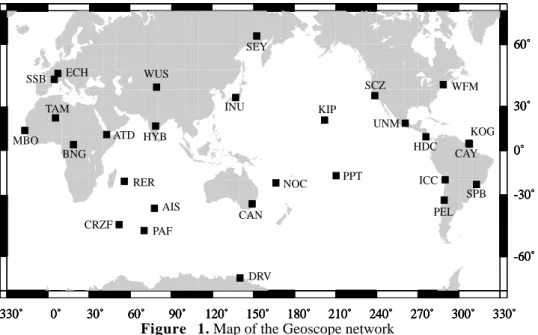
The aim of this study is to obtain the best possible estimate of the upper mantle anisotropy beneath the Geoscope stations from SKS splitting and to render possible future work requiring upper mantle anisotropy corrections. The Geoscope network, as most of the permanent global networks, is well suited for this purpose because it provides a large number (26) of high-quality, three-component broadband stations that are globally distributed (see locations in Table 1 and Figure 1). Most of the stations have operated for longer than 5 years and some for longer than 10 years.

In section 2, we describe our event selection and the results. In the section 3 we discuss the results with regard to already published measurements, the possible relationship between anisotropy and plate motions, the presence of several layers of anisotropy beneath some stations, the anisotropy beneath the oceans, the apparent upper mantle isotropy at three stations, and the relations between seismic anisotropy and some important geological structures. In the light of this discussion, we present the stations that can confidently be used for anisotropy correction.

2. Data and Results

We selected events of magnitude (mb) greater than 6.0 occurring at epicentral distances in the range 85° to 120°. For stations that operated for only a few years we lowered the magnitude threshold to 5.8, and for stations located in poorly illuminated areas we included events at distances up to 160°. The available data retrieved from the Geoscope jukebox generally yielded about 50-100 events fitting our criteria at each station.

The event origins and locations (Table A11

, available electronically) were taken from the U.S. Geological Survey

were computed using the IASP91 Earth reference model [Kennett, 1995].

Core shear phases (such as SKS, SKKS, or PKS) are generated through a P-to-S conversion at the core-mantle boundary and are initially radially polarized. Seismic anisotropy along the path of the upgoing SKS wave transfers part of the signal onto the transverse component. The shear wave splitting measurements were obtained using the Silver and Chan [1991] algorithm. This

method determines the anisotropy parameters, φ and δt, that best

remove the energy on the transverse component of the seismogram for a selected time window around the SKS phase. Typical SKS splitting measurements have already been described and analyzed elsewhere [e.g., Barruol et al., 1997b]. From the whole set of selected seismograms, more than 900 individual splitting measurements were performed at the 26 Geoscope stations. For each event the anisotropy parameters obtained are reported in Table A2, together with the phase used, the backazimuth of the event, and the error bars on the splitting

parameters from the 95% confidence interval in the (φ, δt)

domain. We finally ascribe a quality factor (good, fair, or poor) to the measurements depending on the signal to noise ratio of the initial phase, the correlation between the fast and slow split shear waves, and the linear polarization of the particle motion in the horizontal plane after anisotropy correction. This qualitative evaluation of the measurements is helpful for analyzing the final results. No systematic filtering were applied to the data. When necessary, they were band-pass-filtered (typically between 0.01 and 0.5 Hz) to remove high-frequency noise and long-period signal.

In simple anisotropic symmetry system the splitting parameters determined by the Silver and Chan [1991] method should not vary strongly with backazimuth. Systematic variations of the anisotropy parameters as a function of the event backazimuth or polarization direction and incidence angle may be used to detect differences between the model and the real geological structures, particularly the presence of several layers of anisotropy, heterogeneous anisotropy, and/or dipping axis of symmetry (see discussion below).

In some cases, we observe (Table A2) slight differences in anisotropy parameters deduced from SKS and SKKS phases from the same event. This could result from deep anisotropy within the D" layer: since SKS and SKKS phases emerge from the outer core at rather large distances from each other (about 700 km for epicentral distances of 100°), they do not cross the D" layer with the same angle of incidence [Kendall, 1997]. Assuming the D" layer is transversely isotropic with a vertical axis of symmetry, as suggested by Kendall and Silver [1996], or Garnero and Lay [1998], the SKS phase should cross the D" layer at near normal incidence angle, i.e., close to the isotropic direction, whereas the SKKS phase should cross the D" layer at a lower incidence angle and could be affected by the D" anisotropy.

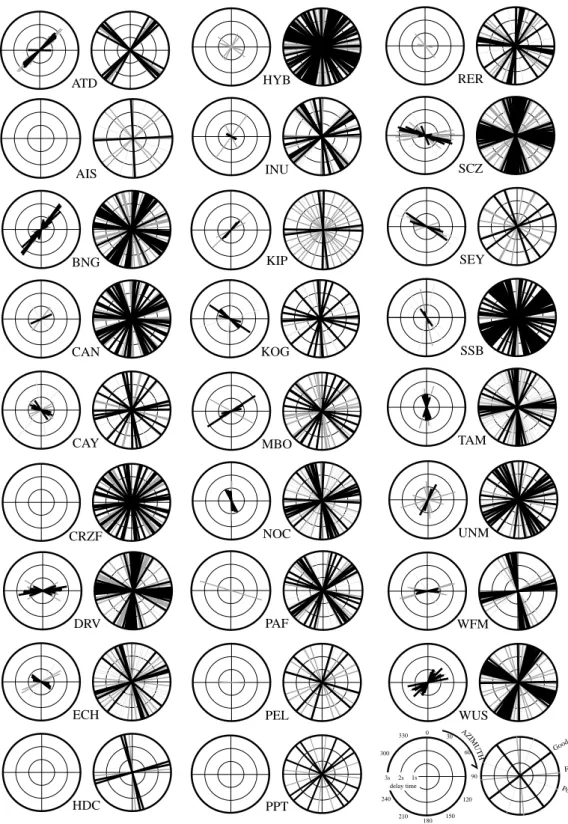
Figure 2 shows the results of the null and nonnull splitting measurements performed at each station, together with their quality. Null measurements (absence of splitting) may be explained either by an absence of anisotropy or by initial shear

1

Supporting data Tables (Tables A1 and A2) are available on diskette or via anonymous FTP from kosmos.agu.org, directory APEND (Username=anonymous, Password=guest). Diskette may be ordered from American Geophysical Union, 2000 Florida Avenue, N.W., Washington, DC 20009 or by phone at 800-966-2481; $15.00. Payment must accompany order.

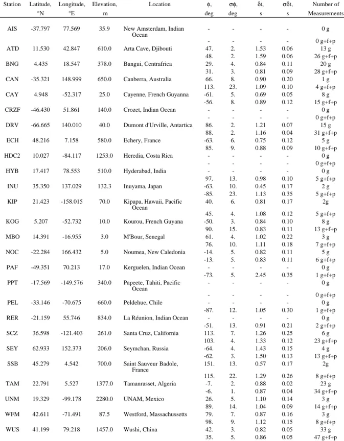
Table 1. Station Location and Mean Splitting Parameters With Their Error Bars Station Latitude, °N Longitude, °E Elevation, m Location φ, deg σφ, deg δt, s σδt, s Number of Measurements

AIS -37.797 77.569 35.9 New Amsterdam, Indian

Ocean

- - - - 0 g

- - - - 0 g+f+p

ATD 11.530 42.847 610.0 Arta Cave, Djibouti 47. 2. 1.53 0.06 13 g

48. 2. 1.59 0.06 26 g+f+p

BNG 4.435 18.547 378.0 Bangui, Centrafrica 29. 4. 0.84 0.11 20 g

31. 3. 0.81 0.09 28 g+f+p

CAN -35.321 148.999 650.0 Canberra, Australia 66. 8. 0.90 0.20 1 g

113. 23. 1.09 0.10 4 g+f+p

CAY 4.948 -52.317 25.0 Cayenne, French Guyanna -61. 5. 0.69 0.05 8 g

-56. 8. 0.89 0.12 15 g+f+p

CRZF -46.430 51.861 140.0 Crozet, Indian Ocean - - - - 0 g

- - - - 0 g+f+p

DRV -66.665 140.010 40.0 Dumont d'Urville, Antartica 86. 2. 1.21 0.07 15 g

88. 2. 1.16 0.04 31 g+f+p

ECH 48.216 7.158 580.0 Echery, France -63. 6. 0.75 0.12 5 g

85. 9. 0.88 0.09 10 g+f+p

HDC2 10.027 -84.117 1253.0 Heredia, Costa Rica - - - - 0 g

- - - - 0 g+f+p

HYB 17.417 78.553 510.0 Hyderabad, India - - - - 0 g

97. 13. 0.98 0.10 5 g+f+p

INU 35.350 137.029 132.3 Inuyama, Japan -63. 10. 0.45 0.17 2 g

-85. 23. 1.13 0.35 5 g+f+p

KIP 21.423 -158.015 70.0 Kipapa, Hawaii, Pacific

Ocean

40. 6. 0.81 0.17 2g

45. 4. 1.08 0.12 5 g+f+p

KOG 5.207 -52.732 10.0 Kourou, French Guyana -50. 3. 0.84 0.10 8 g

90. 15. 0.83 0.11 13 g+f+p

MBO 14.391 -16.955 3.0 M'Bour, Senegal 61. 4. 1.02 0.22 3 g

76. 10. 1.11 0.18 7 g+f+p

NOC -22.284 166.432 5.0 Noumea, New Caledonia -14. 5. 0.82 0.11 5 g

-13. 5. 0.83 0.11 6 g+f+p

PAF -49.351 70.213 17.0 Kerguelen, Indian Ocean - - - - 0 g

-73. 5. 2.45 0.35 1 g+f+p

PPT -17.569 -149.576 340.0 Papeete, Tahiti, Pacific

Ocean

- - - - 0 g

- - - - 0 g+f+p

PEL -33.146 -70.675 660.0 Peldehue, Chile - - - - 0 g

-87. 12. 1.05 0.30 1 g+f+p

RER -21.159 55.746 834.0 La Réunion, Indian Ocean - - - - 0 g

-51. 13. 0.91 0.21 2 g+f+p

SCZ 36.598 -121.403 261.0 Santa Cruz, California 113. 7. 1.26 0.25 6 g

103. 4. 1.33 0.12 23 g+f+p

SEY 62.933 152.373 206.0 Seymchan, Russia -64. 4. 1.43 0.15 4 g

-62. 3. 1.50 0.13 13 g+f+p

SSB 45.279 4.542 700.0 Saint Sauveur Badole,

France

151. 13. 0.57 0.17 2g

115. 22. 1.29 0.26 8 g+f+p

TAM 22.791 5.527 1377.0 Tamanrasset, Algeria -7. 2. 0.88 0.02 23 g

-6. 1. 0.87 0.04 34 g+f+p

UNM 19.329 -99.178 2280.0 UNAM, Mexico 26. 5. 1.10 0.14 3 g

89. 14. 1.04 0.09 14 g+f+p

WFM 42.611 -71.491 87.5 Westford, Massachussetts 79. 7. 0.87 0.16 3 g

98. 9. 1.12 0.15 8 g+f+p

WUS 41.199 79.218 1457.0 Wushi, China 42. 3. 0.82 0.05 33 g

35. 5. 0.86 0.05 47 g+f+p

The average values are calculated at each station using the good measurements only (g), then using the whole data set: the good (g), fair (f), and poor (p) splitting measurements. The number of individual measurements from which the average values are calculated is listed.

wave polarization parallel to the fast or slow polarization direction in the anisotropic layer. The large variability in the number of splitting measurements at each site is mainly due to the duration of recording period that varies from 2 years (KOG, for instance) to 12 years (SSB). The data quality also limits the number of usable events. In particular, few measurements were performed on oceanic island stations (see Figure 3) where sea waves introduce a strong background noise. Note that the value plotted for the nonnull measurements is the best value determined by the Silver and Chan [1991] program (see Table A2). In numerous cases, scattering of individual measurements appearing Figure 2 at some stations is not inconsistent but is related to

larger error bars in the φ-δt diagram.

Splitting parameters at each site were averaged using the method developed by Silver and Chan [1991], which weights

each individual nonnull measurement by its φ and δt error bars

(see Table A2). The mean splitting parameters reported in Table 1 and Figure 3 were first calculated from the good measurements only, then using the whole set of measurements (good, fair, and poor). This allows us to test the stability of the results and to sort the stations by measurement quality: (1) A first group of stations (ATD, BNG, DRV, NOC, SEY, TAM, and WFM) is characterized by consistent means obtained from the two different

data sets: φ and δt variations do not exceed ±5° and ±0.1 s,

respectively. The anisotropy at these stations can be qualified as very well constrained. (2) A second group of stations is characterized by variations in the calculated mean of more than

10° in φ and of more than 0.1 s in δt depending on whether only

good measurements or the whole measurements were used for the calculation. The anisotropy is therefore considered as "fairly" constrained. The dispersed values may either be related to complex deep structures (like perhaps at SCZ, KIP, WUS, and UNM) or to marginal measurements (like at CAY, ECH, INU, MBO, and KOG). (3) A third group of stations did not give good nonnull measurements (AIS, CRZF, HDC, PAF, PPT, PEL, and RER). The mean results calculated for these stations from the fair and poor measurements have to be considered as poorly constrained. Five of these stations are located on oceanic islands (see discussion below). The absence of good measurements obtained at the two continental stations of this group may be

explained by the small number of teleseismic events available (HDC and PEL). Station lying above subduction zones (INU, HDC, ICC, and PEL) did not give clear SKS splitting. This likely results from the complexity of the structure (several layers of anisotropy and dipping structures) that could be more efficiently solved by measuring local S wave splitting. (4) Finally, three stations seem to be devoid of anisotropy (CAN, HYB, and SSB). This conclusion is inferred by a good backazimuthal coverage of nulls (Figure 2). The apparent isotropy observed at these stations is discussed below.

3. Discussion

This discussion addresses the following points: First, we compare our measurements with previously published one. Second, we discuss the relationship between seismic anisotropy at the Geoscope sites and the corresponding plate motion vectors. Third, we test the presence of several layers of anisotropy at some continental stations where enough measurements are available (TAM, WUS, SCZ, and DRV). Fourth, we examine the anisotropy or the lack of anisotropy beneath the oceanic stations (RER, CRZF, PAF, and AIS in the Indian Ocean ; PPT and KIP for the Pacific). Fifth, we propose possible explanations for the apparent upper mantle isotropy observed at continental stations SSB, HYB, and CAN. Sixth, we finally discuss the relationship between geologic structures and seismic anisotropy at some well constrained stations: ATD and the Afar rift, ECH and the Hercynian Belt in France, NOC and the New Hebrides subduction zone, and finally SEY and the Verkhoyansk belt in northeastern Siberia.

3.1 Comparison With Previous Measurements

A decade ago, splitting measurements were already published for some Geoscope stations, mainly by Ansel [1989], Ansel and Nataf [1989] and Vinnik et al. [1989]. In the following, we briefly compare our results to the previous ones.

At AGD (the previous site close to ATD), Djibouti, Vinnik et al. [1989] found results (φ = N55°E, δt = 1.2 s) that seem

compatible with ours (φ = N47°E, δt = 1.53 s), except a slightly

330˚ 0˚ 30˚ 60˚ 90˚ 120˚ 150˚ 180˚ 210˚ 240˚ 270˚ 300˚ 330˚ -60˚ -30˚ 0˚ 30˚ 60˚ 330˚ 0˚ 30˚ 60˚ 90˚ 120˚ 150˚ 180˚ 210˚ 240˚ 270˚ 300˚ 330˚ -60˚ -30˚ 0˚ 30˚ 60˚ 330˚ 0˚ 30˚ 60˚ 90˚ 120˚ 150˚ 180˚ 210˚ 240˚ 270˚ 300˚ 330˚ -60˚ -30˚ 0˚ 30˚ 60˚ 330˚ 0˚ 30˚ 60˚ 90˚ 120˚ 150˚ 180˚ 210˚ 240˚ 270˚ 300˚ 330˚ -60˚ -30˚ 0˚ 30˚ 60˚ 330˚ 0˚ 30˚ 60˚ 90˚ 120˚ 150˚ 180˚ 210˚ 240˚ 270˚ 300˚ 330˚ -60˚ -30˚ 0˚ 30˚ 60˚ CAY KOG DRV CAN NOC INU SEY PPT KIP SCZ WFM UNM PEL SPB ICC HDC ECH SSB MBO TAM BNG ATD HYB WUS RER AIS PAF CRZF

lower δt. This difference may result from our larger number of measurements (13 good nonnulls) compared to their result (three measurements). However, the absence of error bars in their study renders any objective comparison difficult. At CAN, eastern Australia, we failed to get clear nonnull measurements, as did

Vinnik et al. [1989]. A poorly constrained measurement was

obtained by Vinnik et al. [1989] for station CAY (φ trending

N100°E). Ansel and Nataf [1989] obtained null directions compatible with ours and Russo and Silver [1994] found the same result as we did (N119°E). The E-W trending anisotropy that we MBO KOG INU HYB KIP PPT PAF PEL NOC BNG ECH DRV CAY CAN HDC AIS CRZF ATD UNM RER WFM SSB SCZ TAM SEY WUS AZ IM U T_H 30 60 90 120 150 180 210 240 300 330 0 delay time 1s 2s 3s Good Fair Poor

Figure 2. Summary of the splitting measurements: For each station the left polar diagrams represent the azimuth of

each fast split shear wave by the segment orientation. The length of the segment is proportional to the delay time (up to 3.0 s). Solid lines correspond to well-constrained results, dark gray lines correspond to fair and light gray lines to poorly constrained results. This representation plots the best parameters found by the program but does not take into account the shape of the confidence interval which sometimes can be of rather complex geometry. The right diagrams at each station present the null directions, i.e., the backazimuths (and the perpendicular directions), from which no splitting has been detected.

observe at DRV (φ = N86°E, δt = 1.21 s), Antarctica, is consistent with the study of Kubo et al. [1996] who report an

anisotropy trending N93°E and a δt of 1.2 s. Our splitting

measurements at INU, Japan (φ = N117°E and δt = 0.45 s), are

poorly constrained. At this station, Vinnik et al. [1989] observed a N-S direction from a single event, with no constraint on the delay time. An inconsistent pattern from several measurements was also reported by Ansel and Nataf [1989], perhaps due to a complex structure underneath the station (combination of the anisotropy beneath the slab, within the slab and in the mantle wedge above the subduction zone). At KIP, Hawaii, our mean

result (φ = N40°E, δt = 0.81 s) is mainly derived from two

well-constrained individual measurements (see Table A2). This result is consistent with those from Vinnik et al. [1989] who reported an

anisotropy trending N45°E and a δt of 1.5 s and compatible with

a direct S measurement (that could, however, carry some source-side anisotropy information) performed by Ansel and Nataf [1989]. On the other hand, our results show strong discrepancies with those from Wolfe and Silver [1998], who reported a

mean φ trending N93°E and a δt of 0.9 s. This may be explained

by two factors: (1) The average value from Wolfe and Silver [1998] is deduced from stacking of splitting measurements of variable quality and from the whole range of backazimuth. In case of several layers of anisotropy, as suggested by Wolfe and Silver [1998] and by the present study, splitting parameters are expected to vary with the backazimuth and therefore the stacking technique cannot be applied or only for small backazimuthal windows. (2) Their database does not contain the two good events from which we derive our results. At MBO, Senegal, our

measurements (φ = N61°E, δt = 1.0 s) show a rather large

difference in trend with those of Russo and Silver [1994] (φ =

N82°E, δt = 0.70 s). At PPT, Tahiti, like Russo and Okal [1998]

and Wolfe and Silver [1998], we failed to detect any clear anisotropy. The single nonnull measurement obtained by Ansel and Nataf [1989] at PPT from an ScS phase might reflect source-side anisotropy. A similar conclusion may hold for RER, La Réunion, where we also did not get any good nonnull measurements, whereas Ansel and Nataf [1989] observed a split S wave. At SCZ, California, a difference of 13° exists between our

measurements (φ = N113°E, δt = 1.26 s) and those of Vinnik et al.

[1989] (φ = N100°E, δt = 1.3 s). The NW-SE trending anisotropy

suggested by Ansel and Nataf [1989] may be compatible with our results. At SEY, Seymchan, a 6° discrepancy is found between

our results (φ = N116°E, δt = 1.43 s) and Vinnik et al's. [1992] (φ

= N110°E, δt = 1.2 s). At SSB in the French Massif Central, we

found a rather complex pattern (numerous well constrained nulls

and two nonnulls with mean of φ = N151°E and δt = 0.57 s).

These measurements are compatible with both Ansel and Nataf [1989], who did not observe any splitting from events at backazimuths of N60°E, and Vinnik et al. [1989], who inferred an

anisotropy oriented N140°E with a δt of about 1 s. Good

agreement exists at WFM, Massachusetts, between our splitting

parameters (φ = N79°E, δt = 0.87 s), Vinnik et al.'s [1989] (φ =

N80°E, δt = 0.80 s) and Ansel and Nataf's [1989] (φ = E-W, δt =

0.80 s). At WUS, China, a rather large discrepancy exists

between our mean results (φ = N42°E, δt = 0.82 s) and the

waveform inversion by Farra et al. [1991], who determined φ =

N80°E, δt = 1.2 s.

In summary, our systematic measurements of teleseismic shear wave splitting recorded over a long period of time confirm most

CAY KOG DRV CAN NOC INU SEY PPT KIP SCZ WFM UNM PEL SPB ICC HDC ECH SSB MBO TAM BNG ATD HYB WUS RER AIS PAF CRZF 330˚ 0˚ 30˚ 60˚ 90˚ 120˚ 150˚ 180˚ 210˚ 240˚ 270˚ 300˚ 330˚ -60˚ -30˚ 0˚ 30˚ 60˚ 330˚ 0˚ 30˚ 60˚ 90˚ 120˚ 150˚ 180˚ 210˚ 240˚ 270˚ 300˚ 330˚ -60˚ -30˚ 0˚ 30˚ 60˚ 330˚ 0˚ 30˚ 60˚ 90˚ 120˚ 150˚ 180˚ 210˚ 240˚ 270˚ 300˚ 330˚ -60˚ -30˚ 0˚ 30˚ 60˚ 330˚ 0˚ 30˚ 60˚ 90˚ 120˚ 150˚ 180˚ 210˚ 240˚ 270˚ 300˚ 330˚ -60˚ -30˚ 0˚ 30˚ 60˚ 330˚ 0˚ 30˚ 60˚ 90˚ 120˚ 150˚ 180˚ 210˚ 240˚ 270˚ 300˚ 330˚ -60˚ -30˚ 0˚ 30˚ 60˚ δt 0.8 s 1.0 s 1.2 s 1.5 s

Plate velocity = 30 mm/yr HS2-Nuvel1 model Morgan (pers. Comm.)

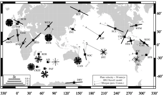
Figure 3. Map summarizing the splitting results obtained at each Geoscope station. The azimuth of the segment

represents the average fast split shear wave polarization direction φ and its length the delay time δt (reported in

Table 1). Note that the mean plotted value may be misleading for stations where several layers of anisotropy could be present (SCZ and KIP, for instance). For the stations where only null measurements were obtained, we show the backazimuthal pattern (presented in Figure 2) of the event used to help the reader to distinguish between "isotropic" stations (HYB for instance) and poorly sampled stations (AIS, for instance). Also plotted on this map are the absolute plate motion vectors at each site, the HS2-Nuvel 1 model [Gripp and Gordon, 1990] presented by the light gray arrows and data from W. J. Morgan and J. Phipps Morgan (personal communication, 1996), dark gray arrows. Note that the fast plates show a good agreement between the two models but that strong discrepancies exist for the slow moving plates (Eurasia and Africa, for instance).

of the results published in 1989 [Ansel and Nataf, 1989; Vinnik et al., 1989].

3.2 Anisotropy and Plate Motions

The lithospheric and/or asthenospheric origin of seismic anisotropy has often been debated this last decade. Observed anisotropy trends and magnitudes have been compared to the expected anisotropy related to present-day asthenospheric flow and to the surface expression of lithospheric structures. The parallelism between fast split shear waves and the trend of lithospheric structures (such as mountain belts) has led several authors to propose that the whole lithosphere could be pervasively structured during orogenies [Silver and Chan, 1988; Vauchez and Nicolas, 1991; Nicolas, 1993; Vauchez et al., 1997], freezing a noticeable part of anisotropy for long periods [Helffrich et al. , 1994; Barruol et al., 1997a]. Alternatively, the correlation between the anisotropy and the absolute plate motion (APM) observed at some stations led to a proposal that the main source of splitting could be the sublithospheric mantle, affected by a present-day flow induced by the plate motion [Vinnik et al., 1992]. The accuracy of APM directions is fundamental in this discussion. In order to test the hypothesis of anisotropy controlled by plate motion we determined at each station the APM vector calculated from two different models: HS2-Nuvel 1 by Gripp and Gordon [1990] and a model proposed by W. J. Morgan and J. Phipps Morgan (personal communication, 1996). These vectors are plotted in Figure 3 together with the splitting results. The angular differences between the observed anisotropies and the APM vectors are shown in Figure 4. Figure 4 clearly shows that no systematic correlation is present between our results and the HS2-Nuvel 1 model; only two stations display an angular difference of less than 20° between the two directions. Morgan's

APM is characterized by a better correlation with φ since half of

the 16 stations display an obliquity of <20°, suggesting that asthenospheric flow beneath the plate could explain part of the results but that it cannot be a universal explanation. These examples mainly point out that the correlation of plate motion vectors and seismic anisotropy and the subsequent interpretations largely depend on the APM data used.

As shown for the oceanic plates by Tommasi et al. [1996], a drag-induced anisotropy model should generate a positive

correlation between the plate velocity and the observed δt. Figure

4 shows that there is no direct correlation between plate velocities and the magnitudes of the delay times for both APM models; the

fastest plates do not generate the highest δt which are rather

observed on the slowest plates. In summary, the rather poor correlation between the plate motion vectors and the anisotropy parameters beneath the Geoscope stations does not favor any simple explanation such as a single anisotropic layer in the asthenosphere generated by the plate motion.

3.3 One or Two Layers of Anisotropy?

An important aim of this paper is to accurately quantify the anisotropy beneath permanent stations in order to render possible station-side anisotropy correction. On a practical point of view, a single anisotropic layer is required to perform reliable correction. The presence of dipping anisotropy or several layers of anisotropy would impede any consistent station-side anisotropy correction. Under the assumption that anisotropy is located within a single horizontal layer with a horizontal symmetry axis, little

variation of the splitting parameters (φ, δt) are expected as a

function of the event backazimuths. Silver and Savage [1994] have shown that shear wave splitting measurements in case of two layers are still valid but that the apparent anisotropy

parameters should vary with a π/2 periodicity of the backazimuth

of the incoming wave. In order to test the presence of two anisotropic layers beneath the stations, we try to detect possible backazimuthal dependence of the splitting parameters.

Angle (°) Angle (°) 0 1 2 3 4 5 -80 -60 -40 -20 0 20 40 60 80 -80 -60 -40 -20 0 20 40 60 80 φ-morgan's apm (-90/90) Count 0 1 2 3 4 Count 0 20 40 60 80 100 120 0 0.5 1 1.5 2 velocity_Morgan (mm/yr) velocity_HS2Nuvel1(mm/yr)

Plate velocity (mm/yr)

δ t (s) φ-HS2's apm (-90/90)

a

b

c

Figure 4: Histograms of difference between the observed

azimuth φ of the fast split shear waves and the trend of the

absolute plate motion (APM) (a) with the HS2-Nuvel 1 model [Gripp and Gordon, 1990] and (b) with the W. J. Morgan's (personal communication, 1996) model. These diagrams show that the APM control on the anisotropy depends strongly on the model used. (c) The observed delay times as a function of the plate velocities. No correlation is visible for both velocity

models; the largest δt are found on the slowest plates and the

fastest plates do not show the highest δt, suggesting that the

main source of anisotropy is not a present-day asthenospheric flow induced by the plate motion.

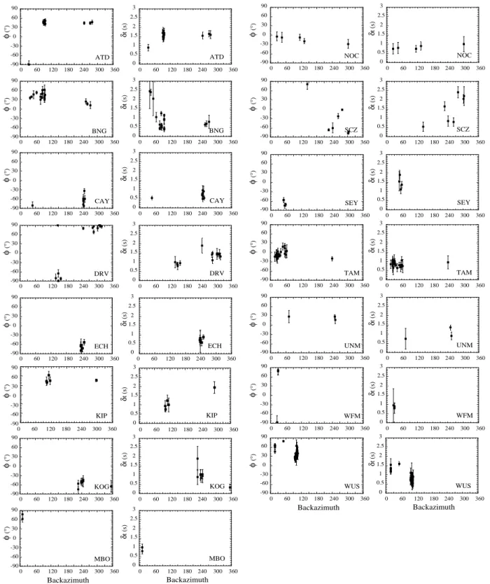
with good enough backazimuthal coverage. Figure 5 displays the

apparent φ and δt obtained at the Geoscope stations versus the

event backazimuth. Only stations characterized by more than two good nonnull measurements are shown and only good nonnull measurements are plotted together with their error bars (Table A2). At a few stations the anisotropy parameters do not show a backazimuthal dependence. This could indicate a simple structure of a single anisotropic layer but could also be due to the small number of observations (MBO, UNM, WFM) and/or to the poor backazimuthal coverage (ATD, ECH, KOG, SEY). We selected the four continental stations (DRV, SCZ, TAM, and WUS) characterized by a sufficiently large number of observations and by a good enough backazimuthal coverage to test models of two anisotropic layers. Among these four continental stations, SCZ show the strongest variations of the anisotropy parameters with the backazimuth. The three other stations display slight but

coherent variations ofφ and δt that could result from several

layers of anisotropy. The possible presence of two layers of anisotropy at KIP is discussed in the section 3.4.

Following the approach used by Savage and Silver [1993] and Silver and Savage [1994], we performed direct modeling of two horizontally layered structures and compared the predicted backazimuthal variations of the anisotropy parameters to our observations. Assuming that anisotropy in the bottom layer is related to the asthenospheric flow induced by the drag of the

plate, we fixed the fast polarization direction in this layer (φ1)

parallel to the absolute plate motion, as defined by W. J. Morgan and J. Phipps Morgan (personal communication, 1996). Anisotropy in the top layer is supposed to be related to a frozen

lithospheric deformation. The δt were fixed a priori in the lower

(δt1) and upper layer (δt2), but several values were tested, generally ranging from 0.4 to 1.2 s. For each model we calculated

the apparent φ and δt variations (φ app and δtapp) as a function of

the event backazimuth for the whole range of possible

lithospheric anisotropy directions (φ2), from N90°W to N90°E. A

few models that fit well our splitting data are shown in Figure 6. In most cases the fit between observations and theoretical curves is rather poor. This may be explained by either a strong data scattering and/or more complex structures beneath the stations than those modeled. Particularly, lateral heterogeneity in the upper mantle may combine its effects with the presence of several anisotropic layers and the crust's own structure. Nevertheless, a station by station analysis may allow one to test ideas on the magnitude and orientation of the anisotropy in the underlying mantle.

Anisotropy parameters at station TAM in the Hoggar Massif

show a slight backazimuthal dependence of φ [Ben Ismail and

Barruol, 1997]. Fixing a lower anisotropy trending N40°E, i.e. parallel to the absolute plate motion, our observations could be explained by an upper layer of anisotropy trending roughly N-S, in the range N10°E to N10°W (Figure 6). Several simple tests

with different δt suggest that the upper and lower δt could be of

the same order of magnitude. From a geological point of view this two-layer structure could be coherent with an asthenosphere deformed by the plate motion and a N-S trending structure frozen in the lithosphere. The upper lithospheric anisotropy beneath TAM is consistent with the presence of a large-scale N-S corridor of strike-slip deformation, composed of numerous strike-slip shear zones (see Figure 7), several thousand kilometers long and several hundreds of km wide [see, e.g., Boullier, 1986; Black et al., 1994; Haddoum et al., 1994]. This N-S trending anisotropy

generated the Hoggar volcanism and uplift, the N-S pervasive structures may be preserved since Panafrican times within the lithosphere. This is consistent with the ideas that strike-slip deformation may be efficient to generate strong seismic anisotropy [Vauchez and Nicolas, 1991; Mainprice and Silver, 1993] and that anisotropy may be preserved for long periods within the lithosphere [Silver, 1996; Barruol et al., 1997a; Ben Ismail and Mainprice, 1998].

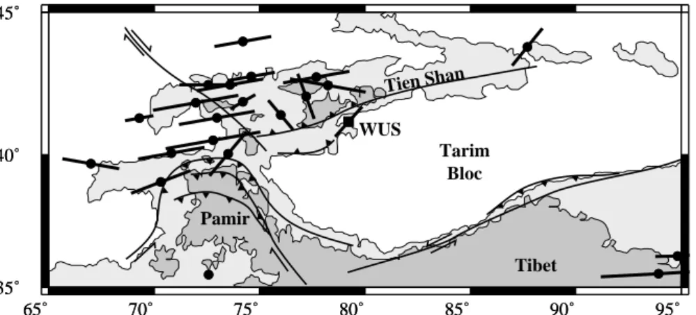
Station WUS lies on the northern boundary of the Tarim bloc, on the southern flank of the Tien Shan range (Figure 8). Although the structure is illuminated by a relatively poor backazimuthal coverage, shear wave splitting observations suggest a complex anisotropy pattern; the few events arriving at a backazimuth around N20°E display higher delay times (in the range of 1.2 to

1.6 s) than the main group arriving around N100°E (δt in the

range of 0.4 to 1.0 s). In case of a simple, horizontal two-layered structure the apparent anisotropy parameters should vary with a

π/2 periodicity. Therefore events arriving from backazimuths of

N10-N20°E should give similar results as those arriving from N100 to N110°E. This is not the case, suggesting other factors like dipping structures (that are expected to generate variations in

the apparent φ and δt with a periodicity of π) or lateral

heterogeneity to be present. We tested two-layer models to try to

fit most of our results fixing the lower φ1 parallel to the APM at

N72°W. The calculated parameters (Figure 6) do not show a good

fit for the apparent φ direction and δt. The discrepancy is

particularly strong for events with backazimuths of N20°E and an

upper φ2 trending around N50-N60°E, i.e., parallel to the Tien

Shan belt. From waveform inversions, Farra et al. [1991]

determined a two-layer model at WUS with a lower φ1 of N60°E

and an upper φ2 of N110°E, which does not fit our observations.

According to Mattauer [1986], the rigid and cold Tarim lithospheric bloc is likely subducting beneath the Tien Shan belt. The large negative Bouguer anomaly associated with the Tien Shan also suggests that the Tarim block is bent beneath the belt [Burov et al., 1990] along the subduction trending N60°E. Dipping structures beneath the station could therefore explain

part of the complicated variations of δt as a function of the

backazimuth. The parallelism of our upper φ2 with the trend of

the belt is consistent with other SKS splitting measurements in the Tien Shan published by Makeyeva et al. [1992]. Their observations plotted in Figure 8 show a parallelism of the fast split shear waves with the trend of the belt in several parts of the belt. This may result from a strong and pervasive upper mantle flow between the two rigid and convergent Tarim and Kazakh lithospheric blocs.

Station SCZ in California lies on the San Andreas strike-slip fault system. This area is the best documented two anisotropic layer region to date [Savage and Silver, 1993; Ozalaybey and Savage, 1994; Silver and Savage, 1994; Ozalaybey and Savage, 1995]. The splitting results at most of the stations lying on the San Andreas fault are consistent with two layers of anisotropy, a lower layer with an anisotropy trending N70°-N90°E and the upper one trending N50°W to N70°W. The parallelism of the

upper φ2 with the San Andreas fault strongly suggests this

anisotropy to be connected to the fault-related lithospheric strain.

Previous interpretations of the E-W trending φ in the lower

anisotropic layer favor an eastward asthenospheric flow left behind the Farallon plate [Savage and Silver, 1993; Ozalaybey and Savage, 1995]. From several tests that we made, the best fit

φ ( ° ) φ ( ° ) φ ( ° ) φ ( ° ) φ ( ° ) φ ( ° ) φ ( ° ) φ ( ° ) δ t (s) δ t (s) δ t (s) δ t (s) δ t (s) δ t (s) δ t (s) δ t (s) φ ( ° ) φ ( ° ) φ ( ° ) φ ( ° ) φ ( ° ) φ ( ° ) φ ( ° ) δ t (s) δ t (s) δ t (s) δ t (s) δ t (s) δ t (s) δ t (s) Backazimuth Backazimuth Backazimuth Backazimuth 0 60 120 180 240 300 360 0 60 120 180 240 300 360 0 60 120 180 240 300 360 0 60 120 180 240 300 360 0 0 60 120 180 240 300 360 0 60 120 180 240 300 360 0 0 60 120 180 240 300 360 0 60 120 180 240 300 360 0 60 120 180 240 300 360 0 60 120 180 240 300 360 0 60 120 180 240 300 360 0 60 120 180 240 300 360 0 60 120 180 240 300 360 0 60 120 180 240 300 360 0 60 120 180 240 300 360 0 60 120 180 240 300 360 60 120 180 240 300 360 0 60 120 180 240 300 360 0 60 120 180 240 300 360 0 60 120 180 240 300 360 0 60 120 180 240 300 360 0 60 120 180 240 300 360 0 60 120 180 240 300 360 0 60 120 180 240 300 360 0 60 120 180 240 300 360 0 60 120 180 240 300 360 60 120 180 240 300 360 0 60 120 180 240 300 360 0 60 120 180 240 300 360 0 60 120 180 240 300 360 -90 -60 -30 0 30 60 90 -90 -60 -30 0 30 60 90 -90 -60 -30 0 30 60 90 -90 -60 -30 0 30 60 90 -90 -60 -30 0 30 60 90 -90 -60 -30 0 30 60 90 -90 -60 -30 0 30 60 90 -90 -60 -30 0 30 60 0 0.5 1 1.5 2 2.5 3 0 0.5 1 1.5 2 2.5 3 0 0.5 1 1.5 2 2.5 3 0 0.5 1 1.5 2 2.5 3 0 0.5 1 1.5 2 2.5 3 0 0.5 1 1.5 2 2.5 3 0 0.5 1 1.5 2 2.5 3 0 0.5 1 1.5 2 2.5 -90 -60 -30 0 30 60 90 -90 -60 -30 0 30 60 90 -90 -60 -30 0 30 60 90 -90 -60 -30 0 30 60 90 -90 -60 -30 0 30 60 90 -90 -60 -30 0 30 60 90 -90 -60 -30 0 30 60 0 0.5 1 1.5 2 2.5 3 0 0.5 1 1.5 2 2.5 3 0 0.5 1 1.5 2 2.5 3 0 0.5 1 1.5 2 2.5 3 0 0.5 1 1.5 2 2.5 3 0 0.5 1 1.5 2 2.5 3 0 0.5 1 1.5 2 2.5 WUS WUS WFM WFM UNM UNM TAM TAM SEY SEY SCZ SCZ NOC NOC MBO MBO KOG KOG ECH ECH KIP KIP DRV DRV CAY CAY BNG BNG ATD ATD

Figure 5. High quality measurements of φ and δt as a function of the backazimuth of the events performed at the Geoscope stations. Only stations having two or more good nonnull measurements are shown and only the good results (as evaluated Table A2) are plotted. These diagrams show that the anisotropy parameters at some stations depend on the azimuth of the incoming waves. Note the rather poor backazimuthal coverage obtained at most of the Geoscope stations and the relatively small number of well-constrained teleseismic shear wave splitting measurements obtained at permanent stations.

TAM: φ1=N40°E, δt1=0.6 s ; δt2=0.6 s TAM: φ1=N40°E, δt1=0.6 s ; δt2=0.6 s

WUS : φ1=N72°W, δt1 = 0.5 s ; δt2=0.7 s WUS : φ1=N72°W, δt1 = 0.5 s ; δt2=0.7 s

SCZ : φ1= N70°E, δt1 = 1.0 s ; δt2=1.0 s SCZ : φ1= N70°E, δt1 = 1.0 s ; δt2=1.0 s

DRV : φ1= N72°E, δt1 = 0.5 s ; δt2 = 0.8 s DRV : φ1= N72°E, δt1 = 0.5 s ; δt2 = 0.8 s

POLARIZATION DIRECTION POLARIZATION DIRECTION

KIP: φ1=N58°W, δt1 = 1.0 s ; δt2=1.0 s KIP: φ1=N58°W, δt1 = 1.0 s ; δt2=1.0 s 180 210 240 270 300 330 360 180 210 240 270 300 330 360 0 60 120 180 240 300 360 0 60 120 180 240 300 360 0 30 60 90 120 150 180 0 30 60 90 120 150 180 0 30 60 90 120 150 180 0 30 60 90 120 150 180 0 60 120 180 240 300 360 0 60 120 180 240 300 360 -80 -60 -40 -20 0 0.5 1 1.5 2 2.5 3 -90 -60 -30 0 30 60 90 0 0.5 1 1.5 2 2.5 3 -40 -20 0 20 40 60 80 0 0.5 1 1.5 2 2.5 3 0 0.5 1 1.5 2 2.5 3 -100 -80 -60 -40 -20 0 20 40 0 0.5 1 1.5 2 2.5 3 0 20 40 60 80 δ t _φ δ t _φ δ t _φ δ t _φ δ t _φ δtapp (φ2=-20.) δtapp (φ2=-10.) δtapp (φ2= 0.) δtapp (φ2= 10.) δtapp (φ2= 20.) φapp (φ2=-20.) φapp (φ2=-10.) φapp (φ2= 0.) φapp (φ2= 10.) φapp (φ2= 20.) φapp (φ2= 30.) φapp (φ2= 40.) φapp (φ2= 50.) φapp (φ2= 60.) φapp (φ2=-70.) φapp (φ2=-60.) φapp (φ2=-50.) φapp (φ2=-40.) δtapp (φ2=-70.) δtapp (φ2=-60.) δtapp (φ2=-50.) δtapp (φ2=-40.) φapp (φ2=-90.) φapp (φ2=-80.) φapp (φ2=-70.) φapp (φ2= 70.) φapp (φ2= 80.) δtapp (φ2=-90.) δtapp (φ2=-80.) δtapp (φ2=-70.) δtapp (φ2= 70.) δtapp (φ2= 80.) δtapp (φ2= 50.) δtapp (φ2= 60.) δtapp (φ2= 70.) δtapp (φ2= 80.) δtapp (φ2= 90.) φapp (φ2= 50.) φapp (φ2= 60.) φapp (φ2= 70.) φapp (φ2= 80.) φapp (φ2= 90.) δtapp (φ2= 30.) δtapp (φ2= 40.) δtapp (φ2= 50.) δtapp (φ2= 60.)

lower layer trending N70°E, and a φ1 trending N50°-60°W in the

upper layer (Figure 6). Models with a lower φ1 trending parallel

to the Pacific APM (N57°W, deduced from the HS2-Nuvel 1 model) do not fit the observations. Our models therefore suggest that the anisotropy in the bottom and top layers trend parallel to the North American APM and to the strike of the San Andreas fault system, respectively. Our preferred interpretation is that two types of deformation are present beneath this zone: a pervasive upper mantle deformation with a vertical foliation parallel to the San Andreas fault and an asthenospheric deformation that could be induced by the westward motion of the whole system.

Anisotropy at station DRV, Antarctica, is characterized by small azimuthal dependence of the anisotropy parameters, with

smaller δt for waves arriving from azimuths of N150°E than from

azimuths of N50°W. A model of two layers of anisotropy may explain these slight variations (Figure 6). The best fitting model

is characterized by smaller δt in the asthenosphere (around 0.5 s)

than in the lithosphere (0.8 s) and φ1 trending around N70°E in

the lower layer and roughly E-W in the upper one. The scarce knowledge of the crustal structure in this area renders any interpretation highly speculative.

In summary, although the number of reliable data and the

backazimuthal coverage are the limiting factors in looking for several anisotropic layers, systematic investigations of S K S splitting at permanent stations may allow detection of some complex structures and the test of existing ideas. If one except station CAN where two anisotropic layers may exist with

perpendicular φ and similar δt (see discussion below), station

SCZ appears to be the only Geoscope station clearly underlain by two layers of anisotropy. The detailed analysis of the backazimuthal variations of the anisotropy parameters, as suggested by Savage and Silver [1993] allow a discussion of potential structures to explain some observations.

3.4 Anisotropy Beneath Ocean Island Stations

Six stations of the Geoscope network lie on ocean islands; two in the Pacific (KIP and PPT) and four in the Indian Ocean (RER, PAF, AIS and CRZF). Data recorded on oceanic islands are of low quality because of the high level of background noise (sea waves). Regarding our results with respect to the geological particularity of ocean island, our results are worth a short discussion.

At the Indian Ocean stations (Figure 9) we were not able to characterize any clear anisotropic structure. At PAF, a single nonnull measurement was obtained but of only fair quality and therefore cannot be considered as reliable. At RER, two nonnulls were recorded (see Table A2) but none of good quality. At CRZF, numerous null measurements of good quality with a good backazimuthal coverage argue for an apparent isotropy for the S waves along the vertical direction. At AIS the small number of measurements due to only 3 years of available data but also to strong background noise in the seismograms did not allow an accurate anisotropy characterization.

The apparent isotropy deduced from SKS splitting at these stations may either be related to the internal structure of the lithosphere and asthenosphere or to the local hot spot activity under the stations that could have erased the pervasive structure of the lithosphere or at least affected the structure enough to render anisotropy difficult to detect. Lévêque et al. [1998] inferred a disturbing effect induced by the hot spot at La Réunion: The good correlation between the fast anisotropic direction and the APM between 100 and 200 km depth present on most of the plate is lost in this particular region. Since a large-scale anisotropy pattern is observed beneath the whole Indian Ocean down to 300 km depth from surface waves [Lévêque et al., 1998], we also suggest that the apparent isotropy deduced from SKS splitting may be primarily related to the complex structures beneath the volcanic island stations induced by hot spot activity.

In the Pacific ocean, PPT appears to be isotropic. This result is not supported by a large number of measurements (see Table A2 and Figure 2) but is consistent with that of Russo and Okal [1998]

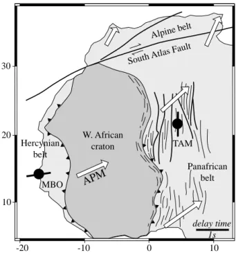
Figure 7. Seismic anisotropy on the west African continent.

Our observations made at MBO and TAM are presented, together with a schematic tectonic map and the APM vectors calculated from W. J. Morgan's (personal communication, 1996) model. Anisotropy at TAM displays a clear parallelism with the N-S trending Panafrican strike-slip zones and a poor correlation to the present-day motion of the African plate.

Figure 6. Apparent variations in the observed anisotropy parameters with a π/2 periodicity may be related to the presence of two anisotropic layers beneath the station. We calculated simple models of two anisotropic layers that could explain

apparent variations in the anisotropy parameters φ and δt that we observed at well characterized stations. For each station

we plot the apparent variations of the observed delay time (δtapp, left) and azimuth of the fast split shear wave (φapp, right)

as a function of the backazimuth of the incoming wave. The curves represent the predicted variations of the apparent φ and

δt in case of two anisotropic layers together with our observations and the corresponding error bars. In the models the

anisotropy parameters of the lower layer are fixed (φ1 and δt1), together with the upper layer delay time (δt2); φ1 is chosen

parallel to the absolute plate motion. The different curves correspond to possible anisotropy trends (φ2) in the upper layer

that best fit our observations and which could reflect a lithospheric anisotropy. 20 30 10 -10 -20 0 10 South Atl as Fault Alpine be lt delay time 1s Panafrican belt W. African craton TAM MBO Hercynian belt

APM

Figure 8. Seismic anisotropy in the Tien Shan. Together with our mean result obtained at the Geoscope station WUS,

we show the anisotropy results obtained by Makeyeva et al. [1992] and the main faults. The two gray levels represent the 2000 and 4000 m topography.

Figure 9. Location of the four Geoscope stations in the Indian Ocean, where we failed to detect anisotropy. The

isochrons of the age of the oceanic plate are superimposed to the plate topography (ETOPO5). Together with the null observations, the HS2-Nuvel 1's APM [Gripp and Gordon, 1990] is represented by the dark arrows and W. J. Morgan's (personal communication, 1996) APM by the light gray arrows.

Tarim Bloc Pamir Tibet WUS Tien Shan 65˚ 70˚ 75˚ 80˚ 85˚ 90˚ 95˚ 35˚ 40˚ 65˚ 70˚ 75˚ 80˚ 85˚ 90˚ 95˚ 35˚ 40˚

20˚

30˚

40˚

50˚

60˚

70˚

80˚

90˚

100˚

-60˚

-50˚

-40˚

-30˚

-20˚

-10˚

0˚

20˚

30˚

40˚

50˚

60˚

70˚

80˚

90˚

100˚

-60˚

-50˚

-40˚

-30˚

-20˚

-10˚

0˚

RER

AIS

PAF

CRZF

Plate velocity = 9 mm/yr HS2-Nuvel1 model Morgan (pers. Com.)

and Wolfe and Silver [1998] plotted in Figure 10. At KIP, four events showed SKS splitting, two of them of good quality. Assuming a single anisotropic layer, the mean splitting

parameters we found are φ = N45°E and δt = 1.1 s. None of the

expected structures under the Oahu island (present-day APM, former APM, expansion direction, orientation of the transforms) alone may explain this trend of a

nisotropy, suggesting the presence of several layers of anisotropy or a different source of anisotropy.

The Pacific plate at both stations, KIP and PPT, is moving fast (around 8 cm/yr). Absolute velocities and directions are well constrained by numerous hot spot related island chains. The Emperor chain suggests a major change in the APM about 43 Ma from N-10°E to N58°W. Assuming that the lithosphere thickens with age and freezes asthenospheric material at its base, a change in the plate motion should result in a change of olivine fabric orientation with depth [Tommasi, 1998]. The upper layer should be characterized by a fast polarization direction close to the fossil Pacific plate motion direction and the lower layer anisotropy should be controlled by the present-day plate motion vector.

Following the scheme described in section 3.3, we fixed φ1 in the

bottom layer to the present-day APM direction (N58°W) and

tested different φ2 directions in the upper layer and various delay

times for both layers. The model characterized by anisotropies in

the bottom and top layer related to the present-day and former APM, respectively, does not fit the observations. Although the

data sets are different, the best models shown Figure 6 (φ1 =

N58°W, δt1 = 1.0 s, φ2 = N80°E, δt2 = 1.0 s) give values

comparable to those of Wolfe and Silver [1998] in direction but

with slightly larger δt (φ1 = N58°W, δt1 = 0.45 s, φ2 = N75°E,

δt2 = 0.75 s). The upper anisotropy is not parallel to the paleo-APM but seems to be oriented close to the trend of the transform zone (the Molokai fracture zone) underneath the Oahu island (see Figure 10). This parallelism may have various explanations: (1) The present-day anisotropy of this fracture zone in the lithosphere is not dominated by olivine lattice preferred orientation but by other pervasive structures such as microfracturation or vertical layering. (2) The frozen olivine fabric within the lithosphere before 43 Ma was induced by the fracture zone itself. (3) The asthenospheric flow before 43 Ma was affected by the lithospheric step related to the fracture zone that separated domains of different ages and therefore of different lithospheric thickness [Tommasi et al., 1996].

3.5 Upper Mantle Isotropy?

Three continental Geoscope stations (CAN, HYB, and SSB) are characterized by an apparent absence of detectable

180˚

190˚

200˚

210˚

220˚

230˚

240˚

-30˚

-20˚

-10˚

0˚

10˚

20˚

30˚

180˚

190˚

200˚

210˚

220˚

230˚

240˚

-30˚

-20˚

-10˚

0˚

10˚

20˚

30˚

KIP

TPT

PPT

TBI

RAR

AFI

PS

Plate velocity = 100 mm/yr HS2-Nuvel1 model

Figure 10. Seismic anisotropy in the Pacific. Together with the plate isochrons and plate topography, the APM

vector (HS2-Nuvel 1) and our null results at PPT, are shown the anisotropy measurements from Russo and Okal [1998] at the stations TPT and TBI, from Silver and Wolfe [1998] at RAR and AFI, the PS bounce phase splitting done by Su and Park [1994], and our mean result at KIP. Close to KIP, we also plot the two anisotropic directions that could explain the backazimuthal anisotropy variations observed: an upper anisotropy parallel to the expansion direction (solid line) and a lower anisotropy parallel to the present-day APM (dashed line).

respectively) and are well documented by numerous null measurements of good quality and very few nonnull measurements of lower quality (see corresponding patterns Figures 2 and 3).

Splitting measurements at CAN, eastern Australia, have given 48 nulls (from which 18 are of good quality) with a rather good backazimuthal coverage (see Figure 3) and only four nonnull splitting measurements. From these four nonnulls, a single one seems to be of good quality: event 93010 (Table A2) from which

we obtained φ = N66°E and δt = 0.90 s. However, the SKS and S

phases are close from each other (the distance of this event is only 86°), and part of the results could reflect the S phase splitting. It is interesting to note that the apparent isotropy that we observed at CAN is consistent with other recent observations in Australia [Clitheroe and van der Hilst, 1998; Girardin and Farra, 1998] that show complex upper mantle structures.

At HYB, India, 96 null measurements (53 of which are of good quality) and only five nonnull events were found, two of them deduced from deep event S phases. None of these five measurements is of good enough quality to be reliable. Figures 2 and 3 clearly show the good backazimuthal coverage of this station documenting particularly well this apparent absence of anisotropy.

At SSB we measured about 70 nulls (see Table A2) with a good backazimuthal coverage (see Figure 2), 35 of them of good quality, and eight non null splitting measurements. Among the latter, owing to the small energy on the transverse component, two are close to nulls (events 90290 and 94231) and appear as weakly reliable. Only two events (93284 and 96255) gave good splitting measurements (see Table A2). Both come from very similar backazimuths (N38°E and N34°E, respectively) and give

very similar anisotropy parameters (φ = N145°E, δt = 0.80 s

and φ = N157°E, δt = 0.50 s, respectively). These results are

consistent with the nulls oriented around N60°E observed by Ansel and Nataf [1989] and with the non null result obtained by Vinnik et al. [1989] (φ = N140°E and δt = 1.0 s).

The absence of teleseismic shear wave splitting for a large range of backazimuths is quite uncommon (see list of stations from Silver [1996]). Such isotropy has been observed for instance in the Rocky Mountains [Savage et al., 1996], in the Pakistan Himalaya [Sandvol et al., 1994] or at some stations in the eastern United States [Barruol et al., 1997b]) and rarely documented by as many null measurements as presented here; it may result from several structures and processes :

1. The absence of shear wave splitting may simply result from the absence of anisotropy beneath the station. This interpretation implies that the whole upper mantle displays no large-scale pervasive structure, i.e., that both the lithosphere and asthenosphere are isotropic. Observations of natural samples of lithospheric mantle rocks do not favor this hypothesis. Rocks taken from peridotite massifs or from xenoliths brought up to the surface by kimberlitic or basaltic volcanism systematically show olivine lattice preferred orientation, clearly distinguishable from reworking related to extraction or emplacement processes [Boullier and Nicolas, 1975; Mercier and Nicolas, 1975; Boudier et al., 1984; Mainprice and Silver, 1993; Ji et al., 1994; Barruol and Kern, 1996; Kern et al., 1996]. Since anisotropy appears to be an ubiquitous upper mantle property, this case should be exceptional.

2. The absence of shear wave splitting may result from heterogeneities. The anisotropy is a function of the scale of observation and of the wavelength of the shear phases [see

scale, for instance) the medium may be anisotropic, but large variations in the structure orientation may render it isotropic at a larger scale. In particular, the presence of numerous anisotropic layers with random fast axis orientations could average the medium property to an apparent isotropy.

3. The absence of shear wave splitting may result from vertically oriented lineations in the mantle beneath the station. Petrophysical analyses of peridotites [e.g., Mainprice and Silver, 1993; Ji et al., 1994; Kern et al., 1996; Mainprice et al., 1997; Ben Ismail and Mainprice, 1998] show that the X structural axis, i.e., the rock lineation marked by the olivine a axis concentration, is generally characterized by a weak anisotropy. The absence of anisotropy observed at some rift stations [Gao et al., 1997] or on the Colorado plateau [Savage et al., 1996; Sheehan et al., 1997] could be explained by vertical asthenospheric upwelling inducing vertical lineations in the upper mantle. The isotropy beneath the French Massif Central station SSB could also result from such a structure; asthenospheric diapirism indeed has been described beneath the Massif Central [Nicolas et al., 1987] and the lithospheric thickness determined by seismic tomography [Granet et al., 1995] or by geochemistry [Werling and Altherr, 1997] is small. The few nonnull splitting measurements obtained at this station by events arriving from backazimuths around N30°E may suggest lateral heterogeneities.

4. The absence of apparent shear wave splitting may result from the presence of two anisotropic layers, characterized by perpendicular fast axes azimuths and by similar delay times in each layer. In such a particular structure, the top layer should physically remove the splitting acquired in the bottom layer. The apparent isotropy observed at HYB and CAN is particularly surprising because of the relative fast absolute plate motion (oriented close to N-S and around 5 and 7 cm/yr, respectively) that should generate detectable asthenospheric anisotropy, assuming the lithosphere homogeneously moves on the flowing asthenosphere. The deep lithospheric structures beneath these sites are poorly known. A roughly E-W trending lithospheric frozen anisotropy superimposed on a roughly N-S asthenospheric anisotropy could explain the absence of SKS splitting observed at this station. Interestingly, such a model is independently suggested for station CAN by Girardin and Farra [1998] from different observations. From P-to-S converted waves at upper mantle interfaces, they infer that two layers of anisotropy may

exist beneath this site, the upper one with an E-W trending φ and

the lower one with a N-S trending φ.

3.6 Anisotropy at Some Geologic Structures

In the sections 3.1-3.5, seismic anisotropy measurements have been discussed for many stations taking into account their geodynamic situation, particularly for the stations that could lie above two anisotropic layers, for the oceanic stations and for the "isotropic" continental stations. The results obtained at several other stations (ATD, ECH, NOC, and SEY) located on interesting geologic structures and characterized by consistent results will be discussed in the following. A discussion on anisotropy at WFM in the eastern United States may be found in a previous study [Barruol et al., 1997b].

Seismic anisotropy at ATD, Djibouti, is one of the largest and best constrained in the Geoscope network. This station lies on the African side of the Afar triple junction, between the Red Sea rift,

the east African rift, and the Gulf of Aden. The anisotropy (φ =

the East African Rift. This result is consistent with measurements made by Gao et al. [1997] and by Ben Ismail and Barruol [1997] on the Kenya rift farther south. Both studies found fast split shear waves oriented parallel to the rift trend and rather high delay times for the stations lying on the rift itself. Such a striking parallelism suggests that the anisotropy could be related to deep rift structures and the rifting processes. Since lattice preferred orientations can develop under asthenospheric conditions [Nicolas and Christensen, 1987], an asthenospheric flow channeled beneath the rift could provide an important source of anisotropy [Nicolas, 1993; Nicolas et al., 1994]. Since ATD is close to the Afar triple junction, anisotropy may also be influenced by the plume-related upper mantle flow.

The good anisotropy measurements performed at ECH, in the Vosges Massif in France seem to indicate that the anisotropy trends N110-120°E with a delay time of around 0.70 s. This anisotropy direction does not follow the Hercynian lithospheric

structures, oriented more NE-SW in this massif. Instead, φ is

roughly normal to the trend of the Rhine graben, a few tenths of a kilometers to the east, imaged by seismic tomography [Glahn et al., 1993]. Some less constrained splitting results indicate an anisotropy trending NE-SW, a direction also observed by Granet et al. [1998], suggesting a complex anisotropy pattern beneath this area. Since all the good measurements were obtained from events with similar backazimuths around N240-250°E (see Figure 5), we are not able to go into detail about more complex structures.

Anisotropy at NOC, New Caledonia, is well defined (φ =

N166°E; δt = 0.82 s). Given the absolute plate motion direction,

roughly N-S in this area, and the relatively high velocity of the Australian plate (around 7 cm/yr), the anisotropy at this station could be explained by frozen lithospheric structure and present-day asthenospheric deformation, both induced by the plate drag. However, this plate is subducting at its northern and eastern boundaries, respectively in the Java-Sumatra-New Guinea and New Hebrides trenches. This led Silver and Russo [1995] to propose that anisotropy north of Australia could be related to the closure of the oceanic domain between the thick Australian continental lithosphere [Gaherty and Jordan, 1995] and the subduction zone, both forming flow barriers. A similar model was proposed by Russo and Silver [1994] for the upper mantle flow induced by the retrograde motion of the subducting Nazca plate beneath the South American plate. Assuming that lateral expulsion of the upper mantle requires less energy than pushing the material into the upper mantle transition zone, such a process should generate trench-parallel anisotropies. The parallelism of the fast split shear wave observed at NOC with the trend of the New Hebrides trench is consistent with a southward expulsion of upper mantle material along the slab. Measurements of upper mantle anisotropy at a station in northern Australia on deep events from the Indonesian and New Guinea trenches [Tong et al., 1994] may also support this interpretation.

Anisotropy at SEY, northeastern Russia, is also rather well

defined (φ = N116°E, δt = 1.43 s). This station lies on the

Verkhoyansk fold belt [Zonenshain et al., 1990], which corresponds to a deformed zone of Paleozoic to Jurassic clastic series accumulated along the eastern edge of the Siberian platform. This passive margin has been accreted along the Siberian craton boundary by a collision during upper Jurassic times. The structural trend of this belt clearly wraps around the craton's edge that could have acted as a rigid lithospheric heterogeneity. In the SEY region the structures trend roughly

NW-SE and display a good parallelism with the observed φ,

suggesting that the lithospheric mantle beneath this station could be coherently affected by this collision.

4 Conclusions

Systematic investigation of SKS splitting at stations from the Geoscope global network allowed us to accurately characterize the upper mantle anisotropy beneath about half of the stations. The large number of measurements at some sites permits us to discuss the presence of several layers of anisotropy. Only one Geoscope station (SCZ in California) appears to be clearly underlain by two anisotropic layers. Upper mantle structures beneath stations lying above subduction zones (INU in Japan, HDC, ICC, and PEL in south America) require future work, in particular, using direct S wave splitting, in order to characterize the various anisotropic layers, i.e., beneath, within, and above the slab.

Systematic SKS splitting measurements at the Geoscope global network do not favor any global anisotropy pattern and hence a unique and global anisotropy interpretation. This suggests that the various sources of anisotropy and that the various processes that generated them strongly depend on the geodynamic environment and on the regional tectonic history.

The lack of correlation of anisotropy parameters with absolute plate motion vectors does not permit detection of a clear asthenospheric signature of anisotropy. A few stations show a good correlation of the anisotropy orientation with the trend of lithospheric faults: At TAM the anisotropy is parallel to the N-S trending Panafrican system of strike-slip faults strongly suggesting a lithospheric origin of the signal. At SCZ the upper anisotropic layer, likely related to the present-day lithospheric deformation, trends exactly parallel to the San Andreas fault.

Except at KIP in the Pacific Ocean, we failed to observe seismic anisotropy in the ocean basins. In the Indian Ocean, mainly nulls were observed. The situation of these stations on hot spot related volcanic islands may indicate that the upper mantle beneath these sites has a complex structure likely composed of a frozen lithospheric deformation, a present-day flow in the asthenosphere related to the plate motion, and a frozen or active flow related to the fossil or active hot spot activity.

At three Geoscope stations, numerous null measurements suggest an apparent upper mantle isotropy beneath the stations for vertically propagating shear waves. We examine the various factors that may induce this absence of shear wave splitting. We propose that the isotropy at SSB in the French Massif Central could be related to a mantle upwelling and to vertically oriented olivine lineations whereas the apparent isotropy at CAN, and perhaps at HYB, could be generated by two layers of anisotropy

with perpendicular φ and roughly similar δt.

One of the aims of this paper and of the discussion was to provide a list of the Geoscope stations that may be used for anisotropy correction purposes. We sort the stations into three groups depending on their general quality. A first group of stations cannot reasonably be used for remote anisotropy search due to the presence of two anisotropic layers (SCZ), to the too small number of SKS measurements performed at these sites (CAY, HDC, INU, KOG, MBO, PEL, and UNM) or the too noisy records (for instance, at most of the ocean island stations). BNG, ECH, NOC, SEY, WFM, and WUS represent the second group of stations. They may reasonably be used for anisotropy correction but require some precautions. At these sites, anisotropy seems to be well defined, but some variations in the anisotropy parameters