HAL Id: insu-03088396
https://hal-insu.archives-ouvertes.fr/insu-03088396v2
Submitted on 7 May 2021
HAL is a multi-disciplinary open access
archive for the deposit and dissemination of
sci-entific research documents, whether they are
pub-lished or not. The documents may come from
teaching and research institutions in France or
abroad, or from public or private research centers.
L’archive ouverte pluridisciplinaire HAL, est
destinée au dépôt et à la diffusion de documents
scientifiques de niveau recherche, publiés ou non,
émanant des établissements d’enseignement et de
recherche français ou étrangers, des laboratoires
publics ou privés.
Distributed under a Creative Commons Attribution - NonCommercial| 4.0 International
ammonia derived from a decadal (2008-2018) satellite
record
Martin van Damme, Lieven Clarisse, Bruno Franco, Mark Sutton, Jan Willem
Erisman, Roy Wichink Kruit, Margreet van Zanten, Simon Whitburn, Juliette
Hadji-Lazaro, Daniel Hurtmans, et al.
To cite this version:
Martin van Damme, Lieven Clarisse, Bruno Franco, Mark Sutton, Jan Willem Erisman, et al.. Global,
regional and national trends of atmospheric ammonia derived from a decadal (2008-2018)
satel-lite record. Environmental Research Letters, IOP Publishing, 2021, 16, pp.055017.
�10.1088/1748-9326/abd5e0�. �insu-03088396v2�
Global, regional and national trends of atmospheric ammonia derived
from a decadal (2008–2018) satellite record
To cite this article: Martin Van Damme et al 2021 Environ. Res. Lett. 16 055017
View the article online for updates and enhancements.
OPEN ACCESS
RECEIVED
17 November 2020
REVISED
14 December 2020
ACCEPTED FOR PUBLICATION
22 December 2020
PUBLISHED
6 May 2021 Original Content from this work may be used under the terms of the
Creative Commons Attribution 4.0 licence. Any further distribution of this work must maintain attribution to the author(s) and the title of the work, journal citation and DOI.
LETTER
Global, regional and national trends of atmospheric ammonia
derived from a decadal (2008–2018) satellite record
Martin Van Damme1,∗, Lieven Clarisse1, Bruno Franco1, Mark A Sutton2, Jan Willem Erisman3,
Roy Wichink Kruit4, Margreet van Zanten4, Simon Whitburn1, Juliette Hadji-Lazaro5,
Daniel Hurtmans1, Cathy Clerbaux1,5and Pierre-François Coheur1
1 Université libre de Bruxelles (ULB), Spectroscopy, Quantum Chemistry and Atmospheric Remote Sensing (SQUARES), Brussels,
Belgium
2 UK Centre for Ecology and Hydrology, Edinburgh, United Kingdom
3 Institute of Environmental Sciences, Leiden University, Leiden, The Netherlands
4 National Institute for Public Health and the Environment (RIVM), Bilthoven, The Netherlands 5 LATMOS/IPSL, Sorbonne Université, UVSQ, CNRS, Paris, France
∗
Author to whom any correspondence should be addressed. E-mail:martin.van.damme@ulb.ac.be
Keywords: ammonia (NH3), trends, emission, agriculture, biomass burning, IASI, satellite
Abstract
Excess atmospheric ammonia (NH
3) leads to deleterious effects on biodiversity, ecosystems, air
quality and health, and it is therefore essential to monitor its budget and temporal evolution.
Hyperspectral infrared satellite sounders provide daily NH
3observations at global scale for over a
decade. Here we use the version 3 of the Infrared Atmospheric Sounding Interferometer (IASI)
NH
3dataset to derive global, regional and national trends from 2008 to 2018. We find a worldwide
increase of 12.8
± 1.3 % over this 11-year period, driven by large increases in east Asia
(5.80
± 0.61% increase per year), western and central Africa (2.58 ± 0.23 % yr
−1), North America
(2.40
± 0.45 % yr
−1) and western and southern Europe (1.90
± 0.43 % yr
−1). These are also seen
in the Indo-Gangetic Plain, while the southwestern part of India exhibits decreasing trends.
Reported national trends are analyzed in the light of changing anthropogenic and pyrogenic NH
3emissions, meteorological conditions and the impact of sulfur and nitrogen oxides emissions,
which alter the atmospheric lifetime of NH
3. We end with a short case study dedicated to the
Netherlands and the ‘Dutch Nitrogen crisis’ of 2019.
1. Introduction
Ammonia (NH3) is the most abundant alkaline
com-ponent of our atmosphere. Agricultural activities are responsible for the majority of its emissions [1], with volatilization from livestock manure and losses from synthetic fertilizer application accounting for over 80 % of the total emissions in, e.g. Europe [2], United States (U.S.) [3] and China [4]. For 2015, the Emission Database for Global Atmospheric Research (EDGAR) v5.0 reports a global emission total of 49.1 Tg NH3, with 85.7 % originating from
agricul-ture [5,6]. Other sources include oceans and soils, waste water treatment, wild animals, human excreta, traffic and biomass burning [1, 7]. The latter was estimated to amount to 4.9 Tg in 2015 by the Global Fire Emissions Database (GFED) v4.1 s [8]. Recently, emissions from industry have also been identified as
an important and largely underestimated source of atmospheric NH3[9].
High NH3 levels negatively affect ecosystems by
depleting biodiversity and degrading soil and water
quality [10, 11]. Atmospheric NH3 has a
remark-able short atmospheric lifetime of the order of hours [9,12]. Once emitted, a large part of NH3 is
rap-idly deposited on terrestrial and aquatic ecosys-tems, resulting in adverse acidifying and eutrophy-ing effects [13, 14]. In combination with nitrogen (NOx) and sulfur oxides (SOx), NH3 plays a
signi-ficant role in fine particulate matter (PM2.5)
forma-tion and related health impacts [15,16]. Its contribu-tion to PM2.5formation is however still underexposed
(e.g. [17–19]) and, as regulations are mostly geared towards restricting NOxand SOxemissions, the world
is currently ‘ammonia-rich’ [20]. In Europe, China and the U.S. in particular, reduction in emissions of
nitrogen and sulfur oxides have demonstrably resul-ted in an increased amount of atmospheric gas-phase NH3 during the last decade [21–24]. Several studies
have concluded that reducing NH3 emissions would
be a cost-effective strategy to reduce PM2.5
concentra-tions [17,25]. It has been estimated that a 50 %
reduc-tion of the NH3 emissions in northwestern Europe
would lead to a 24 % reduction in the PM2.5
con-centration [26]. In China, the same reduction rate
on NH3emissions, joined with a 15 % reduction on
NOxand SOxemissions, would reduce PM2.5
pollu-tion by 11 %–17 % and nitrogen deposipollu-tion by 34 %, but would worsen acid rain [27]. Through its role in aerosol formation and the impact of its deposition
on plant productivity and carbon uptake, NH3also
affects climate [28,29].
For the first decade of the 21st century, the EDGAR emissions model reports a 20 % increase
of the global NH3 emissions, but with large
vari-ations at regional and national scales [30]. Countries in Europe have committed to modest reductions of
NH3emissions in the framework of the Gothenburg
Protocol, which is part of the convention on Long-Range Transboundary Air Pollution (LRTAP) and the
National Emissions Ceilings (NEC) Directive [31].
The success of this and other ammonia-control ini-tiatives has traditionally been difficult to assess as the uncertainty in NH3emissions is the largest among all
pollutants [1,5]. For more than a decade now, satel-lite missions offer global observations of NH3
abund-ance [32–35]. In particular, satellite-based datasets have already been used to identify and quantify main NH3point sources [9,12,36], to derive first changes
in atmospheric NH3 [37, 38], to constrain
depos-ition flux estimates [39–41] and, recently, to perform inverse modeling of NH3emissions [42,43].
The present study uses the reanalyzed NH3
data-set recently obtained from the Infrared Atmospheric Sounding Interferometer (IASI) satellite over 11 years (2008–2018) to derive decadal trends throughout the world. In the next section, the satellite data are presen-ted along with the method to derive trends and associated uncertainties. In section 3, these trends are presented, discussed and interpreted at global, regional and national scales. In the last section, a spe-cial focus is given to the case of the Netherlands, a country that received a lot of attention end of 2019 due to the ‘Dutch Nitrogen crisis’ which substantially affected the national economy [44].
2. Data and methods
2.1. Satellite measurementsEven though IASI’s main goal is to provide tem-perature and humidity measurements for improved weather forecasts, its instrumental characteristics enable global bi-daily measurements of a series of atmospheric constituents. In particular, its relatively high spatial resolution (12 km at nadir), scanning
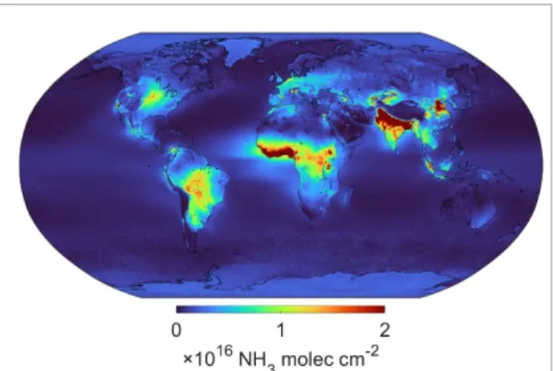
Figure 1. IASI-NH3total columns distribution
(molec cm−2) averaged from 11 years of IASI/Metop-A measurements (1 January 2008 to 31 December 2018, morning overpasses, ANNI-NH3-v3R-ERA5 dataset) on a
0.5◦× 0.5◦grid.
mode (2100 km swath) and good spectral
perform-ance (0.5 cm−1 spectral resolution apodized and
low radiometric noise) [45] have proven to be most useful for characterizing the spatiotemporal vari-ability and budget of NH3 [9, 32, 46–51]. The
IASI mission consists of a suite of three identical instruments embarked on the Metop-A, -B and -C platforms, launched in 2006, 2012 and 2018, respect-ively. Together, these provide consistent global satel-lite measurements, allowing us to derive trends at global, regional and national scale. Eleven years of morning overpass IASI/Metop-A measurements have been considered here for the calculation of the global trends, while merged IASI/Metop-A (2008–2018) and -B (2013–2018) data have been used for the case study over the Netherlands. Only morning observations have been kept as their uncertainties are lower thanks to a more favorable thermal state of the atmosphere for the remote sensing of its lowest layers [46,47].
We used version 3 of the IASI-NH3 dataset,
which was built using the ANNI (artificial neural network for IASI) retrieval framework. ANNI has been developed to perform global retrievals of NH3
[52,53] and was recently expanded to retrieve several other trace gases (e.g. [54–56]). Two IASI-NH3
data-sets are available: a near-real time dataset, for which the retrieval relies on meteorological information dir-ectly obtained from the IASI measurements [57] and a reanalyzed dataset that is based on data from the European Centre for Medium-Range Weather Fore-casts (ECMWF) climate reanalysis [58]. The latter,
named ANNI-NH3-v3R-ERA5, has been developed
specifically for trend studies and is the one used here. Its 2008–2018 globally averaged distribution is shown in figure1. Note that the satellite NH3
val-ues are reported as total columns, representing the
total number of NH3molecules in a column from the
ground surface to the top of the atmosphere expressed per unit of surface.
The general NH3 retrieval algorithm is detailed
implemented for version 3 is provided in appendixA. A careful analysis of the initial dataset revealed some spurious trends and offsets in the long-term trends over remote oceans. These included (a) two offsets that coincide with changes to the instrument, (b) a slow decreasing trend most likely due to increasing CO2concentrations and (c) a residual dependence on
H2O. Therefore, for the final version of the product,
several debiasing procedures were applied (see again appendixA). The only potential remaining source of temporal inhomogeneity stems from the use of the IASI near real-time cloud detection algorithm, as cur-rently no official reanalyzed cloud product is avail-able. This most notably affects observations over the Southern Ocean and South Pacific Ocean before 2011
[59]. IASI-NH3 measurements have been compared
with ground-based and airborne independent obser-vations in [60,61]. More recently, a dedicated valida-tion study was performed for version 3 of the product. A good correlation was found between in-situ ver-tical profiles and IASI-NH3total columns for both v3
datasets, with slightly better statistics for the reana-lysis than for the near-real time product [62]. 2.2. Trend analysis method, figures and tables
To determine the NH3 trends and their uncertainty,
the method developed by Gardiner et al [63] has
been applied to the IASI observational time series. It relies on least squares regression and bootstrap res-ampling [64] to fit daily time series data to the fol-lowing function: NH3(t) = ct + 3 ∑ n=0 [ansin(2πnt) + bncos(2πnt)]. (1)
The first term in this equation characterizes the long-term linear trend in the data, with the sought-after annual trend c. The other terms constitute a third-order Fourier series representing the periodic seasonal variations. This statistical method provides separate 2σ (or p = 0.05) lower and upper bound uncertainties of the trend values, but as the differences between both are very small, we used similarly to [63] the mean uncertainty. Following the nomenclature of that paper too, we call trends ‘significant’ if the change in NH3total columns exceeds their uncertainty (i.e. is
significantly different from zero). Trends were com-puted at grid cell, country, regional and global scales in absolute (in molec cm−2yr−1) terms. From these, we calculated total relative changes from 2008 to 2018 (i.e. the relative decadal NH3changes with respect to
2008, in % 10yr−1) and average yearly relative trends
assuming compound change rates (in % yr−1). All
uncertainties on the trend numbers, relative or abso-lute, have been reported with two significant figures.
The global distribution of the NH3 trends at
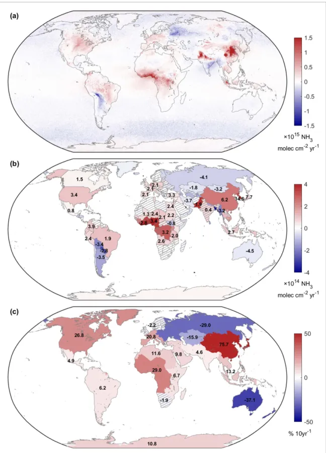
0.5◦ × 0.5◦ resolution (56 km × 56 km at the equator) is shown in figure2(a) in absolute value. Here the trend calculation was applied on each grid
cell separately. The same figure is shown (figureB1) but with stippled cells for non-significant trends. The
national trends presented in tables 1 and B1 and
in figure 2(b) were computed based on the daily
average time series at the national scale. Examples
of such daily time series are given in appendix B,
figureB3. These figures also show separately the linear and periodic terms of the fit, together with a stand-ard ordinary least squares regression fit. Trends cal-culated with the latter were generally found to be in good agreement with the trends calculated with the more robust bootstrapping method. For
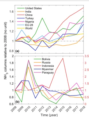
selec-ted countries we show in figure3yearly normalized
NH3 time series which were calculated from daily
averages. Global and subcontinental trends (table1, figures2(c) and B2) have been calculated based on the national numbers, weighted by the area of each country. In figures2(b) and (c), countries or subcon-tinents with non-significant trends in atmospheric
NH3 have been hatched. These thus correspond to
regions where either the uncertainty on the trend is too large or where the estimated trend is close to zero. Apart from IASI-derived trends, we also obtained trends based on yearly emission from the aforemen-tioned EDGAR bottom-up emission inventory (for 2008–2015) and the GFED inventory for pyrogenic
NH3 emission (2008–2018). These were calculated
using a standard least squares linear regression fit and are shown in appendixB, figuresB4andB5.
3. Global, regional and national trends
East Asia stands out as the region in the world with the largest increase over 2008–2018 with a decadal
increase of 75.7 ± 6.3 % and an annual growth
rate of 5.80± 0.61 % yr−1, mostly due to increases observed in the North China Plain and the Chengdu
(Sichuan, China) area (figures 2(a) and B1). For
China as a whole, we estimate an annual trend of 6.25± 0.68 % (figure 2(b)) and a decadal change
of 83.3± 7.0 %. The increased columns are likely
driven by a rise in emissions, which [4] and [65]
estimated to be 1.9 and 1.7 % yr−1 over 2000–2015
and 2008–2016, respectively. While agriculture still contributes to over 80 % of the emissions, recent emission-based [65] and satellite-based [9] studies have pointed out the increasing importance of non-agricultural sources, especially of industrial emitters. The contribution of fossil-fuel combustion sources, including traffic, has been lately highlighted espe-cially during severe haze episodes [66–68]. Surpris-ingly, as shown in figureB4, the EDGAR v5.0 global
database [6] reports a moderately slow decline in
emissions over eastern China during the 2008–2015 period, which appears to be mostly due to a sharp decline in the estimates of the year 2014 and which is not observed in the satellite data. Other studies also reported relative stable emissions during the past dec-ade (e.g. [69]).
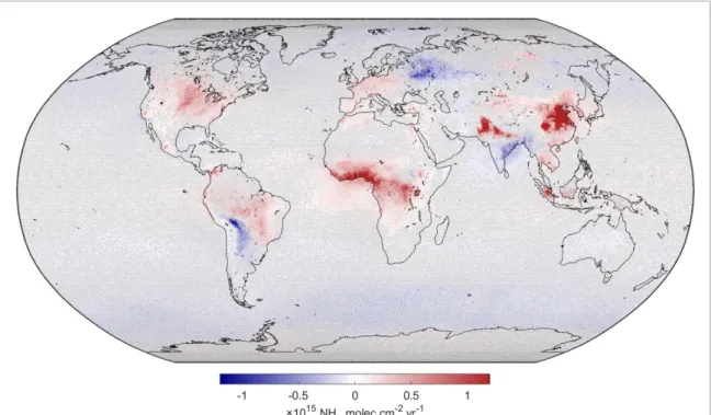
Figure 2. NH3trends based on IASI daily time series (2008–2018) for each 0.5◦× 0.5◦cell (a, molec cm−2yr−1), at the national
(b, molec cm−2yr−1) and regional (c, % 10yr−1) scale. Relative trend values have also been indicated for selected countries and regions. For visualization purposes, these numbers are rounded to one decimal and reported without their corresponding uncertainty which can be found in tables1andB1. Countries and regions with non-significant trends have been hatched.
NH3 columns are affected both by changes in
sources and sinks. For China in particular, the large increases observed by IASI after 2013 (figure 3(a)) are also likely caused in part by a longer atmospheric lifetime of NH3, linked to a decrease of emissions
of acidifying compounds (mostly SOxand NOx; e.g.
[24,70]) following China’s Clean Air Action in 2013 [69]. Despite the decline in the emissions of sulfur and nitrogen oxides, China is still facing major air quality issues and has only recently started to dedicate efforts
to mitigate NH3 emissions [27]. North and South
the national scale (14.7± 4.6 and 14.6 ± 3.6 % yr−1,
respectively) in Asia, followed by Japan (7.7 ±
3.3 % yr−1). While anthropogenic NH3 emissions
have increased by around 1.5 % yr−1in South Korea
according to the OECD [71] and EDGAR database
[6], the much larger relative growth estimated for these countries may also be linked in part to an
increasing eastward transport of atmospheric NH3
from China, as previously shown for particulate mat-ter [72,73] and dust [74]. In excess conditions, NH3
atmospheric lifetime can be larger than a few hours and up to a few days (e.g. [9] and references therein and [50]).
After South Korea, Pakistan exhibits the highest absolute trend of Asia. Agriculture in this country is characterized by low and declining nitrogen use efficiencies due to excessive application of synthetic fertilizers [75]. Shahzad et al [76] highlighted how nitrogen use and surplus increased at much faster rates than the production yield during the 1961–2014 period. This overconsumption of synthetic fertil-izers in Pakistan leads to a significant increase of NH3in the atmosphere [77]. Its neighboring country
India is as a whole characterized by a non-significant trend close to zero (0.39 ± 0.49 % yr−1) but it is important to recognize that this is due to a con-trasted pattern with a high upward trend in the Indo-Gangetic Plain and in the northwestern part of the country in general, while the southeastern part
shows decreasing NH3 columns (figure2(a)).
Sim-ilar results were found with the previous version of
the IASI-NH3 product over the 2008–2016 period
[78]. In the last decade, India has undertaken sev-eral measures to reduce nitrogen pollution. In 2015 for instance, the government forced urea manufac-turers to produce urea coated with neem oil, a nat-ural nitrification inhibitor, to improve nitrogen use efficiency [79]. However, soil pH affects the effi-ciency of such inhibitors and their use could also
lead to enhanced NH3 volatilization over alkaline
soils [80,81]. Interestingly, the soil pH map of India presents the same spatial patterns as the calculated trend distribution, with alkaline soils in the north-western part of the country and more acidic soils in eastern India [82]. Obviously, further analyses are needed to assess the impact of changing nitrogen
fer-tilizer use and consumption on NH3 volatilization
in India.
In southeastern Asia, Myanmar presents a neg-ative trend of−3.19 ± 0.70 % yr−1. A likely explan-ation is a decrease in biomass burning activity for the considered time period, as seen from the GFED v4.1s trend analysis (see figureB5). In contrast, the
extreme NH3emissions from peat fires in 2015 (see
figure3(b)) artificially drive the trend distribution in Indonesia towards high positive values over the east-ern part of Sumatra [50]. The spatial patterns of the
NH3trends in Russia can also be explained to some
extent by the biomass burning events that occurred
during the 2008–2018 period. This is clear from the comparison of figures2(a) with the trends calculated
from GFED (figureB5), as well as from an analysis
of the time series over selected regions. The 2014 and 2018 fire episodes in the northeastern parts of Siberia in particular are responsible for the positive trends over this remote region. For example, during the
sum-mer of 2018, NH3 emissions from fires in Russian
Federation’s Republic of Sakha were so large that they could be tracked down to eastern Canada [83,84]. The negative trends reported in the western part of the country is partly due to the exceptional amounts of NH3released in the atmosphere by the fires around
Moscow in 2010 (see figure3(b)) [48,85]. This single event has a pronounced impact on the downward annual rate calculated for the whole Russian
Fed-eration (−4.11 ± 0.80 % yr−1), which would
how-ever, still be negative (−2.33 ± 0.48 % yr−1) if the fire period (27 July–27 August 2010) is removed from the 11-year time series. Conversely, central Asia
shows a significant decrease in NH3which does not
appear to be due to a decrease in biomass burn-ing emissions. From the IASI measurements, we
estimate downward trends around −2 % yr−1 in
Tajikistan, Turkmenistan and Kazakhstan. Further information on on-ground activities in this part of the world are needed to confirm and interpret this evolution.
The increase in the western and southern parts of Europe is rather homogeneous with countries like Belgium, the Netherlands, France, Germany, Poland, Italy and Spain all increasing between 2 and 4.2 % yr−1. As a whole, this region presents a decadal change of 20.8± 4.3 %. The exceptional weather con-ditions of 2018 in terms of temperature and drought [86] likely explain a non-negligible part of this high trend value, as confirmed for the Netherlands (see section4and [87,88]). While the EDGAR emission data is not available for 2018, the reported evolu-tion in the 2008–2015 period is not consistent with what IASI observes. In particular, the EDGAR data exhibits heterogeneous trends over Europe, with large decreases in France and Poland, and increases in the other countries, especially in Germany. These are evidently driven by the underlying country-scale data and show the limitation of bottom-up inventories that rely on country-scale statistics, which are not always calculated and reported uniformly. According
to the European Environmental Agency (EEA) [89],
NH3 emissions have been decreasing in the EU-28
since 1990 with a total decline of 24 % by 2008. From
that year, reported NH3 emissions were relatively
stable, with a decline of 4 % in the period 2008–2012, followed by a new increase of 3 % from 2013 to 2017 [89,90]. In 2018, reported emissions were lower thanks to alleged reductions of emissions in Ger-many, Italy, Spain, France and Slovakia [2]. This is, however, inconsistent with the substantial increase in
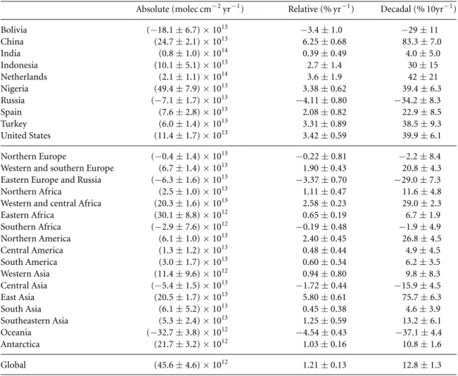
Table 1. Absolute (molec cm−2yr−1), relative (% yr−1) and decadal NH3trends (% 10yr−1) calculated for selected countries and
regions based on national daily average time series (2008–2018) measured by IASI/Metop-A. The relative trend is expressed as compound growth rate from 2008. The regions are shown in figure2(c). TableB1reports trend values for each country.
Absolute (molec cm−2yr−1) Relative (% yr−1) Decadal (% 10yr−1)
Bolivia (−18.1 ± 6.7) × 1013 −3.4 ± 1.0 −29 ± 11 China (24.7± 2.1) × 1013 6.25± 0.68 83.3± 7.0 India (0.8± 1.0) × 1014 0.39± 0.49 4.0± 5.0 Indonesia (10.1± 5.1) × 1013 2.7± 1.4 30± 15 Netherlands (2.1± 1.1) × 1014 3.6± 1.9 42± 21 Nigeria (49.4± 7.9) × 1013 3.38± 0.62 39.4± 6.3 Russia (−7.1 ± 1.7) × 1013 −4.11 ± 0.80 −34.2 ± 8.3 Spain (7.6± 2.8) × 1013 2.08± 0.82 22.9± 8.5 Turkey (6.0± 1.4) × 1013 3.31± 0.89 38.5± 9.3 United States (11.4± 1.7) × 1013 3.42± 0.59 39.9± 6.1 Northern Europe (−0.4 ± 1.4) × 1013 −0.22 ± 0.81 −2.2 ± 8.4
Western and southern Europe (6.7± 1.4) × 1013 1.90± 0.43 20.8± 4.3
Eastern Europe and Russia (−6.3 ± 1.6) × 1013 −3.37 ± 0.70 −29.0 ± 7.3
Northern Africa (2.5± 1.0) × 1013 1.11± 0.47 11.6± 4.8
Western and central Africa (20.3± 1.6) × 1013 2.58± 0.23 29.0± 2.3
Eastern Africa (30.1± 8.8) × 1012 0.65± 0.19 6.7± 1.9 Southern Africa (−2.9 ± 7.6) × 1012 −0.19 ± 0.48 −1.9 ± 4.9 Northern America (6.1± 1.0) × 1013 2.40± 0.45 26.8± 4.5 Central America (1.3± 1.2) × 1013 0.48± 0.44 4.9± 4.5 South America (3.0± 1.7) × 1013 0.60± 0.34 6.2± 3.5 Western Asia (11.4± 9.6) × 1012 0.94± 0.80 9.8± 8.3 Central Asia (−5.4 ± 1.5) × 1013 −1.72 ± 0.44 −15.9 ± 4.5 East Asia (20.5± 1.7) × 1013 5.80± 0.61 75.7± 6.3 South Asia (6.1± 5.2) × 1013 0.45± 0.38 4.6± 3.9 Southeastern Asia (5.3± 2.4) × 1013 1.25± 0.59 13.2± 6.1 Oceania (−32.7 ± 3.8) × 1012 −4.54 ± 0.43 −37.1 ± 4.4 Antarctica (21.7± 3.2) × 1012 1.03± 0.16 10.8± 1.6 Global (45.6± 4.6) × 1012 1.21± 0.13 12.8± 1.3
(see figure3(a)), underlining the urgent need of tak-ing into account meteorological factors in the cur-rent state-of-the-art bottom-up emissions inventor-ies [1]. Declining emissions of acidifying compounds, as much as 62 % in the 2008–2018 period for SOxand
28 % for NOxin EU-28 [89], also increased the
atmo-spheric lifetime of NH3and impacted the trend in the
region [23,91].
In the Middle East, Israel, Jordan and Turkey are characterized by relatively large positive trends over 3 % yr−1, which likely originate from increased emis-sions. For example, Turkey experienced an import-ant intensification of its agricultural production dur-ing the past two decades [92]. During the 2008–2018 period, agricultural use of nitrogen nutrients in the country grew by 2.8 % yr−1 [93], similarly to Israel, while the total anthropogenic emissions increased sharply by 4.8 % yr−1[89]. While Syria shows a mod-erate positive trend, several grid cells around Damas-cus and south of Homs in figure2exhibit a downward trend reflecting the decline of atmospheric emissions due to the civil war that started in 2011 [12]. In northern Africa, only Tunisia and Egypt present sig-nificant positive changes in NH3 columns. The
lat-ter, characterized by an upward trend of 2.39 ±
0.82 % yr−1 due to intensive agriculture in the Nile Delta and River, is known to be the largest fertilizer
consumer in Africa and to have one of the highest nitrogen application rates in the world [94]. Elrys
et al [94] also discusses the strong increase in gaseous
NH3emissions in 2014–2016 following the enhanced
nitrogen use on croplands in the country. Figure2(a) shows that significant increasing trends are also found along the coast of Algeria and especially Morocco, even though for these countries as a whole the trends are not significant.
Western and central Africa are character-ized by a strong upward trend in atmospheric
NH3 total columns that is in absolute terms of
a similar magnitude than east Asia ((20.3 ± 1.6)
× 1013 molec cm−2yr−1), but lower in relative
(2.58± 0.23 % yr−1) (see table 1). This region is dominated by biomass burning emissions associated with agricultural practices [95]. For example, Nigeria
presents an upward trend of 3.38 ± 0.62 % yr−1.
Using the 2008–2017 data record from a previous version of the IASI-NH3dataset, a national increase
of 6 % yr−1 has been reported for the February–
March period which was attributed to agricultural preparation in slash-and-burn cropping systems [96]. In addition, it is worth noting that the agricultural use of nitrogen nutrient in the country increased
strongly by 12 % yr−1 during the 2008–2018 period
Figure 3. Yearly time series expressed in relative terms with respect to 2008 (a) for the world, EU-28, United States, India, China, Turkey and Nigeria and (b) for Bolivia, Russia, Indonesia, Myanmar and Paraguay. The right axis in panel (b) refers to Indonesia only. Regions from tables1are presented in figureB2.
a downward trend of −0.77 ± 0.47 % yr−1. This is
likely related to changes in wetland extent in the Sudd, a vast swamp located in this country [96]. The regional conflict that broke out in 2013 also drastic-ally affected agricultural activities, with a cereal pro-duction reduced by 25 % in 2017 and a drop in live-stock populations [97,98]. The entire eastern Africa presents a very slight upward trend likely driven by increased pyrogenic emissions in the northeastern part of Democratic Republic of the Congo and in the southwestern part of Ethiopia.
The relatively small decadal change in NH3total
columns reported in South America (6.2± 3.5 %)
hides regional and national disparities (figure2). The northwestern coastline, extending from Venezuela to Peru, is the region with the largest positive rates. This is also seen in the EDGAR derived trends, for which these increases relate to agricultural emissions. The growing poultry production along the Peruvian coast is for instance well documented [9]. The posit-ive trend in Brazil is the result of more intense pyro-genic emissions in the central part of the country and, according to EDGAR, increases in anthropo-genic emissions in the southeastern region around Sao Paulo (see figureB4). Jankowski et al [99] also describes how intensification of the Amazon agricul-ture worsens nitrogen pollution. Bolivia and Paraguay exhibit negative trends around−3 % yr−1 related to important biomass burning episodes that occurred in 2010 (figures3(b) and B5).
In the U.S., IASI NH3 columns rose by
3.42± 0.59 % yr−1. This result is in line with the trends obtained from the AIRS satellite (2.6 % yr−1
over 2002–2016 [37]) and from ground-based
meas-urements (e.g. [21]). Modeling studies have provided
evidence that the upward trend of gas-phase NH3in
the U.S. is partly due to reduced SOxand NOx
emis-sions [100,101]. However, it has also been shown that changing meteorological factors (e.g. drought, tem-perature) play a role in the increase of NH3
concen-trations in the region [101,102]. Reported national emissions decreased from 2008 to 2014 by 3.4 % yr−1, but showed an upturn in the following years to reach the same level in 2017–2018 as in 2008 [103]. At the state scale, the National Emissions Inventory (NEI) from the Environmental Protection Agency (EPA) reports a generally increasing emission trend in the western states, but a declining trend in the central-eastern states [104]. Satellite observations present nonetheless a positive trend over the entire country (figures2(a) and (b)). The peak in 2012 in figure3(a) could be related to higher temperatures in the sum-mer and a related increase in NH3volatilization from
soils, as reported for NOx soil emissions [101]. At
present, NH3plays a key role in nitrogen deposition in
the country (contributing up to 65 % in some places), and these deposition fluxes will be difficult to mitig-ate without reducing emissions [105]. A significant positive trend of 1.53± 0.83 % yr−1is also measured in Canada (note that Yamanouchi et al [106] recently reported a trend of 8.38± 0.77 % yr−1at the city scale of Toronto using the same IASI dataset). While the national emission inventory reports more or less con-stant anthropogenic emissions over the 2008–2018 period [107], biomass burning sustains the increas-ing trend in NH3total columns at northern latitudes
[108,109]. EDGAR presents a pronounced
discon-tinuity between the trend reported for the U.S. and Canada (figureB4).
The calculated trends for Australia are in relat-ive terms quite large at−4.53 ± 0.45 % yr−1. It is however important to note that in absolute terms this decline is almost negligible and artificial. In fact,
inspection of figure 2 shows declines below 0.5×
1015molec cm−2yr−1in most of the Southern
hemi-sphere at the latitude of Australia. These could be related to the misclassification of clouds during the early 2008–2018 period (see section 2.1 and [59]),
or due to an imperfect CO2 trend correction (see
appendixA). For the same reason, trends in
Argen-tina, Chile and South Africa are to be interpreted with caution. The trends over the ice sheets of Antarctica and Greenland are spurious, and exacerbated by the general poorer performance of the NH3retrieval over
cold surfaces (see again appendixA).
From the national trends we have calculated a worldwide decadal increase in atmospheric NH3total
columns of 12.8± 1.3 %, which corresponds to a pos-itive growth rate of 1.21 ± 0.13 % yr−1. Note that
Figure 4. (Top) Yearly time series of NH3emissions reported for the Netherlands in the framework of the Gothenburg Protocol
(1990–2018, Gg yr−1, black), NH3surface concentrations from the LML (1993–2018, µg m−3, orange) and from the MAN
network (2005–2018, µg m−3, dashed orange). 27 MAN stations (6, 8, 9, 11, 12, 20, 21, 23, 32, 35, 39, 45, 46, 54, 58, 61, 63, 65, 68, 84, 87, 88, 121, 122, 130, 131, 990) and 8 LML stations (131, 235, 444, 538, 633, 722, 738, 929) have been considered. (Bottom) Yearly NH3time series for the Netherlands measured by IASI (molec cm−2, blue) and at the surface by ground-based instruments
from the LML network (µg m−3, orange). Only the LML stations with data coverage over the entire 2008–2018 period have been used (stations 131, 444, 538, 633, 738).
these numbers are for land only. Trends over coastal areas follow in general those observed over the nearby land regions located upwind. For example, a signi-ficant positive trend in transported NH3 is clearly
identifiable in the Gulf of Guinea (southern coast of western Africa), in the Yellow Sea (east coast of China) and in the Caribbean Sea (northern coast of Colombia). Conversely, following the decline in NH3
total columns observed in southeastern India, a neg-ative trend is calculated over the Bay of Bengal and the Arabian Sea.
4. Case study: the Netherlands
The Netherlands was one of the first countries
world-wide to implement NH3 abatement measures in the
1980s. This included regulation of manure applica-tion rates, introducing the mineral accounting sys-tem, introduction of emission poor housing systems, manure storage coverage and injection of manure in the soil. Since the early 1990s, NH3 is measured
hourly at eight locations in the country from the ground-based stations of the National Air Quality Monitoring Network (or LML standing for ‘Lan-delijk Meetnet Luchtkwaliteit’), which was set up
to monitor the Dutch NH3 emissions abatement
policies [22,110]. In 2005, the LML network was
extended by measurements with passive samplers in the Measuring Ammonia in Nature (MAN) network
to follow the NH3 concentrations in nature areas
[111,112].
More than 20 years ago, a discrepancy was
observed between these NH3 measurements and
expected levels derived from estimated NH3
emis-sions in the Netherlands [113]. Different reasons were found for this mismatch: (a) a changing chemical
cli-mate which affected the conversion rate of NH3 to
NH+4; (b) a reduction of acidifying compounds such
as SO2 and NOx both in the atmosphere as well as
on the surface leading to more NH3 in the
atmo-sphere; (c) less effective abatement measures in prac-tice as compared to measured lab reductions; (d) fraud with manure transports and (e) the contribu-tion of unknown sources such as the sea and the sen-escence of leaves [114–116].
LML NH3concentrations measured at the surface
show a downward trend of 36 % for the 1993–2004 period, while an upward trend of 19 % is repor-ted for 2005–2014 [22]. In contrast, the official NH3
emissions reported in the framework of the Gothen-burg Protocol decreased for the entire period in the Netherlands and are currently 63.1 % lower than in 1990, even though since 2010, these have leveled off [89]. This is illustrated in the top panel
of figure4which shows the evolution of the
repor-ted emissions (1990–2018, Gg yr−1, black) as well
as yearly NH3surface concentrations from the LML
(1992–2018, µg m−3, orange) and the MAN network
(2005–2018, µg m−3, dashed orange). van Zanten
et al [22] have shown that the comparison between the emission and concentration trend improves when
the influence of meteorological conditions on the concentrations is taken into account.
Using 11 years (2008–2018) of IASI satellite
daily observations of NH3 columns, we calculate an
increasing trend of 3.6± 1.9 % yr−1 in the Nether-lands. Over the same time-period, the daily ground-based NH3concentrations measured at five LML sites
exhibit a consistent 2.5± 0.5 % yr−1growth rate. The
bottom panel of figure 4 presents the annual NH3
time series for IASI/Metop-A (molec cm−2, blue),
IASI/Metop-B (molec cm−2, dashed blue) and LML
(µg m−3, orange). A sharp increase in the annual
mean is measured in 2018, due to the exceptionally warm, sunny and dry weather conditions during that year, as NH3 volatilization strongly increases with
temperature and as deposition rates are lower when it is drier [1,86–88].
In 2018, the European Court of Justice advised that the current Dutch legislation was not strict enough to protect Natura 2000 areas from nitrogen deposition [117], as required by the European Hab-itat Directive (EHD) (directive 92/43/EEG). This led to several rulings by the Dutch Council of State in 2019, putting on hold more than 18 000 projects on building houses and roads and in the agricultural sec-tor and thus leading to the ‘Dutch Nitrogen crisis’. The proposed policy to halve the country’s livestock pop-ulation to reduce nitrogen deposition caused massive
demonstrations from farmers [44]. A special
com-mission was put in place, the Comcom-mission Remkes, to advice about the long-term policies to reduce nitro-gen. They recommended that emissions should be reduced by 50 % in 10 years to protect 75 % of the Natura 2000 against excess nitrogen deposition and that on a local scale, further reductions are necessary.
5. Conclusions
Using the data record from the IASI sounder we have obtained and characterized the evolution of atmo-spheric NH3 at global, regional and national scales
from 2008 to 2018. We have reported large increases of NH3in several subcontinental regions over the last
decade, especially in east Asia (75.7± 6.3 %) but also
in western and central Africa (29.0± 2.3 %), North
America (26.8± 4.5 %) and western and southern
Europe (20.8± 4.3 %). The upward trends observed
in many countries can be attributed to a combina-tion of increasing emissions and a longer residence time of NH3in the atmosphere due to declining
emis-sions of sulfur and nitrogen oxides. Regions domin-ated by biomass burning emissions exhibit decreasing or increasing trends depending on when the strongest events took place. Apart from declines related to fires, notable declines were also found in the southwestern part of India and central Asia.
In view of the major role of NH3 for the loss
of biodiversity, for air quality and human health, emissions need to be reduced urgently. A series of
options exists to control the loss of NH3 from
agri-cultural activities to the atmosphere (e.g. [118]).
Lim-iting these atmospheric NH3losses would also have
co-benefits for our climate [119]. Recent studies have
shown that the abatement costs to reduce NH3
emis-sions is much lower than the economical and societal benefits (see [120] for Europe and [121] for China), which should trigger our willingness for action. Cur-rent and planned infrared satellite missions provide the necessary observational means to monitor the effect of implemented policies (e.g. [122, 123]) to support the goals of the Sustainable Nitrogen Man-agement resolution (UNEP/EA.4/Res.14) adopted by the United Nations Environment Assembly on 15 March 2019 [124].
Data availability statement
The IASI-NH3 datasets are available from the Aeris
data infrastructure (http://iasi.aeris-data.fr/NH3). It is also planned to be operationally distributed by EUMETCast under the auspices of the EUMETSAT Atmospheric Monitoring Satellite Application Facil-ity (AC-SAF;http://ac-saf.eumetsat.int).
Acknowledgments
IASI has been developed and built under the
respons-ibility of the Centre National d’´Etudes Spatiales
(CNES, France). It is flown on board the Metop satel-lites as part of the EUMETSAT Polar System. The IASI L1c data are received through the EUMETCast near real-time data distribution service. National and regional maps have been made with Natural Earth (naturalearthdata.com). The research was funded by the F.R.S.-FNRS and the Belgian State Federal Office for Scientific, Technical and Cultural Affairs (Pro-dex arrangement IASI.FLOW). M Van Damme is Postdoctoral Researcher (Chargé de Recherche) and L Clarisse is Research Associate (Chercheur Quali-fié) both supported by the Belgian F.R.S.-FNRS. M A Sutton acknowledges support from the Global Envir-onment Facility (GEF) through the UN Environ-ment Programme for the Towards INMS project. C Clerbaux is grateful to CNES for scientific collab-oration and financial support.
Appendix A. Version 3 ANNI-NH
3product
The ANNI-NH3-v3 IASI product builds on the
her-itage of version 1 [52], version 2 [53], and recent improvements in the neural network (NN) retrieval setup introduced in Franco et al [54] for the retrieval of volatile organic compounds (VOCs). We refer to the above-mentioned papers for a detailed descrip-tion of the retrieval methodology. The specific changes from v2.2 to v3 for NH3are outlined in detail
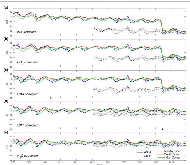
Figure A1. IASI/Metop-A (solid lines) and IASI/Metop-B (dashed lines) NH3Hyperspectral Range Index (HRI, no unit) monthly
time series over three remote locations: North Atlantic Ocean (20◦N–40◦N; 30◦W–60◦W), Pacific Ocean (0◦S–30◦S; 125◦ W–175◦W) and Indian Ocean (5◦S–25◦S; 55◦E–95◦E). From top to bottom: (a) not corrected time series and successive implementation of corrections (b)–(e).
A.1. Changes to the HRI and debiasing procedures The Hyperspectral Range Index (HRI) has been set up following the iterative procedure outlined in [54]. The spectral range has been slightly reduced
(812–1126 cm−1) to minimize interferences from
other species and/or local variation in surface emissivity. The end result is that the HRI is more sensitive to NH3and less affected by interferences.
Analysing the initial time series of the mean HRI over remote oceans, we noticed (a) offsets that coin-cided with changes to the IASI instrument, (b) a slowly decreasing trend and (c) a residual dependence on H2O. In the rest of the section we outline the first
order corrections that were introduced to account for all of these.
The declining trend over remote areas that was identified in the HRI of NH3is apparent in the top
panel of figureA1. As the trend is linear, and as there
are a couple of weak CO2 absorption bands in the
812–1126 cm−1 spectral range, this trend is most
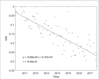
likely due to the ever increasing concentrations of CO2. To correct this bias, we analyzed monthly
aver-aged HRI from IASI spectra measured over a remote
location in the Pacific Ocean (17◦N–22◦N; 153◦W– 158◦ W) versus time (figureA2). The linear
regres-sion (y =−8.69 × 10⁻⁵x + 63.75, r =−0.84, with x
and y being the time (in months) and the HRI (no unit), respectively) models the relationship well and was therefore used to apply a first-order correction to the calculated HRI.
On 7 June 2017, a minor change in the con-figuration parameters for the apodization function of IASI/Metop-A instrument had a clear impact
on the calculated HRI (figure A1, panels (a)–(c)).
This recalibration made IASI/Metop-A more in line with IASI/Metop-B instrument. As the HRI is based on a covariance matrix from spectra of the year 2013, the HRI calculated after the recalibration for IASI/Metop-A have to be adjusted, as well as the entire time series of IASI/Metop-B. Comparison of the HRI values on 6 June with the ones from 8 June 2017, revealed a temperature dependence in the off-set. A satisfactory correction was obtained using a linear regression (y =−3.5 × 10⁻³x− 0.69, r = 0.89,
with x being the temperature of the baseline (in K) and y the median of the HRI difference between
Figure A2. HRI (no unit) monthly time series over a remote location in the Pacific Ocean. The linear regression is indicated in black.
the 6 and the 8 June 2017 (no unit); see figureA1, panel (d)).
Another change in the IASI Level 1C occurred on
18 May 2010 [125] and corresponds to an
improve-ment of the spectral calibration [126]. An empirical correction was introduced as a function of latitude and day of the year. The precise offsets were computed as the difference between the median HRI calculated before and after the 18 May 2010, the median being calculated in 1◦latitude bins from all the HRI with an absolute longitude above 160◦and an absolute value below 5. This difference was calculated for each day of the year and applied to the HRI calculated before the 18 May 2010 (figureA1, panel (c)).
Finally, a H2O correction similar to the one
applied in the previous ANNI–NH3version (already
described in [53]) was implemented. This does not change the behavior of the HRI over time, but helps to de-bias it (i.e. after the correction, the mean HRI over remote oceans is closer to zero). Panel (e) of figureA1presents the corrected monthly time series of HRI over three remote locations. It shows that the corrections allow us to obtain a coherent time series over the IASI operating period, centered around zero and as expected without noticeable jumps or trends. A.2. Changes to the neural network architecture and training
The following series of changes have been introduced:
• The size of the network was increased from one
computational layer of 15 neurons [52] to two lay-ers of 12 nodes.
• In terms of input variables, similarly to the
treat-ment of VOCs [54], we now use a coarse H2O
profile as input to the network, as opposed to the total column that was used before. In addition, three extra temperature levels are introduced in the lower troposphere (at 0.5, 1.5 and 2.5 km above the surface). Especially in the evening, when thermal
inversion can occur, it is expected that this change results in a more accurate retrieval. Finally, the sur-face temperature is kept as an input parameter to the network instead of a baseline temperature used for the VOCs.
• The range of thermal contrast situations in the
training set was artificially increased to better train the network. In addition, the total num-ber of samples in the training set increased from 450 000 to close to 500 000 (also because now two networks are trained, as explained in the next point).
• Similarly to the previous versions of the NN
retrieval of NH3, the vertical profile of NH3 was
parameterized with a Gaussian function for the for-ward simulations. It is now defined as:
NH3(vmr) = ScalFact· e−(
(z−z0)2
2σ2 ). (A1)
Two different training sets have been built: (a) One representative for observations close to
emission sources (thus with the peak con-centration at the surface), where z0was fixed
to 0 km and where sigma (σ) was assigned a random number between 100 m and 6 km.
(b) One representative for transported NH3,
with a peak concentration above the sur-face. Here z0was assigned a random number
between 0 and 20 km.
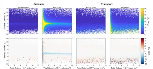
• The training performance is evaluated in figureA3
and shows similar good performances as in the pre-vious versions.
A.3. Changes to the input data and post-filtering
• As before, IASI L2 data is used as meteorological
inputs to the network, and the resulting near-real
time (NRT) NH3 product is called ANNI–NH3
-v3. A second reanalysis product, ANNI-NH3-v3R,
is also available. This dataset was produced with the same neural networks, but instead of the IASI L2 data, reanalyzed ERA5 data was used as met-eorological inputs [58]. Note that ANNI-NH3-v2R
still used the ERA-Interim data. ERA5, compared to ERA-Interim, has much improved meteorology and is available on an hourly timescale with a 0.28125◦resolution.
• Observations above land are standard retrieved
using the neural network for source areas (emis-sion network), with as σ value the collocated ERA5 boundary layer height for v3R (see [52]). For the NRT product v3, we used as input for σ a monthly climatology based on over 10 years of ERA5 data (from October 2007 to December 2018). For obser-vations above the ocean, we assume z0=1.4 km and
σ =1.28/√2 (see again [52]).
• The condition on the ratio in the post-filter (see
Figure A3. Performance evaluation (top: error, bottom: bias, both in %) of the emission network (left four panels) and transport network (right four panels), with and without adding noise. Note that compared to the evaluation plots in [53], the median value is shown in each grid box, which removes the effect of outliers and allows us to better assess the real performance of the network.
Figure A4. (Top to bottom, left to right) v2.2, v2.2R-Interim, v3, v3R-ERA5 10-year averaged NH3total columns distributions
(mol cm−2) based on IASI/Metop-A measurements from 1 January 2008 to 31 December 2017 (morning overpasses) on a 0.25◦
× 0.25◦grid.
much as possible ‘good observations’, while remov-ing those with a very large uncertainty. In
partic-ular, the threshold value on the ratio NH3/HRI
is now 1.5 × 10¹⁶ mol cm−2 instead of 1.75 ×
1016molec cm−2 (so slightly more measurements
are retained). A.4. Example
Overall and on average, the v3 does not differ significantly from v2, although differences can be large on individual observations: for columns above
4× 10¹⁵molec cm−2, 80 % of the data agree to within
20 % [62]. As an illustration, figureA4presents the
IASI-NH3 10-year averaged distributions from the
four datasets (v2.2, v2.2R, v3 and v3R). The averaged columns are slightly larger in the reanalyzed versions, and higher for v3 than for v2. One notable regression in v3 is the performance over ice sheets at high
latit-ude, which yield a larger mean NH3column than in
v2.2. This is likely related to the fact that the current post-filter is less stringent and was tuned for the trop-ics and mid-latitudes.
Appendix B. Figures and tables
Figure B1.Temporal NH3trend (molec cm−2yr−1) calculated from IASI-NH3daily time series (2008–2018) in each 0.5◦× 0.5◦
cell and based on the bootstrap method. Cells with non-significant trend have been stippled.
Figure B2. Yearly time series expressed in relative terms with respect to 2008 for the regions presented in table1. (a) Northern Europe, Western and southern Europe, Eastern Europe and Russia, Northern Africa, Western and central Africa, Eastern Africa, Southern Africa and Oceania. (b) Northern America, Central America, South America, Western Asia, Central Asia, East Asia, South Asia, Southeastern Asia and Antarctica.
Figure B3. Bootstrap (green and red) and standard least squares linear regression (dashed yellow) fit applied on (daily and yearly, respectively) IASI-NH3time series (blue, molec cm−2). National absolute (molec cm−2yr−1) and relative (% yr−1) NH3trend
and decadal relative change (% 10yr−1) based on national daily time series (2008–2018) measured by IASI/Metop-A are indicated as inset in the top-left corner of each subpanel.
Figure B4. NH3emission trend (g m−2yr−1) based on Emission Database for Global Atmospheric Research (EDGAR) v5.0
yearly time series during the 2008–2015 period. The trends have been calculated using a standard least squares linear regression fit applied on the yearly data [6].
Figure B5. NH3emission trend (g m−2yr−1) based on Global Fire Emissions Database (GFED) v4.1s yearly time series during
the 2008–2018 period. The trends have been calculated using a standard least squares linear regression fit applied on the yearly data [8].
Table B1. National absolute (molec cm−2yr−1), relative (% yr−1) and decadal NH3trends (% 10yr−1) based on national daily time
series (2008–2018) measured by IASI/Metop-A. The relative trend is expressed as compound grow rate from 2008. Countries for which the calculated trend is significant are in bold.
Absolute (molec cm−2yr−1) Relative (% yr−1) Decadal (% 10yr−1)
Afghanistan (−1.3 ± 2.5) × 1013 −0.46 ± 0.85 −4.5 ± 8.8 Albania (−2.5 ± 5.5) × 1013 −1.2 ± 2.4 −12 ± 26 Algeria (0.2± 1.9) × 1013 0.07± 0.84 0.7± 8.7 Angola (9.4± 2.3) × 1013 2.57± 0.69 28.9± 7.1 Antarctica (21.7± 3.2) × 1012 1.03± 0.16 10.8± 1.6 Argentina (−13.7 ± 2.7) × 1013 −3.50 ± 0.58 −30.0 ± 6.0 Armenia (−5.6 ± 3.7) × 1013 −1.8 ± 1.1 −17 ± 11 Australia (−31.6 ± 3.9) × 1012 −4.53 ± 0.45 −37.1 ± 4.6 Austria (3.0± 5.2) × 1013 1.0± 1.7 10± 18 Azerbaijan (−11.0 ± 4.7) × 1013 −1.74 ± 0.67 −16.1 ± 6.9 Bahamas (−5.5 ± 5.6) × 1013 −14.3 ± 6.0 −79 ± 80 Bangladesh (−4.9 ± 2.0) × 1014 −2.24 ± 0.80 −20.3 ± 8.3 Belarus (3.1± 8.7) × 1013 0.9± 2.3 9± 25 Belgium (21.0± 9.9) × 1013 4.2± 2.2 50± 24 Belize (−9.0 ± 8.5) × 1013 −4.2 ± 2.9 −35 ± 33 Benin (5.9± 1.2) × 1014 3.64± 0.85 43.0± 8.8 Bhutan (−1.8 ± 8.0) × 1013 −0.6 ± 2.3 −6 ± 26 Bolivia (−18.1 ± 6.7) × 1013 −3.4 ± 1.0 −29 ± 11
Bosnia and Herz. (−1.8 ± 5.5) × 1013 −0.9 ± 2.2 −8 ± 25
Botswana (0.6± 2.1) × 1013 0.28± 0.90 2.8± 9.4 Brazil (12.1± 3.1) × 1013 1.94± 0.53 21.2± 5.4 Bulgaria (0.9± 4.2) × 1013 0.4± 1.8 4± 20 Burkina Faso (34.6± 8.4) × 1013 3.16± 0.85 36.5± 8.8 Burundi (23.4± 6.4) × 1013 2.86± 0.85 32.6± 8.9 Cabo Verde (−0.7 ± 7.8) × 1013 −0.2 ± 2.0 −2 ± 22 Cambodia (17.3± 4.8) × 1013 4.2± 1.3 51± 14 Cameroon (36.3± 7.8) × 1013 3.54± 0.87 41.6± 9.0 Canada (2.9± 1.5) × 1013 1.53± 0.83 16.4± 8.6
Central African Rep. (4.7± 6.4) × 1013 0.47± 0.64 4.8± 6.5
Chad (10.4± 4.1) × 1013 2.08± 0.86 22.8± 9.0
Chile (−60.7 ± 8.4) × 1012 −11.35 ± 0.93 −70.0 ± 9.7
People’s Republic of China (24.7± 2.1) × 1013 6.25± 0.68 83.3± 7.0
Colombia (10.7± 4.0) × 1013 2.8± 1.1 32± 12 Congo (2.9± 1.0) × 1014 3.8± 1.4 45± 15 Costa Rica (2.8± 4.5) × 1013 2.6± 4.0 30± 47 Cote d’Ivoire (42.5± 9.2) × 1013 2.83± 0.68 32.2± 7.0 Croatia (4.5± 5.5) × 1013 1.4± 1.7 15± 18 Cuba (−5.2 ± 2.0) × 1013 −4.8 ± 1.4 −39 ± 15 Cyprus (12.2± 5.7) × 1013 3.6± 1.9 43± 20 Czechia (3.7± 6.2) × 1013 1.1± 1.8 12± 20
Dem. Rep. Congo (29.4± 5.8) × 1013 3.16± 0.70 36.5± 7.3
Denmark (11.5± 7.7) × 1013 3.9± 2.7 46± 31 Djibouti (0.2± 4.0) × 1013 0.1± 1.6 1± 17 Dominican Rep. (0.9± 2.8) × 1013 0.8± 2.3 8± 25 Ecuador (9.4± 3.7) × 1013 3.9± 1.7 47± 18 Egypt (5.8± 1.9) × 1013 2.39± 0.82 26.6± 8.6 El Salvador (3.7± 4.5) × 1013 1.5± 1.8 16± 19 Eritrea (0.7± 2.9) × 1013 0.3± 1.1 3± 11 Estonia (−3.0 ± 7.7) × 1013 −1.9 ± 3.8 −18 ± 45 Eswatini (−5.8 ± 4.9) × 1013 −3.3 ± 2.2 −29 ± 25 Ethiopia (1.8± 2.0) × 1013 0.34± 0.38 3.5± 3.9 Fiji (−3.1 ± 6.1) × 1013 −2.9 ± 4.2 −25 ± 51 Finland (−5.8 ± 4.1) × 1013 −4.5 ± 2.3 −37 ± 26 France (7.4± 3.4) × 1013 2.1± 1.0 24± 11 Gabon (29.3± 9.7) × 1013 4.6± 1.7 56± 19 Gambia (1.1± 1.3) × 1014 1.0± 1.1 10± 12 Georgia (−0.9 ± 4.4) × 1013 −0.3 ± 1.3 −3 ± 14 Germany (8.9± 5.1) × 1013 2.1± 1.2 23± 13 Ghana (5.6± 1.2) × 1014 3.28± 0.77 38.1± 8.0
Table B1. (Continued.)
Absolute (molec cm−2yr−1) Relative (% yr−1) Decadal (% 10yr−1)
Greece (−2.6 ± 3.0) × 1013 −1.5 ± 1.5 −14 ± 16 Greenland (−23.0 ± 7.3) × 1012 −1.11 ± 0.33 −10.5 ± 3.3 Guatemala (−7.9 ± 4.5) × 1013 −2.8 ± 1.3 −25 ± 14 Guinea (23.8± 7.5) × 1013 1.96± 0.65 21.4± 6.7 Guinea-Bissau (−0.1 ± 1.5) × 1014 −0.1 ± 1.1 −1 ± 12 Guyana (−0.8 ± 4.4) × 1013 −0.4 ± 2.1 −4 ± 23 Haiti (1.5± 3.3) × 1013 0.9± 1.9 9± 21 Honduras (−5.5 ± 4.0) × 1013 −3.3 ± 1.9 −28 ± 20 Hungary (7.5± 5.4) × 1013 2.0± 1.5 22± 16 Iceland (−6.4 ± 4.1) × 1013 −6.2 ± 2.7 −47 ± 30 India (0.8± 1.0) × 1014 0.39± 0.49 4.0± 5.0 Indonesia (10.1± 5.1) × 1013 2.7± 1.4 30± 15 Iran (−4.1 ± 1.2) × 1013 −3.71 ± 0.89 −31.5 ± 9.3 Iraq (4.5± 3.7) × 1013 2.5± 2.1 28± 23 Ireland (0.6± 5.5) × 1013 0.4± 3.2 4± 37 Israel (17.4± 4.9) × 1013 4.6± 1.5 56± 16 Italy (9.5± 3.2) × 1013 2.26± 0.82 25.0± 8.5 Jamaica (−1.8 ± 5.6) × 1013 −1.6 ± 3.8 −15 ± 45 Japan (8.3± 2.9) × 1013 7.7± 3.3 110± 38 Jordan (8.0± 3.1) × 1013 4.1± 1.8 50± 19 Kazakhstan (−4.1 ± 1.9) × 1013 −1.76 ± 0.71 −16.2 ± 7.3 Kenya (5.4± 2.4) × 1013 1.14± 0.52 12.0± 5.3 Kosovo (−1.3 ± 6.3) × 1013 −0.6 ± 2.7 −6 ± 30 Kuwait (6.7± 7.2) × 1013 5.9± 6.2 77± 83 Kyrgyzstan (−4.8 ± 3.9) × 1013 −0.97 ± 0.74 −9.3 ± 7.6 Laos (2.1± 5.4) × 1013 0.5± 1.2 5± 13 Latvia (−1.5 ± 7.9) × 1013 −0.7 ± 3.2 −7 ± 36 Lebanon (7.6± 4.7) × 1013 3.7± 2.5 44± 28 Lesotho (−0.7 ± 2.4) × 1013 −1.4 ± 3.6 −13 ± 42 Liberia (4.2± 1.6) × 1014 2.7± 1.1 30± 12 Libya (−1.0 ± 1.4) × 1013 −0.71 ± 0.97 −7 ± 10 Lithuania (4.5± 8.3) × 1013 1.5± 2.7 17± 30 Macedonia (−5.5 ± 4.6) × 1013 −4.0 ± 2.5 −33 ± 28 Madagascar (−1.0 ± 1.4) × 1013 −0.65 ± 0.81 −6.3 ± 8.4 Malawi (5.2± 3.1) × 1013 1.42± 0.88 15.2± 9.1 Malaysia (1.7± 6.1) × 1013 0.6± 1.9 6± 21 Mali (6.7± 4.5) × 1013 1.28± 0.87 13.6± 9.0 Mauritania (−0.8 ± 3.9) × 1013 −0.2 ± 1.2 −2 ± 12 Mexico (2.5± 1.5) × 1013 0.81± 0.51 8.4± 5.2 Moldova (4.1± 5.5) × 1013 1.2± 1.6 13± 17 Mongolia (−4.9 ± 1.6) × 1013 −3.22 ± 0.86 −27.9 ± 9.0 Montenegro (−6.7 ± 8.5) × 1013 −3.9 ± 3.5 −32 ± 41 Morocco (1.3± 2.0) × 1013 0.52± 0.80 5.3± 8.3 Mozambique (0.6± 2.4) × 1013 0.20± 0.83 2.1± 8.7 Myanmar (−18.9 ± 5.0) × 1013 −3.19 ± 0.70 −27.7 ± 7.3 N. Cyprus (20.2± 5.8) × 1013 5.7± 1.9 74± 21 Namibia (−0.2 ± 1.6) × 1013 −0.10 ± 0.85 −0.9 ± 8.8 Nepal (−1.4 ± 1.1) × 1014 −1.27 ± 0.89 −12.0 ± 9.2 Netherlands (2.1± 1.1) × 1014 3.6± 1.9 42± 21 New Caledonia (−5.8 ± 5.2) × 1013 −13.8 ± 5.4 −77 ± 70 New Zealand (−6.5 ± 2.4) × 1013 −4.7 ± 1.4 −38 ± 14 Nicaragua (−0.3 ± 4.2) × 1013 −0.2 ± 2.5 −2 ± 28 Niger (10.1± 4.4) × 1013 2.4± 1.1 26± 11 Nigeria (49.4± 7.9) × 1013 3.38± 0.62 39.4± 6.3 North Korea (33.8± 6.5) × 1013 14.7± 4.6 295± 57 Norway (−0.3 ± 2.0) × 1013 −0.2 ± 1.2 −2 ± 13 Oman (−5.9 ± 4.0) × 1013 −7.3 ± 3.1 −53 ± 36 (Continued)
Table B1. (Continued.)
Absolute (molec cm−2yr−1) Relative (% yr−1) Decadal (% 10yr−1)
Pakistan (3.8± 1.5) × 1014 1.86± 0.78 20.2± 8.1
Palestine (25.0± 7.0) × 1013 4.8± 1.6 60± 17
Panama (10.0± 6.0) × 1013 5.2± 3.4 67± 40
Papua New Guinea (1.0± 3.7) × 1013 0.6± 2.2 6± 24
Paraguay (−2.8 ± 1.3) × 1014 −2.8 ± 1.1 −25 ± 12 Peru (7.3± 2.1) × 1013 2.44± 0.75 27.2± 7.8 Philippines (2.7± 3.2) × 1013 1.2± 1.4 13± 15 Poland (8.6± 4.9) × 1013 2.4± 1.4 27± 15 Portugal (5.4± 4.8) × 1013 2.1± 1.9 23± 21 Puerto Rico (0.7± 5.7) × 1013 0.7± 5.2 8± 66 Romania (0.4± 4.2) × 1013 0.1± 1.3 1± 13 Russia (−7.1 ± 1.7) × 1013 −4.11 ± 0.80 −34.2 ± 8.3 Rwanda (32.4± 6.0) × 1013 4.04± 0.86 48.6± 9.0 S. Sudan (−8.4 ± 5.5) × 1013 −0.77 ± 0.47 −7.4 ± 4.8 Saudi Arabia (0.2± 1.8) × 1013 0.5± 3.3 5± 39 Senegal (9.5± 8.7) × 1013 0.95± 0.87 9.9± 9.1 Serbia (1.6± 5.1) × 1013 0.5± 1.5 5± 16 Sierra Leone (2.3± 1.5) × 1014 1.40± 0.92 14.9± 9.6 Slovakia (6.2± 5.9) × 1013 2.1± 2.0 23± 22 Slovenia (7.9± 7.9) × 1013 2.4± 2.4 27± 27 Solomon Is. (0.1± 9.9) × 1013 0.1± 6.2 1± 83 Somalia (−4.6 ± 1.8) × 1013 −2.26 ± 0.78 −20.4 ± 8.1 Somaliland (−5.2 ± 2.4) × 1013 −2.38 ± 0.93 −21.4 ± 9.7 South Africa (−7.3 ± 8.0) × 1012 −0.70 ± 0.72 −6.8 ± 7.5 South Korea (48.1± 7.0) × 1013 14.6± 3.6 291± 42 Spain (7.6± 2.8) × 1013 2.08± 0.82 22.9± 8.5 Sri Lanka (−12.8 ± 5.2) × 1013 −4.6 ± 1.4 −37 ± 15 Sudan (6.9± 3.2) × 1013 2.2± 1.1 25± 11 Suriname (1.2± 5.1) × 1013 0.5± 2.1 6± 23 Sweden (−0.0 ± 2.7) × 1013 −0.0 ± 1.6 −0 ± 18 Switzerland (4.9± 5.5) × 1013 1.7± 1.8 18± 20 Syria (3.9± 3.2) × 1013 1.6± 1.3 17± 14 Taiwan (20.8± 7.0) × 1013 4.0± 1.5 49± 16 Tajikistan (−12.9 ± 4.0) × 1013 −2.74 ± 0.73 −24.3 ± 7.6 Tanzania (11.2± 3.1) × 1013 1.98± 0.59 21.7± 6.1 Thailand (12.3± 4.5) × 1013 2.15± 0.84 23.8± 8.7 Timor-Leste (−1.3 ± 5.1) × 1013 −1.0 ± 3.3 −10 ± 38 Togo (5.9± 1.3) × 1014 3.41± 0.87 39.9± 9.1 Tunisia (7.6± 3.8) × 1013 1.74± 0.90 18.8± 9.4 Turkey (6.0± 1.4) × 1013 3.31± 0.89 38.5± 9.3 Turkmenistan (−11.0 ± 3.7) × 1013 −2.55 ± 0.74 −22.8 ± 7.6 Uganda (21.2± 4.5) × 1013 2.18± 0.50 24.0± 5.1 Ukraine (−3.6 ± 4.2) × 1013 −1.2 ± 1.2 −11 ± 13
United Arab Emirates (−4.9 ± 4.6) × 1013 −6.5 ± 3.9 −49 ± 46
United Kingdom (6.1± 4.5) × 1013 2.9± 2.2 33± 24
United States of America (11.4± 1.7) × 1013 3.42± 0.59 39.9± 6.1
Uruguay (−8.0 ± 7.3) × 1013 −1.7 ± 1.4 −16 ± 14
Uzbekistan (−5.4 ± 6.0) × 1013 −0.96 ± 0.98 −9 ± 10
Vanuatu (6.9± 9.5) × 1013 13± 15 (2.3± 3.1) × 102
Venezuela, Bolivarian Republic of (1.2± 2.6) × 1013 0.42± 0.86 4.3± 9.0
Vietnam (17.9± 4.3) × 1013 4.4± 1.2 54± 13
W. Sahara (0.5± 3.7) × 1013 0.5± 3.5 6± 41
Yemen (−2.0 ± 2.1) × 1013 −2.8 ± 2.3 −25 ± 26
Zambia (7.9± 2.2) × 1013 2.20± 0.66 24.3± 6.8