HAL Id: hal-01304938
https://hal.archives-ouvertes.fr/hal-01304938
Submitted on 16 Aug 2016
HAL is a multi-disciplinary open access
archive for the deposit and dissemination of
sci-entific research documents, whether they are
pub-lished or not. The documents may come from
teaching and research institutions in France or
abroad, or from public or private research centers.
L’archive ouverte pluridisciplinaire HAL, est
destinée au dépôt et à la diffusion de documents
scientifiques de niveau recherche, publiés ou non,
émanant des établissements d’enseignement et de
recherche français ou étrangers, des laboratoires
publics ou privés.
Simulation of 3D karst conduits with an object-distance
based method integrating geological knowledge
Guillaume Rongier, Pauline Collon-Drouaillet, Marco Filipponi
To cite this version:
Guillaume Rongier, Pauline Collon-Drouaillet, Marco Filipponi. Simulation of 3D karst conduits with
an object-distance based method integrating geological knowledge. Geomorphology, Elsevier, 2014,
217, pp.152-164. �10.1016/j.geomorph.2014.04.024�. �hal-01304938�
Geomorphology, 217: 152–164, 2014
10.1016/j.geomorph.2014.04.024
Simulation of 3D karst conduits with an object-distance
based method integrating geological knowledge
Guillaume Rongier
1, Pauline Collon
1, and Marco Filipponi
2 1GeoRessources (UMR 7359, Université de Lorraine/ CNRS / CREGU), Vandoeuvre-lès-Nancy, F-54518 France2Bauen im Karst, Alte Spinnerei, CH-8877 Murg, Switzerland
Abstract Karst conduit shapes have a high influence on fluid flows. As these underground hidden sys-tems are partially inaccessible, their stochastic simulation is an essential tool to assess the uncertainties related to these highly exploited water resources. The Object-Distance Simulation Method (ODSIM) is a hybrid dual-scale approach that has been recently proposed to model geological underground struc-tures due to late processes such as dolomitized rocks, mineralized veins or karsts. Using a perturbed Euclidean distance field around a curve representing roughly the conduit centre and called a skeleton, the resulting shapes are globally cylindrical-like 3D envelopes. But at a drain scale, karstic conduits are elongated along weakness planes such as lithostratigraphic horizons, bedding planes, fractures or faults. In addition to those planes the influence of the water table is added. This work presents different improvements of ODSIM methodology for simulating more realistic shapes in the particular case of karst. Firstly, we propose using a custom distance field computed with a fast marching method. Considering the “velocity” field to be proportional to the permeability allows the resulting features to be elongated along the weakness planes. Secondly, to handle specific shapes due to the proximity of the water table, such as trenches or notches, we impose areas of higher velocity between the skeleton and the water table. Finally, we generate a custom random threshold with several variograms and/or distributions depending on the different features integrated in the “velocity” field. Applied on different models, it is shown that the resulting karst conduits have more realistic shapes than those obtained with the previous workflow, while the variability of structures which can be modelled with ODSIM is preserved. Keywords Karst conduit Shape Stochastic simulation Skeleton Inception feature
1 Introduction
Karstic systems are underground hydrographic networks made of conduits and caves that have grown by dissolution of the sur-rounding rocks. They cover approximately 20 % of the planet’s dry ice-free land[e.g., Ford and Williams, 2007, De Waele et al.,2009] and are therefore important fluid reservoirs,
pro-viding water for probably 20 to 25 % of the world’s popula-tion[Ford and Williams,2007]. Development of caves is also
responsible for substantial human and financial disasters by causing sinkholes in urbanized zones. These karst features can be dramatic as the surface land usually stays intact until there is insufficient support: the soil suddenly collapses, swallow-ing everythswallow-ing above[e.g.,Brinkmann et al.,2008,Frumkin et al.,2009,Parise et al., 2009]. Recent works have shown
that karsts may also be a major source of paleoclimate records [e.g.,Mongelli,2002,Horvatinˇci´c et al.,2003,Onac and Con-stantin,2008,Kuo et al.,2011]. Nowadays human activities
are a major threat for karstic environments[e.g., De Waele et al., 2011], and furthermore climate changes may have a
considerable impact on them in the future[e.g.,Viles,2003,
Hartmann et al.,2012].
Despite the importance of karstic networks, their location and exact geometry remain poorly known, mainly due to the partial inaccessibility of these underground systems. These networks actually play a major role in the flow regime of most carbonate aquifers and reservoirs[e.g.,Lü et al.,2008,
Chao-jun et al.,2010]: their conduits act as preferential flow paths
and concentrate the fluids. As conduit shapes result from a complex dissolution process[e.g.,Ford and Williams,2007], a
straightforward modelling approach of fluid flows would rep-resent karstic conduits as equivalent to cylindrical tubes. This approach does not take into account the shape variations like abrupt narrowings or enlargements which also greatly impact fluid flows[e.g.,Field and Pinsky,2000,Hauns et al.,2001,
Goldscheider,2008,Morales et al.,2010]. Thus, knowing and
modelling the shapes of these three-dimensional geological ob-jects could be an important improvement for both water and oil and gas reservoir exploitation. The goal of this paper is to propose a tool to realize such three-dimensional modelling of karstic systems.
Two different contexts of application are examined. First, as large parts of cave systems are still unexplored, three-dimen-sional stochastic simulations offer a way to better assess the associated uncertainty. However, the current methods focus on the global architecture of the conduit networks[e.g.,Borghi et al., 2012,Collon-Drouaillet et al.,2012,Pardo-Igúzquiza et al., 2012]. They stochastically generate several possible
skeletons representing roughly the conduit centre and high-lighting the uncertainties related to the conduit location. The proposed methodology is complementary to those works by providing volumetric information around those skeletons con-sistent with local geological settings, highlighting the uncer-tainties related to the conduit size and shape. Second, it
pro-vides a solution to reconstruct the three-dimensional geom-etry of explored and monitored cave systems. Indeed, new technologies like LiDAR have permitted precise mapping of cave conduits[e.g.,Jaillet et al.,2011]. But this type of
ac-quisition is time consuming, needs specific equipment and re-quires a post-treatment of huge amounts of data. It is thus far more adapted to explore and model karst at the drain scale. For larger scales, there are two categories of data: i) two-di-mensional maps (plan and/or profile views) which result of a projection of a three-dimensional network on a two-dimen-sional plane – this is the oldest and most common type of data ; ii) three-dimensional information provided by “modern" cave survey. In the latter case, the underground topographic infor-mation is given by a sequence of topographic stations, located in order to fit exploration requirements : access easiness, clear sight along the cave passages, etc. At each station only dis-tances to walls are recovered left, right, up and down (LRUD). The numerical treatment of these data leads to a discretization that represents the conduits with elliptical or rectangular sec-tion shapes (figure1). Dealing with both categories of data, the 3D reconstruction remains a problem that is currently solved in common speleological programs with a linear interpolation be-tween the various two-dimensional sections leading to more or less realistic shapes (e.g., Survex1, VisualTopo2or GHTopo3). In both contexts, few works have been conducted on mod-elling more realistic 3D karstic conduit shapes[e.g., Labour-dette et al.,2007,Henrion et al.,2010,Boggus and Crawfis,
2009]. The object-distance simulation method (ODSIM)
pro-posed byHenrion et al.[2010] generates an envelope along a
curve skeleton whose shape is irregular at fine scale but glob-ally cylindrical at the first order. To integrate a geological con-straint on the shape, e.g., for the development of hydrothermal dolomites around fractures, they use plane skeletons instead of curves. But the resulting envelope retains a round aspect at the plane extremities. Contrary to geometries generated with this simple approach, karstic shapes are more elongated along given inception features[e.g.,Jameson,1985,Filipponi,2009]
that favour karst conduit development. Thus, depending on the local geological context, the cross-section geometry of kars-tic conduits varies from circle to lens or “keyhole" (section2). These particular shapes are not reproduced by ODSIM (section
3). In this paper, we propose a new methodology to integrate various geological features influencing conduit shapes by using a custom distance field generated with a fast marching method instead of a Euclidean distance field (section4). This involves the creation of a “velocity" field that controls the front prop-agation of the fast marching method (section4). This new methodology allows us to simulate specific shapes that are re-alistic and consistent with geological settings and speleological knowledge of the system (section5).
2 Geomorphological analysis of the
kars-tic conduits
Because karsts result from fluid circulation and dissolution ca-pacity, the vulnerability to dissolution of the surrounding rocks play a major role in their genesis. More particularly, karstic networks tend to develop along weakness features – either lithostratigraphic inception features, such as beds or bedding
1http://survex.com/ 2http://vtopo.free.fr/
3http://siliconcavings.chez-alice.fr/
planes, or tectonic inception features, such as fractures or faults [e.g.,Jameson,1985,Lowe,1992,Faulkner,2006,Filipponi,
2009]. These features are characterized by a strong contrast
with the surrounding formations in terms of physical, litho-logical and/or chemical properties, such as the permeability. This contrast has a major influence on karst genesis[Filipponi,
2009, Filipponi et al., 2010] : the inception features favour
primary fluid circulations because of it and, thus, primary rock dissolution.
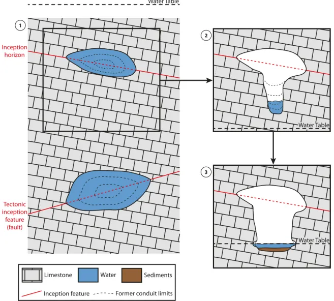
The dissolution process and the path development are not uniform in space due to the three-dimensional nature of the genesis processes and the geometrical anisotropy of the incep-tion features. These features favour a differential dissoluincep-tion, leading to an elongation of the conduits along them – often with pronounced angles – and explaining their non-cylindrical appearance in cross-section (figure2). The resulting shapes are consequently more or less elliptical depending, for instance, on the dissolution capacity of the fluids or on the contrast in permeability or in carbonate content between the inception feature and the surrounding formations[Filipponi,2009].
According to various authors, the groundwater table has a major influence on conduit development[e.g.,Jameson,1985,
Ford and Williams,2007,Farrant and Smart,2011,Jaillet et al.,
2011]. In the phreatic zone, corresponding to the saturated
zone below the water table, the inception features are the most influential factor upon the resulting shapes[Filipponi et al.,
2009]. The dissolution acts on whole conduits and in all
di-rections. The shapes are then more or less jagged, depending on the fluids, on the surrounding rocks and on the presence of other inception features (figure2,4.1)[e.g.,Jameson,1985,
Lauritzen and Lundberg,2000,Filipponi,2009]. The vadose
zone corresponds to the zone above the current water table. But the observed conduits are usually the result of a long pro-cess that has involved a past phreatic development. Keyhole passages are among the most common cross-sectional conduit geometries that are encountered[Field,2002]. They are
char-acterized by an entrenchment, a canyon passage commonly narrower than the original passage, also called the trench. In-deed, a drop of the water table puts the original conduits in phreatic conditions. The fluids circulating in the conduits with high velocities are led by gravity, incising the floor, generat-ing these typical cross-sectional keyhole shapes (figure3,4.2) [e.g.,Jameson,1985,Lauritzen and Lundberg,2000,Filipponi,
2009,Jaillet et al.,2011]. Horizontal dissolution notches are
less common. They develop at the water-table interface when conduits are partially flooded and water level variationsa are small enough to favour a lateral incision[e.g.,Lauritzen and Lundberg,2000,Ford and Williams,2007,Farrant and Smart,
2011]. Geometrically speaking, notches have a rounder aspect
than shapes linked to inception features (figure4.3).
In the following, we explain how these different observed geometries can be integrated in the ODSIM method to improve the realism of simulated karst conduits.
3 Principle of the object-distance
simula-tion method
Henrion et al.[2010] proposed an object-distance simulation
method (ODSIM) that models a three-dimensional envelope around a skeleton. For the explored parts of a karst, that skele-ton can be provided by field data, such as two-dimensional maps or LRUD (Left, Right, Up and Down) data. Otherwise,
Station n R L V D Station n+1 Conduit discretization Model Assembling
Figure 1 Classical conduit discretization process and 3D “reconstruction" used in common speleological programs (here with GHTopo).
Inception feature
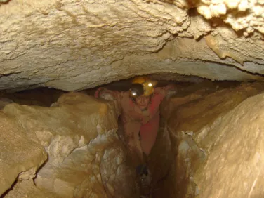
Figure 2 Examples of karstic conduits showing shapes strongly elongated along inception features (left: Cave O80, Switzerland; right: Grottes aux fées, Switzerland).
Figure 3 Example of a keyhole passage (Sieben Hengste Cave Sys-tem, Switzerland).
stochastic simulations can be used to obtain several skeletons and take into account the uncertainties related to the conduit location[e.g.,Pardo-Igúzquiza et al.,2011,Borghi et al.,2012,
Collon-Drouaillet et al.,2012]. The ODSIM method consists of
computing a Euclidean distance field around the skeleton and perturbing it using a random threshold (figure5). This thresh-old can be generated using a sequential Gaussian simulation (SGS) or other stochastic simulation methods[e.g.,Goovaerts,
1997,Deutsch and Journel,1997]. As a stochastic simulation
method, the SGS can provide an infinity of thresholds. This allows us to build several envelopes for a given skeleton, thus catching the uncertainties around the conduit shape. The per-turbation is done using the following indicator function:
IB(p) = ¨
1 if D(p) ≤ ϕ(p)
0 else (1)
D(p) is the 3D distance field computed at each point p = [px pypz]Tof a grid G andϕ(p) is the random threshold. The com-puted indicator property IB(p) is equal to 1 in the geological body, 0 outside. The 3D envelope corresponds to the surface at the interface between the interior and the exterior of the region corresponding to 1, or equivalently to points at a given distance of the network : D(p) ≤ ϕ(p). In this method, the simulated conduits can be complied with hard data condition-ing (like well data or LRUD distances to walls) thanks to an iterative Gibbs sampling algorithm[Geman and Geman,1984]
with inequality constraints[Freulon and de Fouquet,1993].
With this approach, the only way to avoid a globally cylindri-cal shape is to use plane skeletons instead of curves. However, the resulting envelope keeps a round aspect at the plane ex-tremities because of the Euclidean distance. Furthermore this approach lacks flexibility when dealing with various and com-plex shapes, such as those seen in section2.
4 Integration of geomorphological
infor-mation in ODSIM
The proposed methodology keeps the basic principle of ODSIM: the “distance” to an object model controls the first-order fea-tures while a random field provides the fine-scale feafea-tures [Henrion et al.,2010]. Our proposal is to play on these two
scales. First, by using a custom distance field generated by a fast marching method and constrained to geomorphological information. This allows us to take into account simultane-ously various elements involved in the conduit genesis and so influencing the conduit shapes. Second, we propose to build a random threshold by combining different variograms and/or distributions depending on the elements constraining the cus-tom distance field (figure6).
4.1 Using of a custom distance field instead of an
Euclidean distance field
The fast marching method[Sethian,1996,1999a,b] concerns
the propagation of a front knowing its speed. The principle is to solve the Eikonal equation:
|∇T |F = 1 (2)
Tis the time field and F the velocity field. 1/F gives a slowness field.
This method creates a scalar field corresponding to the ar-rival time T(x, y, z) at which the propagation front reaches the position(x, y, z), depending on a predetermined velocity field (or equivalently a slowness field) (figure7). This velocity field characterizes the speed of the front for each position(x, y, z). In a modelling approach, a convenient aspect is that the choice of the velocity field constrains the evolution of the front and the resulting arrival time field. Putting higher values for inception features in the velocity field constrains the time field in such a way that it contains geomorphological information, providing the custom distance field (figure7). Using a fast marching method gives thereby a greater flexibility to ODSIM. Nevertheless, the property used to compute the velocity field has to be thoughtfully chosen. As underlined byBorghi et al.
[2012], contrasts between the values are more important than
values themselves when using the fast marching method. The velocity field has to be linked with a property of the medium that respects this contrast rule.
As the notion of contrast controls both the fast marching and the karst genesis, the velocity field is built by using the permeability (or the hydraulic conductivity). This provides emphasis on the weakness planes, and moreover simplifies the choice of the property values. However, it is not sufficient to model specific structures like those encountered in the vadose zone and specific strategies need to be developed.
4.2 Building the velocity field for the vadose zone
Structures developed in vadose conditions are the result of several speleogenetic phases, corresponding to several water table positions. The goal of our method is not to reproduce each of these phases one after the other as a genetic model would do it. Instead, we propose numerical strategies to re-produce directly final conduit geometries consistent with the speleologist’s observations and knowledge.For reproducing the keyhole geometry, and more specifically the trenches appearing on the conduit floors, we propose to use an “attraction level" with high velocity values similar to those of the inception features. This attraction level may corre-spond to the present water table. A vertical plane between the skeleton and the attraction level is then considered as a high velocity zone by extending the attraction level values (figure
8). This modification constrains the front propagation which goes toward that level.
Water Table
Water Table
Water Table
Limestone Water
Inception feature Former conduit limits Inception horizon Tectonic inception feature (fault)
Phreatic development Vadose development
2
3 1
Sediments
Figure 4 Evolution of a karstic conduit depending on its position relative to the water table: 1. Genesis and growth of two conduits in the phreatic zone following different weakness planes (a lithostratigraphic horizon for the upper one, a fault for the other). 2. Following a fall of the water table, the upper conduit goes through the vadose zone which progressively generates a keyhole passage by cutting a trench. 3. Following a rise of the water table, notches grow at the trench bottom.
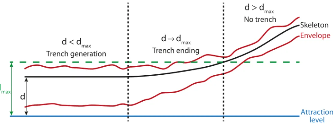
To limit the effects of the attraction level on the highest con-duits, a parameter representing the maximum allowed distance
dma xbetween the skeleton and the attraction level is added to generate these trenches. Moreover, the distance between the skeleton and the attraction level d is used to obtain shorter depths for trenches as the conduits move away from the wa-ter table. To do that, the permeability values of the attraction level in the vertical plane building the trenches are multiplied by a factor integrating d/dma x, giving the vertical trench plane velocity values v:
v(xs, ys, z) = m × (1 −
d(xs, ys)
dma x ) × pw(xs, ys, zw) (3)
(xs, ys, zs) is a point of the skeleton, (xw, yw, zw) is a point of the attraction level, z is bounded by zsand zw, m is a multiplication factor defined by the user, dma x sizes the zone of influence of the attraction level, v is the velocity value of the vertical plane at a given point(xs, ys, z), d is the distance between the skeleton and the attraction level at the same horizontal coordinates(xs, ys) and pw is the permeability value at the attraction level at the same horizontal coordinates(xs, ys).
Using d causes trench depth to evolve smoothly with the dis-tance between the skeleton and the attraction level and avoids sharp entrenchment endings on the boundaries of the influence zone (figure9). If the difference between the velocity values of the attraction level and those of the surrounding formation is not significant, the factor(1−d/dma x) can invert their contrast, leading to lower velocity values for the vertical plane and so a poor front propagation. The multiplication factor m solves this issue and gives the user a control on the trench depth.
With only one column of cells representing the vertical trench plane in the grid, the resulting trenches are V-shaped and do not show vertical sides or a flat bottom. Thus, several parame-ters are added to give more control to the propagation of the front and be sure it gives a satisfying shape to the envelope. The main point is to extend the vertical plane sideways, using a width w and a “beginning distance" db to ensure straighter sides of the trenches (figure10.1).
Notches are often smooth shapes created while the water table is superimposed on the conduits. These features can be easily modelled by thickening the (paleo)water table(s) in the velocity field using a factor n (figure 10.2). The thickening
X Y
Z
Skeleton Object
Distance Field D(p) Random Threshold φ(p)
Distance Field Truncation 1 if D(p) ≤ φ(p) 0 if not IB(p) = Geological Body IB(p)
Prior Geological Knowledge Hard and Soft Data
Sequential Gaussian Simulation 10 25 0 1 0 100 X Y Z X Y Z X Y Z X Y Z
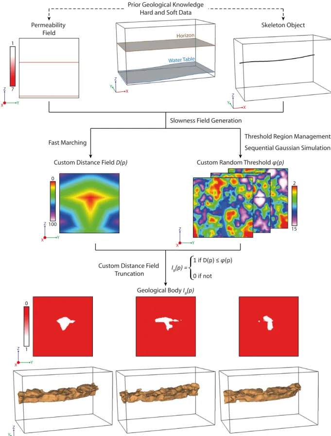
Figure 5 ODSIM workflow (modified fromHenrion et al.[2010]) applicated to a karstic conduit generation. The distance field D(p) is truncated with the random thresholdϕ(p) giving an indicator property IB(p) of the karstic conduits and caves.
controls the smoothness and the height of the notch shape. The notch depth can be controlled by applying a multiplication factor on the velocity values around the (paleo)water table(s).
4.3 Management of the different scales of
pertur-bations on the envelope
As said before, the velocity field controls the coarse-scale shape of the conduits, but the focus of the ODSIM approach is to combine this field with a random threshold that perturbs this “perfect" geometry by introducing fine-scale variability and also
allows hard data conditioning. In their paper,Henrion et al.
[2010] have proposed to introduce a locally variable mean into
the sequential Gaussian simulation in order to accommodate a spatial trend. But this kind of modification would equally affect roof, walls and floors of the conduits by a progressive growing or narrowing.
Considering cave conduit geometries, it appears that these fine-scale variabilities are not identically affecting the roof, the walls or the floor. Due to many different factors, like breaking-down, mechanical and chemical erosion, it is common to have more variabilities along a roof than, particularly, on the bottom
1
7
Permeability Field
Custom Distance Field D(p) Custom Random Threshold φ(p)
Custom Distance Field Truncation
1 if D(p) ≤ φ(p) 0 if not
IB(p) =
Geological Body IB(p)
Prior Geological Knowledge Hard and Soft Data
Threshold Region Management Sequential Gaussian Simulation Fast Marching 0 1 0 100 Y Z X 2 15 X Y Z Skeleton Object X Y Z Y Z X Y Z X
Slowness Field Generation X Y Z Horizon Water Table Y Z X
Figure 6 New workflow for ODSIM. The original method is obtained by using a constant velocity or slowness field and the same parameters for the whole threshold. Slowness field generation and fast marching steps are further detailed in sections4.1and4.2, threshold region management step is detailed in section4.3.
0 200 1 7 Velocity field Time field 0 90
Euclidean distance field
Figure 7 Comparison between an Euclidean distance field and a field generated by fast marching. Both fields are generated from the central node of the grid, but the time field is constrained by the differences of speed given by the velocity field.
Skeleton
Attraction level
Extension of the attraction level values
Figure 8 Foundations for trench modelling: a vertical plane between the skeleton and the attraction level is considered. The values of the attraction level crossed by the plane are extended vertically up to the skeleton.
dmax d d < dmax Trench generation d dmax Trench ending d > dmax No trench Skeleton Envelope Attraction level
Figure 9 Consequences on the envelope of the variations of the distance d between the skeleton and the attraction level, illustrating the impact of the formula (3). The permeability values pware taken from the attraction level and the distance dma x is defined by the user and
Fast Marching Fast Marching Slowness field Generation 0 40 0 40 0 1 Attraction level Horizon Skeleton Skeleton (paleo)water table Trench generation Notch generation db w n
db distance of beginning for the enlargement w number of cells on both sides of the vertical trench plane
n number of cells on both sides of the (paleo)water level Slowness field Generation 1 2 0 1
Figure 10 Modifications of the slowness field allowing the generation of trenches and notches. The global shape of these elements is clearly visible in the field created by fast marching.
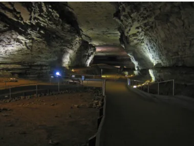
Figure 11 Example of a passage with different scales of perturba-tion: the top and the floor of the conduit are roughly flat whereas its sides are more wavy (Mammoth Cave, US).
of a trench. Thus, conduit irregularities are not symmetrical and, moreover, their variations do not range between the same extrema (figure11). Such differences between conduit ceiling, floor and/or sides can be noticed in several conduits, such as in the Abracurrie Main Chamber, Nullarbor, Australia[James et al.,2012] or in the Clearwater Cave, Gunung Mulu, Sarawak
[Farrant and Smart,2011].
To model a smooth trench floor, for instance, we propose to separate the grid in two areas: the first one contains the vertical trench planes – with eventually an extension around the planes to avoid trench side protuberances to develop below the trench floor when using very high perturbations, and the
second one the rest of the grid. Then two distinct variograms and/or distributions are defined in each area. The sequential Gaussian simulation generating the random threshold has to preserve a continuous resulting field between those areas (fig-ure12).
Increasing the range of the variogram used on the trench planes smoothes their bottom while preserving small scale per-turbation on the trench sides. Reducing the amplitude of the values used for the probability density function (PDF) on the trench planes avoids obtaining a large range of variation for the conduits at the bottom (figure13). The same method can be applied to reduce the roughness along weakness planes. Even-tually, the use of several variograms models and/or distribu-tions for each element controlling the shape gives differential perturbations of the envelope.
5 Results and discussion
These extensions of ODSIM have been implemented as a plu-gin of the GOCAD geomodelling software4and written in C++. It should be noted that this work can be developed in an other modelling software, in a numerical computing environment such as Matlab or Scilab as well as in a stand-alone application. The methodology has been tested on two synthetic cases. By using synthetic cases, we can easily demonstrate the new possi-bilities (cylinder, lens, keyholes, ...) offered by the method in a few examples, without falling into a controversial context. To better illustrate the independence between the skeleton simu-lation and the three-dimensional envelop modelling, the same karstic skeleton is used in the following examples. Inception features, water table and attraction level are modelled with
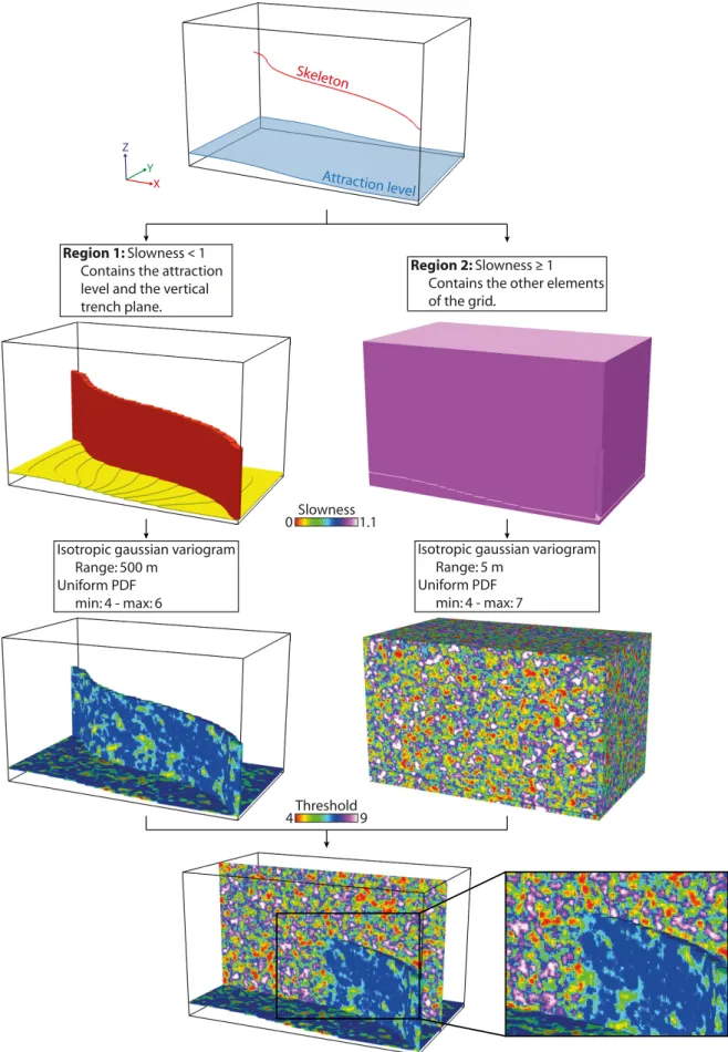
Isotropic gaussian variogram Range: 5 m
Uniform PDF min: 4 - max: 7 Isotropic gaussian variogram
Range: 500 m Uniform PDF min: 4 - max: 6 0Slowness1.1 4Threshold9 Region 1: Slowness < 1
Contains the attraction level and the vertical trench plane.
Region 2: Slowness ≥ 1 Contains the other elements of the grid. Attraction level Skeleton X Y Z
Figure 12 Threshold generation example: the principle is to separate the structures with different perturbation types using their values in the slowness field. Here only two areas are created: the last screenshot shows the region 1 together with a section along the whole x axis, showing elements of the region 2. The enlargement on the right shows the continuity between the features of the two areas despite the two different distributions and variograms. This continuity is essential for obtaining good quality envelopes.
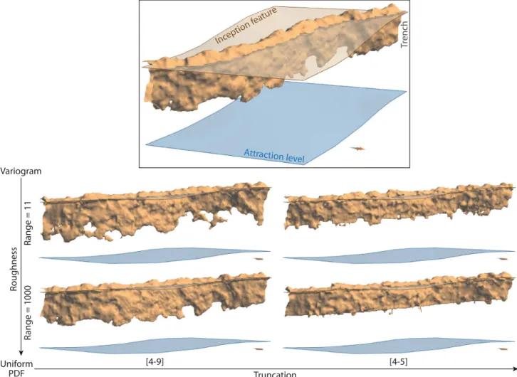
[4-9] [4-5] R ange = 11 R ange = 1000 Variogram Uniform PDF R oughness Truncation Attraction level Inception f eature Tr ench
Figure 13 Impact of the variogram and distribution used to generate the threshold: side view of the resulting envelopes. The given parameters are those of the weakness planes and the trench plane, the rest of the grid having a variogram range of 11 m and a uniform PDF of[4-9]. The velocity field values are 5 for the previous planes and 1 in the rest of the grid.
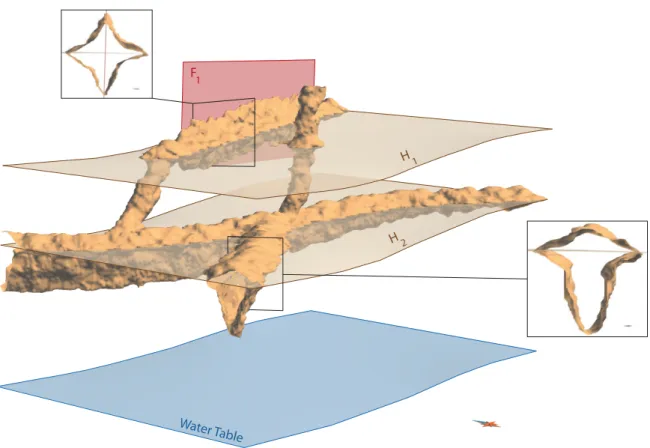
triangulated surfaces. For the threshold simulations, a regular structural grid has been used. Both examples are supposed to be the expression of two genetic phases: i) an initial phreatic phase that is visible on the final shapes through an elongation along inception features ; ii) and a second phase that results from a lowering of the water table. In the first example, to illustrate trench modelling capacities, an attraction level has been introduced at the water table level. The distance dma x has been chosen to limit entrenchments to the lowest conduit (figure14). The various parameters used in this simulation are presented in table1(Example 1). In the second example, we wanted to test the capacity of the method to reproduce notches (figure15). A water table is thus introduced at the same altitude as the lowest conduits. It is duplicated into an attraction level to simultaneously develop trenches on the up-per conduit, suup-perposed to the inception elongation features. Detailed parameters are presented in table1(Example 2).
The resulting envelopes reflect the various coarse-scale kars-tic shapes that are now possible to model with this new method-ology: i) lengthening and sharp incision along inception fea-tures (stratigraphical and tectonic) ; ii) realistic symmetric round shapes for the vertical conduits ; iii) trenches super-posed on a cylindrical or lens shape for keyhole passages ; iv) longitudinal notches. All these features can be combined. What trenches concern, depth variations follow the position of the conduits relatively to the attraction level: the further from the attraction level the conduits are, the lower is the trench
depth. Their bottom is smoother than the shapes linked to the inception features thanks to the combined use of different var-iograms and distributions in the random threshold generation. Notch representations are more like a rounding of the lateral carving although they can be more “marked" in the caves. The result remains useful in representing large notches. Generally, the proposed methodology offers an interesting list of solutions to simulate or reconstruct realistic three-dimensional karstic conduits. In this dual-scale geostatistical simulation method, the coarse-scale features can be modelled by an adapted and modular combination of a skeleton representation of the stud-ied object and geological/speleological constraints defined by the user. This results in a custom velocity field representing the coarse-scale geometries. A solution is proposed for man-aging the different fine-scale features depending on the same geological/speleological constraints. The Gibbs sampler with inequality constraints algorithm – which is already available in the method[Henrion et al.,2010] – complements this
tool-box by allowing hard data conditioning. Some further work is required to quantitatively validate the method capacity to re-produce realistic shapes. Several solutions could be explored: • Compare a cave already modelled using a LiDAR survey or 2D sections and maps with several simulated con-duits. Due to the stochastic nature of the process, the direct assessment of the real and simulated passage fit is worthless: a simulated conduit can be geomorpholog-ically consistent even if it does not fit the real conduit.
F
Water Table 1
H2
H1
Figure 14 Simulated envelope obtained by using two stratigraphic inception features (H1and H2), one tectonic inception feature (fault F1)
and an attraction level. Complex three-dimensional karst features such as trenches or elongated shapes are successfully reproduced.
F
1
Water Table
H1
Figure 15 Simulated envelope obtained by using one stratigraphic inception feature (H1), one tectonic inception feature (fault F1) and an
attraction level superimposed on a water table at the same level as the lowest conduits. Complex three-dimensional karst features such as notches, trenches or elongated shapes are successfully reproduced.
Table 1 Summary of parameters used to create the two synthetic models.
Example 1 Example 2
Grid parameters
Grid size (in cell) 250× 150 × 150 250× 150 × 150
Cell size (in m) 1× 1 × 1 1× 1 × 1
Fast marching parameters
Initial slowness field
H1slowness value 0.2 0.2
H2slowness value 0.2
-F1slowness value 0.2 0.2
Water table slowness value 0.2 0.2
Matrix slowness value 1 1
Trench parameters dma x(in m) 70 70 db(in cell) 4 4 w (in cell) 1 1 Notch parameters n (in cell) - 1 Threshold parameters
Low slowness region(Slowness < 1)
Variogram
Type Gaussian Gaussian
Range (in m) 500 500
Distribution
Type Uniform Uniform
Min - Max 4 - 6 4 - 6
High slowness region(Slowness = 1)
Variogram
Type Gaussian Gaussian
Range (in m) 7 7
Distribution
Type Uniform Uniform
Min - Max 4 - 7 4 - 7
Some indicators have to be developed to capture the en-tire three-dimensional characteristics of a conduit, such as, for instance, the conduit volume or the ratio of con-duit surface area to concon-duit volume. Those indicators are then used to compare the real conduit and the sim-ulated ones.
• Compare the simulated shapes for the unknown parts of a network with the conditioned shapes in the known parts based on statistical or fractal-based principles such as introduced byCurl[1986] [e.g.,Pardo-Igúzquiza et al.,
2011].
Despite these encouraging results, some limitations appear. First, the grid resolution can have a significant impact on the results. Indeed the introduction of the inception features in a velocity property corresponds to their rasterization in the grid. Stratigraphic inception horizons have a thickness of some cen-timetres to some decimetres[Filipponi,2009], and conduits
may be very stretched along them. Moreover, tectonic incep-tion features induce very thin shapes at the intersecincep-tion with the conduit. This means that shape modelling requires high grid resolutions, at least to represent the global shape of the
0 90
Figure 16 Insufficient grid resolution leading to a non-continuous karstic conduit simulation. The colours correspond to the custom distance field and the transparent surface represents the weakness plane.
conduits in an acceptable way (figure16). Another solution would be to have a non-regular grid organized along inception features. Second, the increase of the degrees of freedom in the process has a direct consequence on the increase of user choices and parameters, even if many features can be inte-grated directly in the custom distance field. But this last limi-tation is directly linked to the complexity of the studied case and difficult to avoid. Nevertheless, perhaps a new alternative could be found that avoids the use of the dband w parameters in the trench modelling process.
As for perspectives, a modelling method for other shapes could be studied. For instance paragenetic caves are made of conduits developed in the phreatic zone shaped like upside-down trenches, displaying an upward entrenchment of con-duits (figure17)[Renault,1958, 1968,Pasini,1967]. They
could probably be modelled with the same principle as trenches, but upturned. Another common geometry, partially linked to breakdowns, is strike-oriented passages[e.g.,Palmer,2012]
that have a polygonal shape following horizons, with many perpendicular angles (figure18). Even if various scales of vari-ability are introduced in the simulated conduits through the threshold field, small-scale features such as scallops can still not be clearly and deliberately represented. On the other hand, larger scale features, such as conduit loops, are not linked to the conduit shape but to the network and should be introduced by the skeleton.
In a broader perspective, tests are required to assess the impact of these shapes on flow simulations . Modelling sed-iments could also be interesting considering their impact on fluid flows and on speleogenesis[Farrant and Smart,2011].
Finally, the entire methodology could be adapted to other un-derground processes, such as hydrothermal alteration, or be used to study the usefulness and applicability of the method in sinkhole prevention.
Conclusions
These improvements of ODSIM allow the stochastic genera-tion of karst conduit envelopes around a skeleton by taking
Limestone Water
Inception horizon Former sediments limits Sediments
Water Table
Figure 17 Principle of the development of the paragenetic conduits: sediments progressively fill the cavity and block the downward dissolution, which favours an upward dissolution propagation.
Limestone
Figure 18 A strike-oriented passage: the conduit shape follows lithostratigraphic horizons.
into account local geological information, especially inception features and (paleo)water table. It consequently contributes to the global workflow of stochastic karst generation, comple-menting the methods that stochastically generate skeletons rep-resenting the general network by introducing geomorphologi-cally consistent conduit shapes. Various classic conduit shapes can be simulated, such as elongated or keyhole passages, while preserving the original capacities of ODSIM. Some other par-ticular shapes still need to be taken into account to allow their simulation. Applying this method on synthetic cases gives quite satisfying results. The simulated shapes finely reproduce the most common conduit geometries while controlling the dif-ferent scales and areas of shape perturbations. However, a confrontation to real data still needs to be carried out; first to validate the application to the reconstruction of explored and monitored conduits, then to validate more objectively the method’s capacity to generate realistic conduits.
Acknowledgements
We would like to thank the industrial and academic members of the Gocad Consortium5, especially Paradigm for providing
5http://www.gocad.org
the Gocad Software and API, ASGA (Association Scientifique pour la Géologie et ses Applications) and the French National Scientific Research Center CNRS-GeoRessources for their sup-port. We would also like to thank the reviewers, including Ph. Häuselmann, for constructive comments which helped im-prove this paper. This work was performed in the framework of the “Investissements d’avenir” Labex RESSOURCES21 (ANR-10-LABX-21).
References
M. Boggus and R. Crawfis. Explicit generation of 3D models of solution caves for virtual environments. In Proceedings of the 2009 International
Conference on Computer Graphics and Virtual Reality, pages 85–90, 2009.
(Cited page2)
A. Borghi, P. Renard, and S. Jenni. A pseudo-genetic stochastic model to generate karstic networks. Journal of Hydrology, 414-415:516–529, 2012.
(Cited pages1and4)
R. Brinkmann, M. Parise, and D. Dye. Sinkhole distribution in a rapidly developing urban environment: Hillsborough County, Tampa Bay area, Florida. Engineering Geology, 99(3-4):169–184, 2008. (Cited page1)
Z. Chaojun, J. Chengzao, L. Benliang, L. Xiuyu, and L. Yunxiang. Ancient karsts and hydrocarbon accumulation in the middle and western parts of the North Tarim uplift, NW China. Petroleum Exploration and Development, 37(3):263–269, 2010. (Cited page1)
P. Collon-Drouaillet, V. Henrion, and J. Pellerin. An algorithm for 3D simulation of branchwork karst networks using Horton parameters and A-star. applica-tion to a synthetic case. Geological Society of London - Special Publicaapplica-tions, 370(1):12, 2012. doi: 10.1144/SP370.3. (Cited pages1and4)
R. L. Curl. Fractal dimensions and geometries of caves. Mathematical Geology, 18(8):765–783, 1986. (Cited page13)
J. De Waele, L. Plan, and P. Audra. Recent developments in surface and subsurface karst geomorphology: An introduction. Geomorphology, 106 (1-2):1–8, 2009. ISSN 0169-555X. doi: 10.1016/j.geomorph.2008.09.023.
(Cited page1)
J. De Waele, F. Gutiérrez, M. Parise, and L. Plan. Geomorphology and nat-ural hazards in karst areas: A review. Geomorphology, 134:1–8, 2011.
(Cited page1)
C. V. Deutsch and A. G. Journel. GSLIB: Geostatistical Software Library and
User’s Guide (Applied Geostatistics). Oxford University Press, USA, 1997.
(Cited page4)
A. R. Farrant and P. L. Smart. Role of sediment in speleogenesis; sed-imentation and paragenesis. Geomorphology, 134(1-2):79 – 93, 2011.
(Cited pages2,9, and13)
T. Faulkner. Tectonic inception in Caledonide marbles. Acta Carsologica, 35 (1):7–21, 2006. (Cited page2)
M. S. Field. A lexicon of cave and karst terminology with special reference to
envi-ronmental karst hydrology. National Center for Environmental Assessment -Washington Office, Office of Research and Development, US Environmental Protection Agency, 2002. (Cited page2)
M. S. Field and P. F. Pinsky. A two-region nonequilibrium model for solute transport in solution conduits in karstic aquifers. Journal of Contaminant
Hydrology, 44:329–351, 2000. (Cited page1)
M. Filipponi. Spatial Analysis of Karst Conduit Networks and Determination of
Parameters Controlling the Speleogenesis along Preferential Lithostratigraphic Horizons. PhD thesis, École Polytechnique Fédérale de Lausanne, Suisse, 2009. (Cited pages2and13)
M. Filipponi, P.-Y. Jeannin, and L. Tacher. Evidence of inception hori-zons in karst conduit networks. Geomorphology, 106(1):86–99, 2009.
(Cited page2)
M. Filipponi, P.-Y. Jeannin, and L. Tacher. Understanding cave genesis along favourable bedding planes. the role of the primary rock permeabil-ity. Zeitschrift für Geomorphologie, Supplementbände, 54(2):91–114, 2010.
(Cited page2)
D. Ford and P. Williams. Karst Hydrogeology and Geomorphology. John Wiley and Sons, Ltd., 2007. ISBN 978-0-470-84996-5. (Cited pages1and2)
X. Freulon and C. de Fouquet. Conditioning a gaussian model with inequali-ties. In A. Soares, editor, Geostatistics Tróia ’92, number 5 in Quantitative Geology and Geostatistics, pages 201–212. Springer Netherlands, 1993.
(Cited page4)
A. Frumkin, P. Karkanas, M. Bar-Matthews, R. Barkai, A. Gopher, R. Shahack-Gross, and A. Vaks. Gravitational deformations and fillings of aging caves: The example of Qesem karst system, Israel. Geomorphology, 106(1-2): 154–164, 2009. (Cited page1)
S. Geman and D. Geman. Stochastic relaxation, Gibbs distributions, and the Bayesian restoration of images. Pattern Analysis and Machine Intelligence,
IEEE Transactions on, (6):721–741, 1984. (Cited page4)
N. Goldscheider. A new quantitative interpretation of the long-tail and plateau-like breakthrough curves from tracer tests in the artesian karst aquifer of Stuttgart, Germany. Hydrogeology Journal, 16:1311–1317, 2008.
(Cited page1)
P. Goovaerts. Geostatistics for natural resources evaluation. Applied Geostatis-tics. Oxford University Press, New York, 1997. ISBN 0-19-511538-4. 483p.
(Cited page4)
A. Hartmann, J. Lange, A. V. Aguado, N. Mizyed, G. Smiatek, and H. Kunst-mann. A multi-model approach for improved simulations of future water availability at a large Eastern Mediterranean karst spring. Journal of
Hy-drology, 468-469:130–138, 2012. (Cited page1)
M. Hauns, P.-Y. Jeannin, and O. Atteia. Dispersion, retardation and scale effect in tracer breakthrough curves in karst conduits. Journal of Hydrology, 241: 177–193, 2001. (Cited page1)
V. Henrion, G. Caumon, and N. Cherpeau. ODSIM: An object-distance simu-lation method for conditioning complex natural structures. Mathematical
Geosciences, 42.8:911–924, 2010. (Cited pages2,4,6, and11)
N. Horvatinˇci´c, I. Krajcar Broni´c, and B. Obeli´c. Differences in the14C
age, δ13C andδ18O of Holocene tufa and speleothem in the Dinaric karst. Palaeogeography, Palaeoclimatology, Palaeoecology, 193:139–157, 2003. (Cited page1)
S. Jaillet, B. Sadier, J. Arnaud, M. Azéma, E. Boche, D. Cailhol, M. Filipponi, P. L. Roux, and E. Varrel. Topographie, représentation et analyse morphologique 3D de drains, de conduits et de parois du karst. Images et modèles 3D en
milieux naturels, pages 119–130, 2011. (Cited page2)
J. M. James, A. K. Contos, and C. M. Barnes. Nullarbor caves, Australia.
In: William B. White and David C. Culver (Editors), Encyclopedia of Caves, Second Edition, Elsevier Science, pages 568–576, 2012. (Cited page9)
R. A. Jameson. Structural segments and the analysis of flow paths in the North Canyon of Snedegar Cave, Friars Hole Cave System. Master’s thesis, West Virginia University, Morgantown, 1985. (Cited page2)
T.-S. Kuo, Z.-Q. Liu, H.-C. Li, N.-J. Wan, C.-C. Shen, and T.-L. Ku. Climate and environmental changes during the past millennium in central western Guizhou, China as recorded by Stalagmite ZJD-21. Journal of Asian Earth
Sciences, 40:1111–1120, 2011. (Cited page1)
R. Labourdette, I. Lascu, J. Mylroie, and M. Roth. Process-like modeling of flank-margin caves: from genesis to burial evolution. Journal of
Sedimen-tary Research, 77:965–979, 2007. (Cited page2)
S. E. Lauritzen and J. Lundberg. Solutional and erosional morphology.
Speleo-genesis: Evolution of Karst Aquifers: Huntsville, Ala., National Speleological Society, pages 408–426, 2000. (Cited page2)
D. J. Lowe. The origin of limestone caverns: An inception horizon hy-pothesis. PhD thesis, Manchester Polytechnic, United Kingdom, 1992.
(Cited page2)
X. Lü, N. Yang, X. Zhou, H. Yang, and J. Li. Influence of Ordovician carbonate reservoir beds in Tarim Basin by faulting. Science in China Series D: Earth
Sciences, 51:53–60, 2008. (Cited page1)
G. Mongelli. Growth of hematite and boehmite in concretions from an-cient karst bauxite: clue for past climate. Catena, 50:43–51, 2002.
(Cited page1)
T. Morales, J. A. Uriarte, M. Olazar, I. naki Antigüedad, and B. Angulo. Solute transport modelling in karst conduits with slow zones during dif-ferent hydrologic conditions. Journal of Hydrology, 390:182–189, 2010.
(Cited page1)
B. P. Onac and S. Constantin, editors. Archives of Climate and Environ-mental Change in Karst. Quaternary International, volume 187. 2008.
(Cited page1)
A. N. Palmer. Solution caves in regions of moderate relief. In: William B.
White and David C. Culver (Editors), Encyclopedia of Caves, Second Edition, Elsevier Science, pages 733–743, 2012. (Cited page13)
E. Pardo-Igúzquiza, J. J. Durán-Valsero, and V. Rodríguez-Galiano. Morpho-metric analysis of three-dimensional networks of karst conduits.
Geomor-phology, 132:17–28, 2011. (Cited pages4and13)
E. Pardo-Igúzquiza, P. A. Dowd, X. Chaoshui, and J. J. Durán-Valsero. Stochas-tic simulation of karst conduit networks. Advances in Water Resources, 35(0309-1708):ISI:000300031000012, 2012. doi: 10.1016/j.advwatres. 2011.09.014. (Cited page1)
M. Parise, J. De Waele, and F. Gutiérrez. Current perspectives on the envi-ronmental impacts and hazards in karst. Envienvi-ronmental Geology, 58(2): 235–237, 2009. (Cited page1)
G. Pasini. Nota preliminare sul ruolo speleogenetico dell’erosione “antigravi-tativa". Le Grotte d’Italia, 4(1):75–90, 1967. (Cited page13)
P. Renault. Eléments de spéléomorphologie karstique. Annales de Spéléologie, 13(1-4):23–48, 1958. (Cited page13)
P. Renault. Contribution à l’étude des actions mécaniques et sédimentologiques dans la spéléogenèse. 3e partie : Les facteurs sédimentologiques. Annales
de Spéléologie, 23(3):529–596, 1968. (Cited page13)
J. Sethian. A fast marching level set method for monotonically advancing fronts. Proceedings of the National Academy of Sciences, 93(4):1591–1595, 1996. (Cited page4)
J. Sethian. Fast marching methods. SIAM Review, 41(2):199–235, 1999a.
(Cited page4)
J. Sethian. Level set methods and fast marching method. In Cambridge
University Press, Cambridge, United Kingdom, 1999b. (Cited page4)
H. A. Viles. Conceptual modeling of the impacts of climate change on karst geomorphology in the UK and Ireland. Journal for Nature Conservation, 11: 59–66, 2003. (Cited page1)
![Figure 5 ODSIM workflow (modified from Henrion et al. [ 2010 ] ) applicated to a karstic conduit generation](https://thumb-eu.123doks.com/thumbv2/123doknet/14792765.602151/7.892.129.783.63.902/figure-workflow-modified-henrion-applicated-karstic-conduit-generation.webp)