Comparison of CO₂ fluxes estimated using atmospheric and oceanic inversions, and role of fluxes and their interannual variability in simulating atmospheric CO₂ concentrations

HAL Id: hal-00302003

https://hal.archives-ouvertes.fr/hal-00302003

HAL is a multi-disciplinary open access

archive for the deposit and dissemination of sci-entific research documents, whether they are pub-lished or not. The documents may come from teaching and research institutions in France or abroad, or from public or private research centers.

L’archive ouverte pluridisciplinaire HAL, est destinée au dépôt et à la diffusion de documents scientifiques de niveau recherche, publiés ou non, émanant des établissements d’enseignement et de recherche français ou étrangers, des laboratoires publics ou privés.

Comparison of CO2 fluxes estimated using atmospheric

and oceanic inversions, and role of fluxes and their

interannual variability in simulating atmospheric CO2

concentrations

P. K. Patra, S. E. Mikaloff Fletcher, K. Ishijima, S. Maksyutov, T. Nakazawa

To cite this version:

P. K. Patra, S. E. Mikaloff Fletcher, K. Ishijima, S. Maksyutov, T. Nakazawa. Comparison of CO2 fluxes estimated using atmospheric and oceanic inversions, and role of fluxes and their interannual variability in simulating atmospheric CO2 concentrations. Atmospheric Chemistry and Physics Dis-cussions, European Geosciences Union, 2006, 6 (4), pp.6801-6823. �hal-00302003�

ACPD

Full Screen / Esc

Printer-friendly Version Interactive Discussion Atmos. Chem. Phys. Discuss., 6, 6801–6823, 2006

www.atmos-chem-phys-discuss.net/6/6801/2006/ © Author(s) 2006. This work is licensed

under a Creative Commons License.

Atmospheric Chemistry and Physics Discussions

Comparison of CO

₂

fluxes estimated

using atmospheric and oceanic

inversions, and role of fluxes and their

interannual variability in simulating

atmospheric CO

₂

concentrations

P. K. Patra1, S. E. Mikaloff Fletcher2, K. Ishijima1, S. Maksyutov3, and T. Nakazawa4

1

Frontier Research Center for Global Change, Japan Agency for Marine-Earth Sciences and Tecnology, Yokohama 236 0001, Japan

2

Atmospheric and Oceanic Sciences, Princeton University, Sayre Hall, Forrestal Campus, P.O. Box CN0710, Princeton, NJ, 08544-0710, USA

3

Center for Global Environmental Research, National Institute for Environmental Studies, Tsukuba 305-8506, Japan

4

Center for Atmospheric and Oceanic Studies, Graduate School of Science, Tohoku University, Sendai 980-8578, Japan

Received: 5 May 2006 – Accepted: 7 July 2006 – Published: 20 July 2006 Correspondence to: P. K. Patra (prabir@jamstec.go.jp)

ACPD

Full Screen / Esc

Printer-friendly Version Interactive Discussion

Abstract

We use a time-dependent inverse (TDI) model to estimate regional sources and sinks of atmospheric CO₂from 64 and then 22 regions based on atmospheric CO₂ observa-tions at 87 staobserva-tions. The air-sea fluxes from the 64-region atmospheric-CO₂ inversion are compared with fluxes from an analogous ocean inversion that uses ocean interior

5

observations of dissolved inorganic carbon (DIC) and other tracers and an ocean gen-eral circulation model (OGCM). We find that, unlike previous atmospheric inversions, our flux estimates in the southern hemisphere are generally in good agreement with the results from the ocean inversion, which gives us added confidence in our flux es-timates. In addition, a forward tracer transport model (TTM) is used to simulate the

10

observed CO₂concentrations using (1) estimates of fossil fuel emissions and a priori estimates of the terrestrial and oceanic fluxes of CO₂, and (2) two sets of TDI model corrected fluxes. The TTM simulations of TDI model corrected fluxes show improve-ments in fitting the observed interannual variability in growth rates and seasonal cycles in atmospheric CO₂. Our analysis suggests that the use of interannually varying (IAV)

15

meteorology and a larger observational network have helped to capture the regional representation and interannual variabilities in CO₂fluxes realistically.

1 Introduction

Regular observations of atmospheric CO₂ concentrations in the troposphere indicate that its growth rate and seasonal cycle vary interannually (Bacastow, 1979; Conway

20

et al., 1994; Keeling et al., 1995; Langenfeld et al., 2002; Matsueda et al., 2002; Levin et al., 2003). The secular trends in CO₂concentrations and a major component of the interannual variations in the seasonal cycle and growth rates are caused by changes in the sources and sinks of CO₂ to the atmosphere due to increasing fossil fuel emissions (Marland et al., 2003), CO₂ fluxes due to land-use change (Houghton,

25

ACPD

Full Screen / Esc

Printer-friendly Version Interactive Discussion Jones and Cox, 2005; Patra et al., 2005). Thus, the interannual variability in regional

and global CO₂ fluxes are often estimated using time-dependent inverse modeling of atmospheric CO₂with the aid of a TTM (e.g. Rayner et al., 1999; Bousquet et al., 1999; R ¨odenbeck et al., 2003a, b; Patra et al., 2005a, b; Baker et al., 2006). The TTM is used to describe how fluxes from a given region influence the spatial and temporal pattern of

5

atmospheric CO₂based on fluxes at the earth’s surface and meteorological variables (winds, temperature, humidity etc.).

Efforts to validate the results obtained by atmospheric CO₂ inverse modeling and other estimates have been gaining interest recently (e.g. McKinley et al., 2004; Peylin et al., 2005; Patra et al., 2005b). These studies compared the anomalies in CO₂fluxes

10

with terrestrial and oceanic biogeochemical modeling results. In addition, extensive model comparison studies have been done to elucidate potential biases due to the choice of TTM in the inversion through the TransCom-3 model intercomparison project (e.g. Gurney et al., 2004; Baker et al., 2006). In the TransCom-3 experiments, up to 16 atmospheric transport models or model variants are used to quantify the errors in

15

estimated CO₂ fluxes arising from differences in model transport. However, not much has been done to use the inverse flux estimates to simulate the interannual variability, seasonal cycles, and growth rates of atmospheric CO₂ at the observing stations and quantify the improvements in the time-dependent flux estimates at regional scales. So far, quantitative validation of spatial distributions of CO₂ fluxes have been limited to

20

the oceanic regions (e.g., Patra et al., 2005a), because observing stations that sample land regions are often contaminated by local sources that are not well represented in the models (Patra et al., 2006).

The aim of this study is to validate the results of the atmospheric inversion of Patra et al. (2005a, b) using two different approaches. First, we compare the

atmospheric-25

CO₂inversion results (Patra et al., 2005a) with those obtained from an ocean inversion that employs both different observations and different models (Mikaloff Fletcher et al., 2006a, b1). Unlike atmospheric inversions, the ocean inversion is not believed to be

1

Mikaloff Fletcher, S. E., Gruber, N., Jacobson, A. R., Doney, S. C., Dutkiewicz, S., Gerber,

ACPD

Full Screen / Esc

Printer-friendly Version Interactive Discussion data limited due to the greater spatial density of the data. Furthermore, the spatial

patterns associated with air-sea fluxes are well preserved in the ocean as a result of the long time scale of ocean circulation (Gloor et al., 2003; Mikaloff Fletcher et al., 2006a, b1). We compare these flux estimates from the ocean inversion with the 1988–2000 mean of the atmospheric inverse estimates, since the ocean inversion has only been

5

used to estimate the long term mean air-sea fluxes. We also examine the impact of the measurement network by comparing the long term mean results based on several different subsets of the 87 station measurement network.

Secondly, we analyze the effect of using IAV meteorology in the TTM on the flux vari-ability for specific regions and identify the areas that are most sensitive to changes in

10

meteorology due to the dominant climate oscillations. The TDI model corrected fluxes are used for TTM simulations, and quantitative estimates of the fit between model sim-ulations and observations are made for the year-to-year variations in seasonal cycles and growth rates of atmospheric CO₂. It may seem trivial to assume that TDI derived fluxes will automatically fit the observations well, because these measurements have

15

been used as constraints in the inversion. Nevertheless, if the global total or distribu-tion of regional fluxes are not derived properly due to errors in TDI model setup, the spatial pattern, inter-annual variability and long-term trends of the observations would not be simulated well by the TTMs. Therefore, this is an essential test of the inverse model results.

20

2 Materials and methods

The 64- and 22-region time-dependent inverse models are used to derive the monthly-mean CO₂ fluxes for the period January 1988–December 2001 (Patra et al., 2005a, b). Both the TDI models are based on Rayner et al. (1999) and follow the TransCom-3

M., Follows, M., Joos, J., Lindsay, K., Menemenlis, D., Mouchet, A., M ¨uller S. A., and Sarmiento,

J. L.: Inverse Estimates of preindustrial CO₂ fluxes, Global Biogeochem. Cycles, submitted,

ACPD

Full Screen / Esc

Printer-friendly Version Interactive Discussion protocol for the background fluxes and the spatial and seasonal source distributions

within the regions (Gurney et al., 2004). However, the 64-region TDI model (TDI/64) has more degrees of freedom for flux optimisation (larger number of regions) compared to TransCom-3, and this inverse model setup uses IAV meteorology and CO₂ obser-vations at a maximum of 87 stations. In this study, three configurations of the TDI/64

5

model are employed: 1. fully IAV meteorology (TDI/64-IAV), 2. year 1997 meteorol-ogy in cyclic mode (i.e., cyclostationary), the later half-year representing the dynamical conditions corresponding to an El Ni ˜no (TDI/64-1997), and 3. cyclostationary meteo-rology for the year 2000 (TDI/64-2000). The year 2000 meteometeo-rology is not substantially impacted by the El Ni ˜no Southern Oscillation (ENSO) cycle (Walker, 1910), but is

mod-10

erately influenced by the positive North Atlantic Oscillation (NAO) (Hurrel et al., 2003). These dynamical sensitivity runs are used to assess the possible benefits of IAV mete-orology in deriving interannual variability in CO₂fluxes at regional scales with respect to the cyclostationary meteorology. We also employed a variety of different network configurations in order to elucidate the effect of network selection on the inverse flux

15

estimates. The framework of the 22-region TDI model (TDI/22-IAV; ref. Fig.1 for the region divisions) is similar to that in Baker et al. (2006), but uses IAV meteorology. The inversions for regional CO₂ fluxes using atmospheric-CO₂ data will be referred to as ATMOS-INV.

The ocean inversion was developed by Gloor et al. (2001). It analogous to

ATMOS-20

INV, but it is completely independent from this method because it employs Ocean Gen-eral Circulation Models (OGCMs) rather than TTMs and is constrained by ocean interior observations rather than atmospheric observations. This method is described in Gloor et al. (2001, 2003), Jacobson et al. (2006)2, and Mikaloff Fletcher et al. (2006a, b1). The ocean inversion is not believed to be data limited due to the large number of

obser-25

vations and the footprint of air-sea flux being well preserved in the interior ocean. The

2 _{Jacobson, A. R., Mikaloff Fletcher, S. E., Gruber, N., Sarmiento, J. L., Gloor, M., and}

TransCom Modelers: A joint atmosphere-ocean inversion for surface fluxes of carbon dioxide: I. Methods and Global-Scale Fluxes, Global Biogeochem. Cycles, submitted, 2006.

ACPD

Full Screen / Esc

Printer-friendly Version Interactive Discussion air-sea fluxes estimated by the ocean inversion differ substantially from TransCom-3,

particularly in the tropics and temperate southern hemisphere, which has profound im-plications for the land fluxes (Jacobson et al., 20062). The ocean inversion estimates separately preindustrial (Mikaloff Fletcher et al., 2006b1) and anthropogenic (Mikaloff Fletcher et al., 2006a) fluxes from 30 geographic regions. In order to compare with

5

these estimates, we sum the anthropogenic and preindustrial components and aggre-gate to 11 ocean regions as labeled in Fig.1. Finally, we add an estimate of fluxes due to riverine carbon following Jacobson et al. (2006)2.

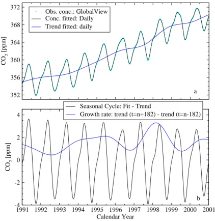
The weekly and daily mean observed or simulated CO₂concentrations are fitted by a digital filter to derive the best fit curve and a slowly varying long-term trend component

10

in the timeseries (Fig.2a). We used the filtering method of Nakazawa et al. (1997). The order of Butterworth filter is set to 26 for long-term trends. The growth rates discussed here are calculated as the differences in long-term trend values 365 days apart; e.g., the growth rate on 2 July 1995 is the difference in values between 1 January 1995 and 31 December 1995. The long-term trend values are subtracted from the best fit

15

curve to calculate the seasonal cycles (Fig.2b). The GlobalView data product, which is based on measurements from several international laboratories, was used to represent the weekly atmospheric CO₂ concentrations in this study (GlobalView-CO2, 2005). GlobalView is based on regular samples collected at a globally distributed network of observing stations, which are then adjusted to a single scale in order to account for

20

differences in individual laboratories’ standard scales. In order to create a consistent time series, these observations are fit to a smoothed curve, which is then sampled at regular 7.6 day intervals. In cases where the data record is incomplete, the existing observations are extended based on observations at similar latitudes (Masarie and Tans, 1995).

25

The NIES/FRCGC tracer transport model is used to simulate CO₂ concentrations globally at a 2.5×2.5 horizontal grid and 15 vertical layers in the troposphere (Maksyu-tov and Inoue, 2000). The known distributions for fossil fuel emission, terrestrial bio-spheric flux and ocean exchange or prior fluxes in the TDI models, and TDI model

ACPD

Full Screen / Esc

Printer-friendly Version Interactive Discussion corrected emissions are used for transport model simulations. The TDI model

esti-mated monthly flux corrections are distributed within the inverse model regions as per the basis function maps. In brief, the ocean basis functions have a uniform spatial distri-bution within each TDI model region except for a seasonally varying sea ice mask, and the spatial distribution within each land region follows the annual mean distribution of

5

net primary productivity from the CASA terrestrial biosphere model (Randerson et al., 1997). Three cases of transport model simulations are conducted using: 1. TDI/64-IAV corrected fluxes, 2. TDI/22-IAV corrected fluxes, and 3. TDI/64-IAV corrected fluxes, but with faster vertical diffusion (TDI/64-FD). For the latter simulation, the minimum verti-cal diffusion coefficient is increased to 120 m2s−1, which is otherwise set at 40 m2s−1.

10

The increased vertical diffusion is used to quantify the role this transport component in simulating atmospheric-CO₂concentrations.

3 Results and discussion

3.1 Comparison of regional flux estimations

We show the long-term averages of regional flux estimates from OCN-INV (Mikaloff

15

Fletcher et al., 2006a) and the TDI/64 model results obtained using several observation networks (Table1) and by various groups (Fig.3). As stated earlier, the ocean inver-sion estimates sea-air fluxes with an unprecedented accuracy (see column 3, Table1), and we treat this estimate as the yardstick for evaluating flux estimates by ATMOS-INV. Nevertheless, the ocean inversion has its own limitations and sources of uncertainty,

20

which are discussed extensively by Mikaloff Fletcher et al. (2006a, b1). Our compar-ison suggests that, overall, the fluxes using atmospheric-CO₂ at 87-stations (Patra et al., 2005a) are closest to the ocean inversion results. The largest discrepancies are found for the North Pacific, Northern Ocean, South Atlantic. However, the absolute differences in the two sets of flux estimates are only about 0.2 Pg-C yr−1. Other recent

25

studies using ATMOS-INV produced fairly similar sea-air CO₂fluxes at the hemispheric 6807

ACPD

Full Screen / Esc

Printer-friendly Version Interactive Discussion spatial scales when averaged over the 1990’s (not shown) (R ¨odenbeck et al., 2003;

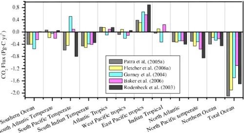
Patra et al., 2005; Baker et al., 2006). The global oceanic uptake estimate generally ranges between 1.0 and 2.1 Pg-C yr−1 in these studies. There are also considerable differences between the estimates at ocean basin scales (ref. Fig.3). The sum of vari-ances between OCN-INV and all other ATMOS-INV are about 0.26, 0.46, 0.96 and 1.44

5

(Pg-C yr−1)2for Patra et al. (2005a); Baker et al. (2006); R ¨odenbeck et al. (2003), and Gurney et al. (2004). We must clarify here that the estimates of Gurney et al. (2004) are based on cyclostationary inversion corresponding to the period 1992–1996, and may not represent the long-term mean flux (TransCom-3, seasonal flux estimate). Baker et al. (2006) fluxes are derived using similar inversion technique that used 13 different

10

atmospheric transport models (TransCom-3, IAV flux estimate), but this study does not take into account IAV in meteorology. The inversion approach adopted in R ¨odenbeck et al. (2003) is unique and has the highest in spatial resolution among the ATMOS-INV models described here. These authors used CO₂observations at 35 sites.

The agreement between atmospheric and ocean inversion fluxes is not as

satisfac-15

tory when smaller observing networks are used in the atmospheric inversion, and large differences can be found for more than one regions (Table 1). For most regions, we also obtained significant reduction, up to 50%, in flux uncertainties by the using the largest atmospheric-CO₂ observation network (Patra et al., 2005a) compared to the estimations using 19-stations network. There are also large changes in flux estimates

20

between these two networks. For example, the North Pacific and Southern Ocean be-come a weaker sink and stronger sink, respectively, when the larger network is used. For the intermediate size station networks (67 and 75 stations), the largest difference is found for the South Pacific flux. This is due to the use of CO₂ data from Easter Island (EIC) station. A sensitivity run of TDI model without the EIC station produces

25

fluxes −0.24, 0.25, and 0.35 Pg-C yr−1 for Tropical West and East Pacific, and South Pacific regions, respectively. Thus, by using the EIC station data in inversion, a closer agreement in the spatial distribution of fluxes for the entire tropical and south Pacific Ocean basin is obtained between OCN-INV and ATMOS-INV (column 1 and 2 in

Ta-ACPD

Full Screen / Esc

Printer-friendly Version Interactive Discussion ble1, respectively). Since the 87-station network has the highest spatial coverage of

CO₂ measurements and the derived fluxes compare well with those using OCN-INV, we shall utilise the results based on this network in the remaining part of the discussion. 3.2 Effect of TTM meteorology on TDI derived interannual CO₂flux variability

Time-dependent inverse modeling studies are traditionally conducted using

meteorol-5

ogy for one year and that repeats annually for the whole time period of the inversion, i.e., cyclostationary (Rayner et al., 1999; Bousquet et al., 2000; Baker et al., 2006) in order to save computation time. Though it is now established that the use of IAV meteorology is desirable for capturing the flux variability (R ¨odenbeck et al., 2003a, b; Patra et al., 2005a, b), not many systematic studies have been conducted to quantify

10

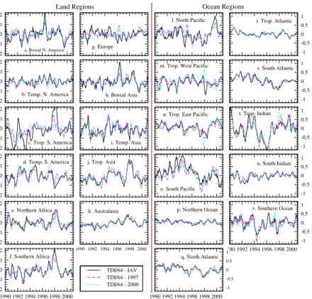
the benefits of using IAV meteorology. Figure4shows the differences in CO₂flux vari-ability due to the use of cyclostationary meteorology corresponding to 1997 (an El Ni ˜no year) and 2000 (a weak positive NAO year) with respect to the IAV meteorology. For most regions the flux variabilities are well captured by using repeating meteorology for the NIES/FRCGC model transport. However, there are also specific regions with

signif-15

icant differences, such the Tropical South America (Fig.4c), Europe (Fig.4g), Tropical East and West Pacific (Figs.4m, n).

The Tropical South America and Tropical East Pacific regions are the areas that experience the largest impact from ENSO related dynamical variations. For exam-ple, during the positive ENSO phase (e.g., 1997/98) the atmospheric regions over the

20

ocean experience greater convective activity associated with warmer sea-surface tem-peratures (SST), which causes less intense easterly winds (Shu and Clarke, 2002). During this period, Tropical South America becomes dryer and less convective. This condition probably weakens the link between Tropical South American flux variability and the CO₂ measurements at the Pacific Ocean sites (see Fig. 1). The opposite

25

condition is in effect during the neutral or negative ENSO periods. This suggests that the TDI/64-2000 inversion produces the least flux variability for Tropical South America because the contribution of transport model simulated signals to concentrations at the

ACPD

Full Screen / Esc

Printer-friendly Version Interactive Discussion measurement sites are greater due to smaller basis-region flux variations. We

there-fore conclude that using repeating meteorology from a non-ENSO year could lead to an under- or over-estimate of the inter-annual variability associated with the Tropical South America or other regions.

The TDI/64-1997 results for Tropical South American flux anomaly are in good

agree-5

ment with the TDI/64-IAV until about December 1997, but quickly deviated from the TDI/64-IAV flux anomalies after this point (Fig. 4c) and agree more closely with the TDI/64 flux anomalies using 1998 meteorology (not shown). The TDI/64-2000 result fails to capture clearly a positive flux anomaly for the 1997/98 El Ni ˜no period from this region. This is because the meteorology for the first half of 1997 does not have positive

10

ENSO signatures. The use of cyclostationary meteorology could be one of the main reasons that no significant positive flux was anomaly deduced by Baker et al. (2005) for Tropical South America. Flux estimates for Tropical Asia, the other region of strong CO₂ emission due to the El Ni ˜no, is not effected by the selection of transport model dynamics in this study (Fig.4j).

15

The Tropical Pacific flux anomalies are also significantly affected by forward model meteorology. In contrast to the Tropical South American region, the Tropical East Pa-cific flux anomaly is more variable when year 2000 meteorology is used. There are measurement stations (Pacific Ocean cruise) in the western part of this region and the eastern side of the Tropical West Pacific region. Thus, we believe this variability mostly

20

corresponds to the changes in CO₂ fluxes in central Pacific region that is captured by the observing stations under this ATM INV modelling framework. The strong negative flux anomaly (∼1.0 Pg-C) in late 1997 by TDI/64-2000 compared to TDI/64-IAV is prob-ably exaggerated because Feely et al. (1999) have estimated a flux anomaly change of about 0.7 Pg-C between 1996 and 1997. Such a situation also forces a compensatory

25

positive flux anomaly in the Tropical West Pacific region (Figs.4m, n).

The other dominant climate oscillation is the NAO, which may play a major role in controlling the European CO₂ flux variability (Patra et al., 2005b). We find that us-ing variable meteorology plays a crucial role in the determination of interannual flux

ACPD

Full Screen / Esc

Printer-friendly Version Interactive Discussion variability in Europe (Fig.4g). For instance, the largest discrepancy in flux anomalies

occurs during the winter of 1996–1997, which was a period of strong negative NAO. The negative NAO phase brings humid air into the Mediterranean and cold air to north-ern Europe (Hurrel et al., 2003). The wetter weather in south-west Europe leads to a weak negative flux anomaly due to enhanced biological uptake (not shown), and the

5

colder weather in the north-west Europe probably decreased the heterotrophic respi-ration that results in a strong negative flux anomaly of CO₂. These results are based on 4-sub regional fluxes of Europe in TDI/64-IAV case. A negative flux anomaly during the 1996–1997 period is seen in the results of TDI/64-IAV, but the opposite behavior in the CO₂flux anomaly is derived using cyclostationary meteorology. In these cases,

10

south-west Europe becomes a stronger source of CO₂ (not shown), which is highly unlikely given the relatively wet climate associated with a negative NAO. Nevertheless, the cause of the differences between TDI/64-IAV and the simulations using repeating meteorology is not straightforward to explain with atmospheric transport due to the complexity of transport in this area as observed at the surrounding measurement sites.

15

3.3 TTM simulations of CO₂ seasonal cycles and growth rates using different flux scenarios

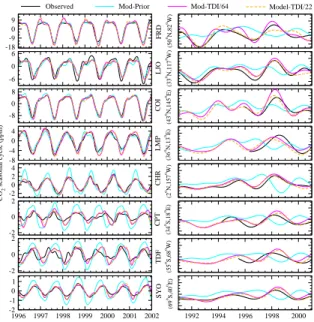
Figure5shows the interannual variability in CO₂seasonal cycles and growth rates as observed (GLOBALVIEW-CO₂, 2005) and simulated by the NIES/FRCGC tracer trans-port model at several stations. Most of these stations data (except COI, SYO) are not

20

used in the TDI model simulations, and are widely distributed around the globe with multiyear measurement records. Thus this set of stations is fairly ideal for our vali-dation test. As expected, the fit to observed seasonal cycles and growth rates for all stations have improved significantly by applying the TDI model flux corrections to the prior flux distributions. Note here that the prior fluxes do not have any interannual

vari-25

ability, and thus the interannual variations in the model simulations are arising entirely from the IAV component in transport model meteorology. For most of the stations, the TDI/64-IAV flux simulations fit the observations better than the simulations using

ACPD

Full Screen / Esc

Printer-friendly Version Interactive Discussion TDI/22-IAV. However, the simulations using TDI/64-IAV fluxes slightly overestimate the

growth rates at the southern extratropical stations after about 1997/98. The growth rates at CPT, TDF, and SYO are systematically greater by a few tenths of a ppm (Fig.5, right columns). This suggests that the TDI model flux during 1997–98 is overestimated by several tenths of a Pg-C globally. For all stations, the observed seasonal cycles are

5

much better matched by the simulations using inverted fluxes in comparison with the prior flux simulations. The seasonal amplitudes produced by prior flux simulations are larger than the observed ones except at the northern high-latitude land stations, FRD and LJO.

We have estimated the goodness-of-fit (defined as: χ2

=(Observations-10

Simulations)2/Number of time intervals) of the simulated growth rates and seasonal cycles to the observations (Table2). The χ2values corresponding to TDI/64-IAV fluxes but with faster vertical diffusion coefficient (TDI/64-FD) are also given. A recent study (Gurney et al., 2004) suggested that the NIES/FRCGC model produced greater than multimodel averaged seasonal amplitude in northern extratropical CO₂. Thus,

TDI/64-15

FD case is conducted to test impact of vertical diffusion on transport model results. It is observed that by increasing the vertical diffusion rate, the fit between both observed seasonal cycles and growth rates have improved for TDI/64-FD simulations compared to that for the TDI/64-IAV. The improvement in fit is the greatest for the FRD station, located in the middle of a continent. All other stations are mostly sampling marine

20

air. The stability of the planetary boundary layer (PBL) at FRD is the greatest during winter (Chen et al., 2005). In general, this is true for all the northern extratropical land regions, which are mainly influenced by the increase in the minimum diffusion rate. In the NIES/FRCGC model, the vertical diffusion rates are frequently greater than 120 m2s−1 for most other regions. Overall, no such differences in the fit of the growth

25

ACPD

Full Screen / Esc

Printer-friendly Version Interactive Discussion

4 Conclusions

We have estimated monthly-mean fluxes of CO₂for the period 1988–2001 using time-dependent ATMOS-INV and forward model simulations driven by different meteorol-ogy. The long-term mean fluxes derived using the maximum possible number of at-mospheric observations are in good agreement with the sea-air CO₂ flux estimates

5

based on an ocean inverse approach that is entirely independent of the atmospheric inversion. The TDI inverse fluxes and flux variabilities are then used for transport model simulations of atmospheric-CO₂. The model and observations are a better match when TDI modeled fluxes are used in TTM simulations compared to those obtained using prior knowledge of CO₂fluxes (fossil fuel emission, CASA biospheric flux, and oceanic

10

exchange). These results suggests an overall validity of TDI model fluxes based on atmospheric-CO₂.

Acknowledgements. Preliminary analyses were first presented in TransCom 3 meetings;

Tsukuba (2004) and Paris (2005) (PPT files available athttp://www.purdue.edu/transcom

fol-lowing appropriate links from the L.H.S. menu bar). Discussions regarding the TransCom upper 15

air experiment have influenced organisation of this article. Support of H. Akimoto for this re-search is appreciated. We used the Earth Simulator, under the support of JAMSTEC, for TTM simulations.

References

Bacastow, R. B.: Dip in the atmospheric CO₂level during the mid-1960’s, J. Geophys. Res.,

20

80, 3109–3114, 1979.

Baker, D., Law, R. M., Gurney, K. R., Denning, A. S., Rayner, P. J., Pak, B. C., Bousquet, P., Bruhwiler, L., Chen, Y.-H., Ciais, P., Fung, I. Y., Heimann, M., John, J., Maki, T., Maksyutov, S., Peylin, P., Prather, M., and Taguchi, S.: Transcom 3 inversion intercomparison: Model mean results for the estimation of seasonal carbon sources and sinks, Global Biogeochem. 25

Cycles, 18, GB1010, doi:10.1029/2004GB00243, 2006.

ACPD

Full Screen / Esc

Printer-friendly Version Interactive Discussion

Bousquet, P., Peylin, P., Ciais, P., Qu ´er ´e, C. L., Friedlingstein, P., and Tans, P.: Regional changes in carbon dioxide fluxes of land and ocean since 1980, Science, 290, 1342–1346, 2000.

Chen, B., Chen, J. M., and Worthy, D. E. J.: Interannual variability in the

atmo-spheric CO₂ rectification over a boreal forest region, J. Geophys. Res., 110, D16301,

5

doi:10.1029/2004JD005546, 2005.

Conway, T. J., Tans, P. P., Waterman, L. S., Thoning, K. W., Kitzis, D. R., Masarie, K. A., and Zhang, N.: Evidence for interannual variability of the carbon cycle from the NOAA/CMDL global air sampling network, J. Geophys. Res., 99, 22 831–22 855, 1994.

GLOBALVIEW-CO2: Cooperative Atmospheric Data Integration Project – Carbon Dioxide.

CD-10

ROM, NOAA CMDL, Boulder, Colorado (anonymous FTP to ftp://ftp.cmdl.noaa.gov, path:

ccg/CO2/GLOBALVIEW), 2002.

Gloor, M., Gruber, N., Hughes, T. M. C., and Sarmiento, J. L.: An inverse modeling method for estimation of net air-sea fluxes from bulk data: Methodology and application to the heat cycle, Global Biogeochem. Cycles, 15, 767, doi:10.1029/2000GB001301, 2001.

15

Gloor, M., Gruber, N., Sarmiento, J. L., Sabine, C. L., Feely, R. A., and R ¨odenbeck,

C. R.: A first estimate of present and preindustrial air-sea CO₂ flux patterns based

on ocean interior carbon measurements and models, Geophys. Res. Lett., 30(1), 1010, doi:10.1029/2002GL015594, 2003.

Gurney, K. R., Law, R. M., Denning, A. S., Rayner, P. J., Pak, B. C., Baker, D., Bousquet, P., 20

Bruhwiler, L., Chen, Y.-H., Ciais, P., Fung, I. Y., Heimann, M., John, J., Maki, T., Maksyutov, S., Peylin, P., Prather, M., and Taguchi, S.: Transcom 3 inversion intercomparison: Model mean results for the estimation of seasonal carbon sources and sinks, Global Biogeochem. Cycles, 18, GB1010, doi:10.1029/2003GB002111, 2004.

Houghton, R. A.: Revised estimates of the annual net flux of carbon to the atmosphere from 25

changes in land use and land manangement 1850–2000, Tellus, 55B, 378–390, 2003. Hurrell, J. W., Kushnir, Y., Visbeck, M., and Ottersen, G.: An Overview of the North Atlantic

Oscillation, The North Atlantic Oscillation: Climate Significance and Environmental Impact, Geophysical Monograph Series 134, edited by: Hurrell, J. W., Kushnir, Y., Ottersen, G., and Visbeck, M., 1–35, 2003.

30

Jones, C. D. and Cox, P. M.: On the significance of atmospheric CO₂growth rate anomalies in

2002–2003, Geophys. Res. Lett., 32, L14816, doi:10.1029/2005GL023027, 2005.

ACPD

Full Screen / Esc

Printer-friendly Version Interactive Discussion

of rise of atmospheric carbon dioxide since 1980, Nature, 375, 666–670, 1995.

Keeling, C. D., Chin, J. F. S., and Whorf, T. P.: Increased activity of northern vegetation inferred

from atmospheric CO₂measurements, Nature, 382, 146–149, 1996.

Levin, I., Kromer, B., Schmidt, M., and Sartorius, H.: A novel approach for independent

bud-geting of fossil fuels CO2 over Europe by14CO₂observations, Geophys. Res. Lett., 30(23),

5

2194, doi:10.1029/2003GL018477, 2003.

Maksyutov, S. and Inoue, G.: Vertical profiles of radon and CO₂ simulated by the global

at-mospheric transport model, CGER supercomputer activity report, CGER/NIES-I039-2000, 7, 39–41, 2000.

Marland, G., Boden, T. A., and Andres, R. J.: Global, Regional, and National Fossil Fuel CO₂

10

Emissions, in: Trends: A Compendium of Data on Global Change C.D.I.A.C., Oak Ridge National Lab., Oak Ridge, 2003.

Masarie, K. A. and Tans, P. P.: Extension and integration of atmospheric carbon dioxide data into a globally consistent measurement record, J. Geophys. Res., 100(D6), 11 593–11 610, 1995.

15

Matsueda, H., Inoue, H. Y., and Ishii, M.: Aircraft observation of carbon dioxide at 8–13 km altitude over the western Pacific from 1993 to 1999, Tellus, 54B, 1–21, 2002.

McKinley, G. A., R ¨odenbeck, C., Gloor, M., Houweling, S., and Heimann, M.: Pacific dominance to global air-sea CO2 flux variablility: A novel atmospheric inversion agress with ocean mod-els, Geophys. Res. Lett., 31, GL22308, doi:10.1029/2004GL021069, 2004.

20

Mikaloff Fletcher, S. E., Gruber, N., Jacobson, A. R., Doney, S. C., Dutkiewicz, S., Gerber, M., Follows, M., Joos, J., Lindsay, K., Menemenlis, D., Mouchet, A., M ¨uller, S. A., and Sarmiento,

J. L.: Inverse estimates of anthropogenic CO2uptake, transport, and storage by the ocean,

Global Biogeochem. Cycles, 20, GB2002, doi:10.1029/2005GB002530, 2006a.

Nakazawa, T., Ishizawa, M., Higuchi, K., and Trivett, N. B. A.: Two curvefitting methods applied 25

to CO₂flask data, Environmetrics, 8, 197–218, 1997.

Patra, P. K., Maksyutov, S., and Nakazawa, T.: Analysis of atmospheric CO₂ growth rates at

Mauna Loa using inverse model derived CO₂fluxes, Tellus, 57B, 357–365, 2005.

Patra, P. K., Maksyutov, S., Ishizawa, M., Nakazawa, T., Takahashi, T., and Ukita, J.:

Interan-nual and decadal changes in the sea-air CO₂flux from atmospheric CO₂inverse modelling,

30

Global Biogeochem. Cycles, 19, GB4013, doi:10.1029/2004GB002257, 2005a.

Patra, P. K., Ishizawa, M., Maksyutov, S., Nakazawa, T., and Inoue, G.: Role of biomass burning and climate anomalies for land-atmosphere carbon fluxes based on inverse modeling of

ACPD

Full Screen / Esc

Printer-friendly Version Interactive Discussion

atmospheric CO₂, Global Biogeochem. Cycles, 19, GB3005, doi:10.1029/2004GB002258,

2005b.

Patra, P. K., Gurney, K. R., Denning, A. S., Maksyutov, S., Nakazawa, T., Baker, D., Bousquet, P., Bruhwiler, L., Chen, Y.-H., Ciais, P., Fan, S.-M., Fung, I. Y., Gloor, M., Heimann, M., Higuchi, K., John, J., Law, R. M., Maki, T., Pak, B. C., Peylin, P., Prather, M., Rayner, P. J., 5

Sarmiento, J. L., Taguchi, S., Takahashi, T., and Yuen, C.-W.: Sensitivity of inverse estimation

of annual mean CO₂ sources and sinks to ocean-only sites versus all-sites observational

networks, Geophys. Res. Lett., 33, L05814, doi:10.1029/2005GL025403, 2006.

Peylin P., Bousquet, P., Le Qu ´er ´e, C., Sitch, S., Friedlingstein, P., McKinley, G., Gruber, N.,

Rayner, P., and Ciais, P.: Multiple constraints on regional CO₂ flux variations over land and

10

oceans, Global Biogeochem. Cycles, 19, GB1011, doi:10.1029/2003GB002214, 2005. Rayner, P. J., Enting, I. G., Francey, R. J., and Langenfelds, R.: Reconstructing the recent

carbon cycle from atmospheric CO2, δ

13

C and O2/N2observations, Tellus, 51B, 213–232,

1999.

R ¨odenbeck, C., Houweling, S., Gloor, M., and Heimann, M.: Time-dependent atmospheric CO₂

15

inversions based on interannually varying tracer transport, Tellus, 55B, 488–497, 2003a.

R ¨odenbeck, C., Houweling, S., Gloor, M., and Heimann, M.: CO₂ flux history 1982–2001

inferred from atmospheric data using a global inversion of atmospheric transport, Atmos. Chem. Phys., 3, 1919–1964, 2003b.

Takahashi, T., Sutherland, S. C., Sweeney, C., Poisson, A., Metzl, N., Tilbrook, B., Bates, N., 20

Wanninkhof, R., Feely, R. A., Sabine, C., Olafsson, J., and Nojiri, Y.: Global sea-air CO₂

flux based on climatological surface ocean pCO₂, and seasonal biological and temperature

effects, Deep-Sea Res. Part II, 49, 1601–1622, 2002.

Tans, P. P., Fung, I. Y., and Takahashi, T.: Observational constraints on the global atmospheric carbon dioxide budget, Science, 247, 1431–1438, 1990.

25

Walker, G. T.: Correlation in seasonal variations of weather, II, Memoirs of the Indian Meteoro-logical Department, 21 (Part 2), 22–45, 1910.

ACPD

Full Screen / Esc

Printer-friendly Version Interactive Discussion Table 1. Comparison of flux estimates and uncertainties for the ocean regions using the

atmospheric-CO₂ observations at 87 stations (averaging period: 1988–2001) and ocean

in-verse models (PKP05: Patra et al., 2005a; SMF06: Mikaloff Fletcher et al., 2006a, b1

). The average fluxes from ATMOS-INV using three additional observational networks with 76, 67 and

19 stations are also given (see Fig.1). All the values are in Pg-C yr−1.

SMF06 PKP05 Net: 75 station Net: 67 station Net: 19 station

Flux region Flux Unc. Flux Unc. Flux Unc. Flux Unc. Flux Unc.

North Pacific −0.42 0.10 −0.30 0.56 −0.26 0.86 −0.26 0.86 −0.88 1.18

Tropical West Pacific 0.08 0.08 −0.08 0.45 −0.17 0.61 −0.17 0.61 −0.18 0.77

Tropical East Pacific 0.30 0.09 0.39 0.54 0.19 0.77 0.19 0.77 0.33 1.05

South Pacific −0.44 0.11 −0.59 0.71 0.66 1.05 0.66 1.05 −0.25 2.16

Northern Ocean −0.17 0.09 −0.40 0.30 −0.29 0.45 −0.29 0.45 −0.44 0.47

North Atlantic −0.32 0.08 −0.32 0.44 −0.25 0.63 −0.25 0.63 −0.34 0.71

Tropical Atlantic 0.14 0.11 0.16 0.49 0.19 0.70 0.19 0.70 0.21 0.71

South Atlantic −0.17 0.05 0.06 0.58 0.01 0.83 0.01 0.83 0.03 0.86

Tropical Indian Ocean 0.10 0.08 −0.15* 0.77 −0.11 1.10 −0.11 1.10 −0.07 1.13

South Indian Ocean −0.48 0.08 −0.46 0.55 −0.42 0.79 −0.42 0.79 −0.57 0.90

Southern Ocean −0.33 0.21 −0.41 0.79 −0.49 1.10 −0.49 1.10 −0.05 1.62

Global Ocean −1.70 0.52 −2.11 0.52 −0.95 0.58 −0.95 0.68 −2.22 0.97

*This value becomes −0.04 Pg-C yr−1 if the unusual flux anomaly period of 1995−1996 is

excluded (ref. Fig.4). During this period, there was a known problem in the observations at

Seychelles station (5◦N, 55◦E), and the air sampling protocol has since been rectified (T.

Con-way, personal communication, Jena, 2003).

ACPD

Full Screen / Esc

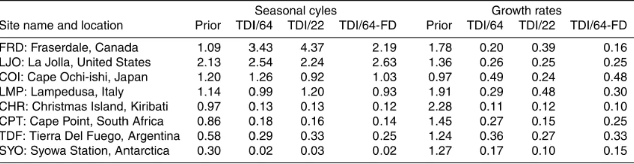
Printer-friendly Version Interactive Discussion Table 2. Goodness-of-fit (χ2) between the observed CO₂ values and NIES/FRCGC model

simulated concentrations using, 1. prior flux distributions based on fossil fuel emission, CASA neutral biosphere fluxes, and Takahashi Ocean fluxes (Prior), 2. corrected fluxes using the 64-region TDI model (TDI/64), 3. corrected fluxes using the 22-region TDI model (TDI/22), and 4. TDI/64, but with NIES/FRCGC model diffusion in upper troposphere (TDI/64-FD). The period for this calculation is from 1 January 1996 to 31 December 2000. These dates were selected to avoid data gaps exceeding one year.

Seasonal cyles Growth rates

Site name and location Prior TDI/64 TDI/22 TDI/64-FD Prior TDI/64 TDI/22 TDI/64-FD

FRD: Fraserdale, Canada 1.09 3.43 4.37 2.19 1.78 0.20 0.39 0.16

LJO: La Jolla, United States 2.13 2.54 2.24 2.63 1.36 0.26 0.25 0.25

COI: Cape Ochi-ishi, Japan 1.20 1.26 0.92 1.03 0.97 0.49 0.24 0.48

LMP: Lampedusa, Italy 1.14 0.99 1.20 0.93 1.91 0.29 0.48 0.30

CHR: Christmas Island, Kiribati 0.97 0.13 0.13 0.12 2.28 0.11 0.12 0.10

CPT: Cape Point, South Africa 0.86 0.18 0.16 0.14 1.45 0.27 0.15 0.25

TDF: Tierra Del Fuego, Argentina 0.58 0.29 0.33 0.25 1.24 0.36 0.27 0.33

ACPD

Full Screen / Esc

Printer-friendly Version Interactive Discussion

EGU

8 P. K. Patra et al.: CO2Fluxes, their variability and modelling of atmospheric CO2

180W 120W 60W 0 60E 120E 180E

Longitude 90S 60S 30S 0 30N 60N 90N Latitude 19 stations 67 stations 76 stations 87 stations Bor. N. America Temp. N. America Temp. S. Northern Africa Southern Temperate Asia Boreal Asia Europe Australasia Trop. Asia N. Pacific East Pacific West S. Pacific Southern Ocean S. Ind. Ocean Trop. Ind. Northern Ocean N. Atlantic Trop. Atlantic S. Atlantic America Trop. S. America Africa Pacific Ocean

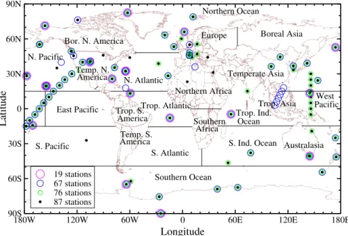
Fig. 1.The atmospheric-CO2measurement networks used in this study are shown. These networks are similar to those used in Bousquet et

al. (2000): 67 stations, TransCom (Gurney et al., 2004): 76 stations, R¨odenbeck et al. (2003b): 19 stations, and Patra et (2005a): 87 stations. The 22 TDI model regions are also shown; the 64-region TDI model has 4 divisions for the land regions (except for Tropical Asia) and the ocean regions are divided into two along the longitude (see Patra et al., 2005a,b for further details).

Atmos. Chem. Phys., 0000, 0001–12, 2006 www.atmos-chem-phys.org/acp/0000/0001/

Fig. 1. The atmospheric-CO₂ measurement networks used in this study are shown. These networks are similar to those used in Bousquet et al. (2000): 67 stations, TransCom (Gurney et al., 2004): 76 stations, R ¨odenbeck et al. (2003b): 19 stations, and Patra et (2005a): 87 stations. The 22 TDI model regions are also shown; the 64-region TDI model has 4 divisions for the land regions (except for Tropical Asia) and the ocean regions are divided into two along the longitude (see Patra et al., 2005a, b, for further details).

ACPD

Full Screen / Esc

Printer-friendly Version Interactive Discussion 352 356 360 364 368 372 CO 2 [ppm]

Obs. conc.: GlobalView Conc. fitted: Daily Trend fitted: daily

1991 1992 1993 1994 1995 1996 1997 1998 1999 2000 2001 Calendar Year -4 -2 0 2 4 CO 2 [ppm]

Seasonal Cycle: Fit - Trend

Growth rate: trend (t=n+182) - trend (t=n-182) a

b

Fig. 2. An example of the extraction of seasonal cycles and growth rates (b) from

ACPD

Full Screen / Esc

Printer-friendly Version Interactive Discussion Fig. 3. Comparison of CO₂flux estimates using an ocean inversion and atmospheric inversions

using different modeling frameworks. The regional fluxes of higher resolution inverse models

are aggregated to TransCom-3 regions (subcontinental scale). R ¨odenbeck et al. (2003) fluxes are the average of the inversion cases used in this study (refer to their Fig. 8) and correspond to the 1990s. Gurney et al. (2004) and Baker et al. (2006) fluxes correspond to the periods 1992–1996 and 1991–2000, respectively.

ACPD

Full Screen / Esc

Printer-friendly Version Interactive Discussion

P. K. Patra et al.: CO2Fluxes, their variability and modelling of atmospheric CO2 11

-2 -1 0 1 2 -1 -0.5 0 0.5 1 -2 -1 0 1 2 -1 -0.5 0 0.5 1 -2 -1 0 1 2 -1 -0.5 0 0.5 1 -2 -1 0 1 2 -1 -0.5 0 0.5 1 -2 -1 0 1 2 1990 1992 1994 1996 1998 2000 ’90 1992 1994 1996 1998 2000 -1 -0.5 0 0.5 1 1990 1992 1994 1996 1998 2000 -2 -1 0 1 2 TDI/64 - IAV TDI/64 - 1997 TDI/64 - 2000 1990 1992 1994 1996 1998 2000 -1 -0.5 0 0.5 1

Land Regions Ocean Regions

a. Boreal N. America b. Temp. N. America c. Trop. S. America d. Temp. S. America e. Northern Africa f. Southern Africa g. Europe h. Boreal Asia i. Temp. Asia j. Trop. Asia k. Australasia l. North Pacific

m. Trop. West Pacific

n. Trop. East Pacific

o. South Pacific p. Northern Ocean q. North Atlantic r. Trop. Atlantic s. South Atlantic t. Trop. Indian u. South Indian v. Southern Ocean

Fig. 4.A comparison of CO2flux anomalies for 22 regions of the globe is shown (11 land: two left columns, and 11 ocean: two right columns); fluxes are derived using the 64-region TDI model with varying TTM meteorology. A long-term mean seasonal cycle for each region is subtracted from the TDI model derived monthly fluxes to calculate the anomalies. Five-month running averages are taken to reduce the high frequency variability in fluxes and all values on the y-axis (flux anomaly) are in Pg-C yr−1_{. Two common y-axis scales (on the left} and on right) are used for the land and ocean fluxes, respectively.

www.atmos-chem-phys.org/acp/0000/0001/ Atmos. Chem. Phys., 0000, 0001–12, 2006

Fig. 4. A comparison of CO₂ flux anomalies for 22 regions of the globe is shown (11 land: two left columns, and 11 ocean: two right columns); fluxes are derived using the 64-region TDI model with varying TTM meteorology. A long-term mean seasonal cycle for each region is subtracted from the TDI model derived monthly fluxes to calculate the anomalies. Five-month running averages are taken to reduce the high frequency variability in fluxes and all values on

the y-axis (flux anomaly) are in Pg-C yr−1. Two common y-axis scales (on the left and on right)

ACPD

Full Screen / Esc

Printer-friendly Version Interactive Discussion -18 -9 0 9 -6 0 6 -8 0 8 -8 -4 0 4 -2 0 2 4 CO 2 seasonal cycle (ppm) -2 0 2 -2 0 2 1996 1997 1998 1999 2000 2001 2002 -2 -1 0 1 1992 1994 1996 1998 2000 FRD LJO COI LMP CHR CPT TDF SYO

Observed Mod-Prior Mod-TDI/64 Model-TDI/22

(69 oS,40 oE) (55 oS,68 oW) (34 oS,18 oE) (2 oN,157 oW) (36 oN,13 oE) (43 oN,145 oE) (33 oN,117 oW) (50 oN,82 oW)

Fig. 5. Timeseries of observed seasonal cycles (left column) and growth rates (right column)

at 8 stations worldwide are compared with NIES/FRCGC model simulations using three flux scenarios. The observed curves are shown for the periods with data gaps less than an year. Note that the seasonal cycles and growth rates are shown for different period for better clarity. In addition, the y-axis ranges are different for each panel on left column. The abbreviated

sta-tion names and locasta-tions (latitude, longitude) are given between the two columns (see Table2

for full names). The CO₂data are obtained from following organisations for GlobalView

analy-sis; FRD: Meteorological Service of Canada (MSC), LJO: Scripps Institution of Oceanography (SIO), United States, COI: National Institute for Environmental Studies (NIES), Japan, LMP: Na-tional Agency for New Technology, Energy, and Environment (ENEA), Italy, CHR: NOAA/Global Monitoring Division (GMD), United States, CPT: South African Weather Service (SAWS), TDF: NOAA/Global Monitoring Division (GMD), and SYO: National Institute of Polar Research in

cooperation with Tohoku University (NIPR/TU), Japan (see the GLOBALVIEW-CO₂

documen-tation for further details).