HAL Id: hal-01584259
https://hal.archives-ouvertes.fr/hal-01584259
Submitted on 27 Oct 2020
HAL is a multi-disciplinary open access
archive for the deposit and dissemination of
sci-entific research documents, whether they are
pub-lished or not. The documents may come from
teaching and research institutions in France or
abroad, or from public or private research centers.
L’archive ouverte pluridisciplinaire HAL, est
destinée au dépôt et à la diffusion de documents
scientifiques de niveau recherche, publiés ou non,
émanant des établissements d’enseignement et de
recherche français ou étrangers, des laboratoires
publics ou privés.
Chemistry and Physics, European Geosciences Union, 2017, 17 (13), pp.8371 - 8394.
�10.5194/acp-17-8371-2017�. �hal-01584259�
https://doi.org/10.5194/acp-17-8371-2017 © Author(s) 2017. This work is distributed under the Creative Commons Attribution 3.0 License.
Detectability of Arctic methane sources at six sites performing
continuous atmospheric measurements
Thibaud Thonat1, Marielle Saunois1, Philippe Bousquet1, Isabelle Pison1, Zeli Tan2, Qianlai Zhuang3,
Patrick M. Crill4, Brett F. Thornton4, David Bastviken5, Ed J. Dlugokencky6, Nikita Zimov7, Tuomas Laurila8, Juha Hatakka9, Ove Hermansen9, and Doug E. J. Worthy10
1Laboratoire des Sciences du Climat et de l’Environnement, LSCE/IPSL, CEA-CNRS-UVSQ,
Université Paris-Saclay, 91191 Gif-sur-Yvette, France
2Pacific Northwest National Laboratory, Richland, Washington, USA
3Department of Earth, Atmospheric, and Planetary Sciences, Purdue University, West Lafayette, Indiana, USA 4Department of Geological Sciences and Bolin Centre for Climate Research, Svante Arrhenius väg 8,
106 91, Stockholm, Sweden
5Department of Thematic Studies – Environmental Change, Linköping University, 581 83 Linköping, Sweden 6NOAA Earth System Research Laboratory, Global Monitoring Division, Boulder, Colorado, USA
7Northeast Science Station, Cherskiy, Russia
8Climate and Global Change Research, Finnish Meteorological Institute, Helsinki, Finland 9NILU – Norwegian Institute for Air Research, Kjeller, Norway
10Environment Canada, Toronto, Ontario, Canada
Correspondence to:Thibaud Thonat ([email protected]) Received: 24 February 2017 – Discussion started: 9 March 2017
Revised: 6 June 2017 – Accepted: 9 June 2017 – Published: 11 July 2017
Abstract. Understanding the recent evolution of methane emissions in the Arctic is necessary to interpret the global methane cycle. Emissions are affected by significant uncer-tainties and are sensitive to climate change, leading to poten-tial feedbacks. A polar version of the CHIMERE chemistry-transport model is used to simulate the evolution of tropo-spheric methane in the Arctic during 2012, including all known regional anthropogenic and natural sources, in par-ticular freshwater emissions which are often overlooked in methane modelling. CHIMERE simulations are compared to atmospheric continuous observations at six measurement sites in the Arctic region. In winter, the Arctic is domi-nated by anthropogenic emissions; emissions from continen-tal seepages and oceans, including from the East Siberian Arctic Shelf, can contribute significantly in more limited areas. In summer, emissions from wetland and freshwater sources dominate across the whole region. The model is able to reproduce the seasonality and synoptic variations of methane measured at the different sites. We find that all methane sources significantly affect the measurements at all
stations at least at the synoptic scale, except for biomass burning. In particular, freshwater systems play a decisive part in summer, representing on average between 11 and 26 % of the simulated Arctic methane signal at the sites. This in-dicates the relevance of continuous observations to gain a mechanistic understanding of Arctic methane sources. Sen-sitivity tests reveal that the choice of the land-surface model used to prescribe wetland emissions can be critical in cor-rectly representing methane mixing ratios. The closest agree-ment with the observations is reached when using the two wetland models which have emissions peaking in August– September, while all others reach their maximum in June– July. Such phasing provides an interesting constraint on wet-land models which still have large uncertainties at present. Also testing different freshwater emission inventories leads to large differences in modelled methane. Attempts to in-clude methane sinks (OH oxidation and soil uptake) reduced the model bias relative to observed atmospheric methane. The study illustrates how multiple sources, having different spatiotemporal dynamics and magnitudes, jointly influence
widely debated (e.g. Nisbet et al., 2014). A number of differ-ent processes have been examined including changes in an-thropogenic sources (Schaefer et al., 2016; Hausmann et al., 2016; Schwietzke et al., 2016), in natural wetlands (Bous-quet et al., 2011; Nisbet et al., 2016, McNorton et al., 2016), or in methane lifetime (Dalsøren et al., 2016; Rigby et al., 2017; Turner et al., 2017).
Recent changes in methane concentrations are not uni-form and vary with latitude. The rise in methane in 2007 was, for example, particularly important in the Arctic re-gion due to anomalously high temperatures leading to high wetland emissions (Dlugokencky et al., 2011; Bousquet et al., 2011). The Arctic (> 60◦N) is of particular interest given the size of its carbon reservoirs and the amplitude of recent and projected climate changes. It sequesters about 50 % of the global organic soil carbon (Tarnocai et al., 2009). De-composition of its most superficial fraction can lead to im-portant feedbacks to climate warming. The Arctic is already affected by an amplification of climate warming; warming there is about twice that of the rest of the world (Christensen et al., 2013). Between 1950 and 2012, combined land and sea-surface mean temperature had increased by about 1.6◦C in the region (AMAP, 2015), and climate projections predict temperature changes of a few degrees over the next decades (Collins et al., 2013). The Arctic now represents about 4 % of the global methane budget (23 vs. 568 TgCH4yr−1for 2012,
according to Saunois et al., 2016). This budget is lower than bottom-up estimates (range 37–89 TgCH4yr−1, according to
the review by Thornton et al., 2016b), which are affected by large uncertainties. Although there is no sign of dramatic per-mafrost carbon emissions yet (Walter Anthony et al., 2016), thawing permafrost could double the 21st century’s Arctic methane budget and impact climate for centuries (Schuur et al., 2015).
This context points to the need to closely monitor Arc-tic sources. The largest individual natural source from high latitudes is wetlands. An ensemble of process-based land-surface models indicate that, between 2000 and 2012, wetland emissions have increased in boreal regions by 1.3 TgCH4, possibly due to increases in wetland area and
lakes are located north of 45◦N (Walter et al., 2007) and their emissions are expected to increase under a warming climate (Wik et al., 2016). Estimates for the high latitudes, extrap-olated from measurements from different samples of lakes can vary from 13.4 TgCH4yr−1 (above 54◦N, Bastviken et
al., 2011) to 24.2 TgCH4yr−1 (above 45◦N, Walter et al.,
2007). Based on a synthesis of 733 measurements made in Scandinavia, Siberia, Canada, and Alaska, Wik et al. (2016) have assessed emissions north of 50◦N at 16.5 TgCH4yr−1.
They have also highlighted the emissions’ dependence on the water body type. Using a process-based lake biogeochem-ical model, Tan and Zhuang (2015a) have come to an es-timate of 11.9 TgCH4 yr−1 north of 60◦N, in the range of
previous studies. This important source is generally repre-sented poorly or not at all in large-scale atmospheric studies (Kirschke et al., 2013).
Additional continental sources include anthropogenic emissions, mostly from Russian fossil fuel industries, and to a lesser extent, biomass burning, mostly originating from boreal forest fires. The Arctic is also under the influence of transported emissions from midlatitude methane sources, mostly of human origin (e.g. Paris et al., 2010; Law et al., 2014).
Marine emissions from the Arctic Ocean are smaller than terrestrial emissions, but they too are climate sensitive and affected by large uncertainties. Sources within the ocean in-clude emissions from geological seeps, from sediment biol-ogy, from underlying thawing permafrost or hydrates, and from production in surface waters (Kort et al., 2012). The East Siberian Arctic Shelf (ESAS, in the Laptev and East Siberian Seas), which comprises more than a quarter of the Arctic shelf (Jakobsson et al., 2002) and most of subsea per-mafrost (Shakhova et al., 2010), is a large reservoir of car-bon and most likely the biggest emission area (McGuire et al., 2009). Investigations led by Shakhova et al. (2010, 2014) estimated total ESAS emissions from diffusion, ebul-lition, and storm-induced degassing, at 8–17 TgCH4yr−1.
A subsequent measurement campaign led by Thornton et al. (2016a), though not made during a stormy period, failed to observe the high rates of continuous emissions reported by
Shakhova et al. (2014), and instead estimated an average flux of 2.9 TgCH4yr−1. Berchet et al. (2016) also found that such
values were not supported by atmospheric observations, and instead suggested the range of 0.0–4.5 TgCH4yr−1.
The main sink of methane is its reaction with the hydroxyl radical (OH) in the troposphere, which explains about 90 % of its loss. Other tropospheric losses include reaction with atomic chlorine (Cl) in the marine boundary layer (Allan et al., 2007) and oxidation in soils (Zhuang et al., 2013). These sinks vary seasonally, especially in the Arctic atmosphere, and their intensity is at maximum in summer, when Arc-tic emissions are the highest. A good representation of the methane budget thus requires a proper knowledge of these sinks.
As mentioned before, a better understanding of methane sources and sinks and of their variations is critical in the con-text of climate change. Methane emissions can be estimated either by bottom-up studies, relying on extrapolation of flux measurements, on inventories and process-based models, or by top-down inversions which optimally combine atmo-spheric observations, transport modelling, and prior knowl-edge of emissions and sinks. The main input for top-down inversions is measurements of atmospheric methane mixing ratios, either at the surface or from space. Such observa-tions are critical and should be made over long time periods to assess trends and variability. Surface methane monitoring started in the Arctic in the mid-1980s. Although more than 15 sites currently exist, six of them being in continuous op-eration (in addition to tower sites such as the JR-STATION tower network over Siberia; Sasakawa et al., 2010), the ob-servational network remains limited considering the Arctic area and the variety of existing sources (AMAP, 2015).
Retrievals of methane concentrations have been made from space since the mid-2000s, from global and continuous observations. However, at high latitudes, passive spaceborne sounders are limited by the availability of clear-sky spots and by sunlight (for NIR/SWIR instruments), and have been af-fected by persistent biases (e.g. Alexe et al., 2015; Locatelli et al., 2015). This is why only surface measurements, which provide precise and accurate data, are used in this study.
One interesting feature of Arctic methane emissions is that they are generally more distinct spatially and temporally (no or low wetland emissions in winter; anthropogenic emissions all year round) compared to tropical emissions (e.g. in north-ern India). Also, fast horizontal winds more efficiently relate emissions to atmospheric measurements (e.g. Berchet et al., 2016).
Methane modelling studies that rely on Arctic measure-ments have been used, for example, to assess the sensitiv-ity of Arctic methane concentrations to uncertainties in its sources, in particular concerning the seasonality of wetland emissions and the intensity of ESAS emissions (Warwick et al., 2016; Berchet et al., 2016). Top-down inversions have also led to methane surface flux estimates and discussions of their variations. For instance, Thompson et al. (2017) have
found significant positive trends in emissions in northern North America and northern Eurasia over 2005–2013, con-tradicting previous global inversion studies based on a more limited observational network north of 50◦N (Bruhwiler et al., 2014; Bergamaschi et al., 2013).
Combining atmospheric methane modelling using the CHIMERE chemistry-transport model (Menut et al., 2013) and surface observations from six continuous measurement sites, this paper aims to evaluate the information contained in methane observations concerning the type, the intensity, and the seasonality of Arctic sources. The study focuses on 2012, as this is the last year for which wetland emissions are available for a set of models in a controlled framework. Section 2 describes the data and modelling tools used in this study. Section 3 analyses the simulated methane mole frac-tions and investigates their agreement with the observafrac-tions. It also discusses the sensitivity of the model to wetland and freshwater sources, as well as to methane sinks. Section 4 concludes this study.
2 Data and model framework
2.1 Methane observations
Continuous methane measurements for the year 2012, from the six Arctic surface sites, have been gathered. The site characteristics are given in Table 1, and Fig. 1 represents their position in the studied domain. Two sites are consid-ered to be remote background sites: Alert, located in north-ern Canada, where measurements are carried out by Environ-ment Canada (EC), and Zeppelin (Ny-Alesund), located in Svalbard archipelago on a mountaintop, and operated by the Norwegian Institute for Air Research (NILU). NOAA Earth System Research Laboratory (NOAA-ESRL) is responsible for the measurements at Barrow observatory, which is lo-cated in northern Alaska, 8 km north-east of the city of Bar-row, and at Cherskii. Cherskii and Tiksi are located close to the shores of the East Siberian Sea and the Laptev Sea, re-spectively. Pallas is located in northern Finland, with domi-nant influence from Europe. Measurements at these last two sites are carried out by the Finnish Meteorological Insti-tute (FMI). No data were available in Barrow in 2012 after May due to a lapse in funding (Sweeney et al., 2016). Gaps in Cherskii (October–January), Pallas (August–mid-October), and Zeppelin (January–April) data are due to instrument is-sues.
Data from Alert, Barrow, and Pallas were downloaded from the World Data Centre for Greenhouse Gases (WD-CGG, http://ds.data.jma.go.jp/gmd/wdcgg/). Tiksi data were obtained through the NOAA-ESRL IASOA (International Arctic Systems for Observing the Atmosphere) platform (https://esrl.noaa.gov/psd/iasoa/). Zeppelin data were ob-tained via the InGOS (Integrated non-CO2Greenhouse Gas
Observing System) project. Cherskii data were provided by NOAA. All valid data from the sites are used in this study,
Figure 1. Delimitation of the studied Polar domain and location of the six continuous measurement sites used in this study. ALT: Alert. BRW: Barrow. CHS: Cherskii. PAL: Pallas. TIK: Tiksi. ZEP: Zeppelin.
with no filter applied. All data are reported in units of mole fraction, nmol mol−1(abbreviated ppb) on the WMO X2004 CH4mole fraction scale. Observations are available at hourly
resolution at least, but in this study we make use of daily means to focus on synoptic variations, which are more ap-propriate for regional modelling.
2.2 Model description
The CHIMERE Eulerian chemistry-transport model (Vautard et al., 2001; Menut et al., 2013) has been used for simulations of tropospheric methane. It solves the advection–diffusion equation on a regular grid, forced using pre-computed me-teorology. Our domain goes from 39◦N to the Pole but it covers all longitudes only above 64◦N, as it is not regular in
grid cells near the Pole (Berchet et al., 2016). Twenty-nine vertical levels characterize the troposphere, from the surface to 300 hPa (∼ 9000 m), with an emphasis on the lowest lay-ers.
The model is forced by meteorological fields from European Centre for Medium Range Weather Fore-casts (ECMWF) foreFore-casts and reanalyses (http://www. ecmwf.int). These include wind, temperature, and water vapour profiles characterized by 3 h time resolution, a spa-tial resolution of ∼ 0.5◦, and 70 vertical levels in the tropo-sphere. Initial and boundary concentrations come from opti-mized global simulations of the LMDZ general circulation model for 2012 (Locatelli et al., 2015). These fields have a 3 h time resolution and 3.75◦×1.875◦ spatial resolution. They are interpolated in time and space with the grid of the CHIMERE domain.
The model is run with seven distinct tracers: six cor-respond to the different Arctic emission sources (anthro-pogenic, biomass burning, geology & oceans, ESAS, wet-lands, and freshwater systems) and one corresponds to the boundary conditions. This framework allows us to analyse the contribution of each source in the simulated total methane mixing ratio, defined as the sum of each tracer. No chemistry is included in the standard simulations, but a sensitivity test is carried out (see Sect. 3.4).
2.3 Emission scenario
Surface emissions used here stem from a set of various inven-tories, models, and data-driven studies, from which are built a reference scenario, complemented by several sensitivity sce-narios. The different emission sources used are described in Table 2, along with the amount of methane emitted in the studied domain.
All types of anthropogenic emissions are provided by the EDGAR (Emission Database for Global Atmospheric Re-search) v4.2 Fast Track 2010 (FT 2010) data (Olivier and Janssens-Maenhout, 2012), which have a 0.1◦×0.1◦ reso-lution. EDGAR emissions are derived from activity statis-tics and emission factors. Given that the EDGARv4.2FT2010
Table 2. Methane emissions in the studied polar domain, for the reference simulation, and for other scenarios. Total emissions for the reference scenario amount to 68.5 TgCH4.
Emissions Emissions
Type of source Reference scenario (TgCH4) Variant scenarios (TgCH4) Anthropogenic Based on Edgar 2010. 20.5 – –
Olivier and Janssens-Maenhout (2012)
Biomass GFED4.1. 3.1 – –
burning van der Werf et al. (2010)
Geology and Based on Etiope (2015) 4.0 – – oceans
ESAS Based on Berchet et al. (2016) 2.0 – – 10 models from
Poulter et al. (2017) 10.1–58.3
CLM4.5a 31.0
CTEMb 25.2
DLEMc 21.8
Wetlands ORCHIDEE land-surface model. 29.5 JULESd 38.3 (Ringeval et al., 2010, 2011) LPJ-MPIe 58.3
LPJ-wslf 10.1
LPX-Berng 19.4
SDGVMh 26.2
TRIPLEX-GHGi 15.4
VISITj 30.0
Our inventory, based on the 9.3 Based on bLake4Me, Tan et al. (2015) 13.6 Freshwater systems GLWD lakes location map,
Lehner and Döll (2004)
aRiley et al. (2011); Xu et al. (2016).bMelton and Arora (2016).cTian et al. (2010, 2015).dHayman et al. (2014).eKleinen et al. (2012).fHodson et al. (2011). gSpahni et al. (2011).hWoodward and Lomas (2004); Cao et al. (1996).iZhu et al. (2014, 2015).jIto and Inatomi (2012).
emissions are not available for years after 2010, the 2010 values are used for 2012 for every sector but the ones for which FAO (Food and Agriculture Organization, http://www. fao.org/faostat/en/#data/) and BP (http://www.bp.com/) data are available (oil and gas production, fugitive from solid, en-teric fermentation, and manure management). In this latter case, the ratio of 2012 to 2010 is used at the country level to update the EDGAR 2010 emissions. For our domain, prior anthropogenic emissions represent 20.5 TgCH4yr−1, mostly
from the fossil fuel industry. EDGAR anthropogenic emis-sion data are constant all year. Although higher emisemis-sions are expected in winter, particularly due to household heating, im-portant emissions also occur in summer, e.g. from seepages from maintenance and welling work (Berchet et al., 2015). In the absence of more precise information, anthropogenic emissions are kept constant all year.
Biomass burning emissions come from the Global Fire Emissions Database version 4 (GFED4.1) (van der Werf et al., 2010; Giglio et al., 2013) monthly means product. Burned areas estimated from the MODIS spaceborne instrument are combined with the biomass density and the combustion effi-ciency derived from the CASA biogeochemical model, and
with an empirically assessed emission factor. The emissions are provided on a 0.25◦×0.25◦grid. Biomass burning emis-sions are 3.1 TgCH4yr−1in our domain.
Wetland emissions in the reference scenario come from the ORCHIDEE-WET model (Ringeval et al., 2010, 2011), which is derived from the ORCHIDEE global vegetation model (Krinner et al., 2005). The wetland methane flux den-sity is computed for each 0.5◦×0.5◦grid cell based on the
Walter et al. (2001) model. Three pathways of transport (dif-fusion, ebullition, and plant-mediated transport) and oxida-tion are included. Annual emissions from wetlands in our
domain are 29.5 TgCH4yr−1 with the ORCHIDEE model.
The version of ORCHIDEE used in this study comes from Poulter et al. (2017) (see also Saunois et al., 2016), like the 10 other land-surface models used for sensitivity studies (see Sect. 3.2). Following Melton et al. (2013), net methane emissions have been computed under a common protocol; the models use the same wetland extent and climate forc-ings. Wetland area dynamics are based on global wetland data sets produced with the GLWD (Global Lakes and Wet-lands Database), combined with SWAMPS (Surface WAter Microwave Product Series) inundated soil maps. The
emis-Figure 2. (a) Freshwater methane emissions used in the reference simulation. (b) Difference between the inventory based on the bLake4Me lake emission model (Tan and Zhuang, 2015a) and the one used in the reference simulation. For both maps, blank areas in the domain correspond to zero emission.
sions from these 10 other models range from 10.1 up to 58.3 TgCH4yr−1.
Emissions from geological sources, including continental macro- and micro-seepages, and marine seepages, are de-rived from the GLOCOS database (Etiope, 2015). They rep-resent 4.0 TgCH4yr−1in our domain.
ESAS emissions are prescribed following Berchet et al. (2016), and scaled to 2 TgCH4yr−1. Their temporal
vari-ability is underestimated as uniform and constant emis-sions were applied by emission type (hotspots and back-ground) and period (winter/summer), based on Shakhova et al. (2010). In particular, we assume that substantial emissions take place during the ice-covered period through polynyas. Although a part of the emissions in ESAS can be considered geological, all potential sources emitting in ESAS are con-sidered here to be one distinct source.
Since they have generally been represented poorly or not at all in former atmospheric studies, freshwater emissions were built for the purpose of this work. The inventory is based on the GLWD level 3 product (Lehner and Döll, 2004), which provides a map of lake and wetland types at a 30 s (∼ 0.0083◦, or 421 × 922 m at 60◦N) resolution. A total value of 15 TgCH4yr−1was prescribed for freshwater
emis-sions at latitudes above 50◦N, according to several recent studies (e.g. Walter et al. (2007): 24.5 TgCH4yr−1 above
45◦N; Bastviken et al. (2011): 13 TgCH4yr−1above 54◦N;
Wik et al. (2016): 16.5 TgCH4yr−1 above 50◦N; Saunois
et al. (2016): 18 TgCH4yr−1above 50◦N). This value was
uniformly distributed over lake and reservoir grid cells, as-suming that a lake or a reservoir occupies the entire grid cell. This method is simplistic, as the dependence of emissions on lake areas, depths, and types are not taken into account. The seasonality of the emissions is underestimated given that no emission takes place when the lake is frozen, and that the
emission is constant after ice-out. Therefore, our inventory does not allow episodic fluxes such as spring methane bursts (Jammet et al., 2015), and emissions during ice-cover period (Walter et al., 2007). Freeze-up and ice-out dates were es-timated using surface temperature data from the ECMWF ERA-Interim Reanalyses. For each lake or reservoir, freeze-up was assumed to happen after two continuous weeks be-low 0◦C; ice-out, after three continuous weeks above 0◦C. Again, this is a simplification, given that there is no sim-ple relation between air temperature and freeze-up or ice-out (e.g. Livingstone, 1999).
As a result, we built an inventory for freshwater emissions (Fig. 2a), (i) with a total budget of 9.3 TgCH4yr−1in our
do-main, consistent with the range provided by recent literature, (ii) with a regional seasonality which is similar to the one of wetland emissions, and (iii) without overlap with wetland areas, as both use the same GLWD database. The impact of this self-made inventory is also compared with the recently published work from Tan et al. (2015) for Arctic lakes (see Sect. 3.3).
The more recent GLOWABO (Global Water Bodies) database (Verpoorter et al., 2014) has a higher resolution
than the GLWD (0.002 vs. 0.1 km2), and finds a higher
combined global surface area of lakes and reservoirs (5 vs. 2.7 × 10⁶km2)as it takes into account smaller lakes. By us-ing the GLWD product to identify both lake and wetland ar-eas, our freshwater inventory may underestimate the emitting surface area, while the wetland inventories may still include open water fluxes. Double-counting is avoided in terms of area, but not necessarily in terms of emission (Thornton et al., 2016b).
3 Results
3.1 Reference simulation
3.1.1 Source contributions within the domain
A simulation of seven methane tracers is run with CHIMERE for 2012. On top of methane from initial and boundary con-ditions, these include methane from anthropogenic sources, biomass burning, East Siberian Arctic Shelf (ESAS), geol-ogy and oceans (counting as only one source and excluding ESAS), wetlands, and freshwater systems.
The boundary conditions are the dominant signal; they re-sult from emissions coming from sources located outside of the domain, and from emissions coming from Arctic sources, which have once left the domain and then re-entered in it. The boundary condition tracer does not hold information on where the transported methane initially comes from. So, to focus on Arctic sources, the source contributions are defined here relatively to the sum of the six tracers which correspond to sources located in the domain, i.e. excluding methane re-sulting from the boundary conditions. The source contribu-tion is only calculated when methane directly from Arctic sources is greater than 1 ppb. One should keep in mind that this signal represents a small fraction of total atmospheric methane.
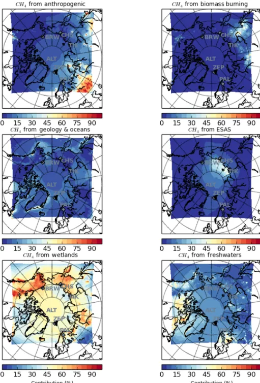
The weight of each source varies both spatially and sea-sonally. Figures 3 and 4 represent the mean source contribu-tions to methane concentracontribu-tions near the surface, in winter (November to May) and in summer (from June to October), respectively.
In winter, anthropogenic methane is dominant (over win-ter, the daily average over the domain is in the range 18– 59 %, with a mean of 42 %). More than 80 % of anthro-pogenic emissions come from oil, gas, and coal industries. In particular, it affects western Russia (mostly due to gas production), the Khanty–Mansia region (mostly due to oil production), and south-eastern Russia (mostly due to coal mining). Oil production is also the main contributor to at-mospheric methane in continental Canada.
Geological and oceanic emissions represent an important part of atmospheric methane in the domain, particularly in winter (11–36 %, mean: 27 %). Emissions from ESAS are expected to be larger in summer, when most of the area is ice-free, than in winter. However, its relative contribution is higher in winter (8–23 %, mean: 15 %), when other sources, particularly from wetlands, are lower. Alaska and northern Siberia are particularly affected by geological and oceanic emissions in winter, including from ESAS.
In summer, wetland emissions are the dominant contrib-utor (33–56 %, mean: 50 %) (although anthropogenic emis-sions remain important in western Russia), while they are quite negligible in winter. Freshwater systems too are an im-portant contributor in summer (9–29 %, mean: 19 %), but of lower intensity than wetlands, except in eastern Canada and
Scandinavia, where methane from lakes can exceed methane from wetlands.
Biomass burning takes place in summer (0–7 %, mean: 4 %), when fuel characteristics and meteorological condi-tions foster combustion. Although the 2012 fire emissions are particularly high (e.g. almost twice as high as the 2013 emissions) and large-scale fires occur in boreal Russian and Canadian forests, their impact on methane remains limited to some regions in continental Russia.
3.1.2 Arctic source contributions at atmospheric
monitoring sites
The contribution of the different sources is more quantita-tively discussed in the following, focusing on the six contin-uous measurement sites shown in Figs. 3 and 4.
The evolution of the daily averaged source contributions at the six sites is represented in Fig. 5. In December and from January to April, methane from Arctic sources is driven by anthropogenic, ESAS, and geological and oceanic emissions at all sites. It is confirmed by the figures in Tables 3 and 4, which give the mean relative and absolute contributions, respectively, for winter and summer. Over winter, anthro-pogenic sources account for more than 50 % only in Pallas and Zeppelin. For the other four sites, anthropogenic emis-sions contribute between 23 and 35 %, while methane from continental seepages and oceans, including ESAS, account for more than 54 % of methane from Arctic sources, and up to 68 % at Tiksi, corresponding to 18 ppb. ESAS emissions have the lowest impact in methane levels in Pallas and Zep-pelin (< 1 ppb). Freshwater systems and wetlands combined contribute between 8 and 27 % in winter, corresponding to only a few ppb.
Wetland emissions start having an impact in May and dominate from June to October, fading in November (Fig. 5). Freshwater emissions present a similar seasonal cycle, except in Pallas where some contributions are seen in December– January. According to the lake inventory developed here, southernmost Scandinavian lakes have not frozen over and continue to emit until January. Elsewhere, their contribu-tion follows the same seasonality as wetland emissions’ but lagged by 1 month, and with a lower impact. In summer, wet-land emissions are the major contributor from Arctic sources at all sites (from 48 to 70 %, or from 10 to 84 ppb), and methane from both wetland and freshwater sources amounts to at least 65 % of methane from Arctic sources, on average, for all sites. These two major sources overshadow anthro-pogenic sources, the impact of which remains below 16 %. Only Cherskii and Tiksi are substantially impacted by ESAS emissions in summer (10 and 17 %, or 8 and 11 ppb, respec-tively). Overall, biomass burning negligibly contributes to the methane abundance at the six surface sites.
Figure 5 also shows the evolution of the simulated methane from Arctic sources (white line, right axis). Over the year, Alert, Pallas and Zeppelin mixing ratios have lower
Figure 3. Mean source contributions (in %) to the CH4abundance (excluding CH4resulting from the boundary conditions) simulated by CHIMERE at 990 hPa, over November–December and January–May 2012.
contributions from Arctic sources (always below 60 ppb) than Barrow, Cherskii, and Tiksi (sometimes more than 120 ppb). In winter, although the source repartition is dif-ferent among the sites, methane levels are quite low for all of them, from 10 ppb in Alert to 26 ppb in Tiksi, on average
(Table 4). However, there still are individual peaks related to either predominant anthropogenic or ESAS sources. In Alert, for example, on 1 March, methane from Arctic sources reaches 31 ppb, 77 % of which corresponds to anthropogenic sources. In Cherskii, on 5 April, 89 % of the 45 ppb methane
Figure 4. Mean source contributions (in %) to the CH4abundance (excluding CH4resulting from the boundary conditions) simulated by CHIMERE, at 990 hPa, over June–October 2012.
signal came from ESAS emissions. Contributions from ge-ological and oceanic sources can reach the highest propor-tions in winter, but repeatedly correspond to only a few ppb of methane, up to only 14 ppb in Barrow in 4 December.
In summer, all measurement sites see higher methane con-tributions from Arctic sources, predominantly from wetland
emissions, with Barrow, Cherskii, and Tiksi being more af-fected by them. These last three sites experience contribu-tions greater than 45 ppb on average, while, for the three oth-ers, contributions from Arctic sources remain below 26 ppb. The freshwater signal is almost always less than the wetland signal, but even for Alert and Zeppelin, which have the
low-Figure 5. Sources contributions (in %, left axis) to the CH4abundance (excluding CH4resulting from the boundary conditions) simulated by CHIMERE at six measurement sites in 2012. Red: anthropogenic emissions. Magenta: biomass burning. Grey: geology and oceans. Pink: ESAS. Green: wetlands. Blue: freshwater systems. The white line represents the CH4mixing ratio resulting from all the sources emitted in the domain (in ppb, right axis). Maximum contribution for Cherskii CH4exceeds the chosen scale and reaches 1021 ppb.
est levels of methane from freshwater emissions, it some-times exceeds 25 %, with substantial corresponding contri-butions in ppb.
3.1.3 Comparison with observations
The simulated absolute values of total methane at the sites are shown in Figs. 6 and 7, along with the observed mixing
ratios. There is good agreement between observed and sim-ulated methane, both in terms of intensity and temporal evo-lution. In particular, the model shows its ability to reproduce short-term peaks and drops, which are either due to the intru-sion of enriched or depleted air from outside of the domain or directly due to the evolution of Arctic sources.
Although Arctic emissions are greater in summer, Alert, Pallas, and Zeppelin have higher methane values in winter
Table 3. Mean source contributions (in %) to atmospheric CH4(excluding CH4resulting from the boundary conditions) simulated by CHIMERE at the six observation sites, over winter (November–May, left value) and summer (June–October, right value) 2012. In bold font the major source at each site is highlighted for both seasons.
Mean source contribution (winter/summer) (%)
Biomass Geology & Freshwater Anthropogenic burning oceans ESAS Wetlands systems Alert 35/7 0/2 37/14 17/7 7/48 4/21 Barrow 25/4 0/1 40/10 25/6 7/53 4/24 Cherskii 23/3 0/1 24/3 41/11 9/70 2/12 Pallas 56/11 0/1 12/4 5/2 10/56 17/26 Tiksi 25/6 0/2 24/7 44/17 6/57 2/11 Zeppelin 53/16 0/2 22/11 14/7 7/48 4/17
Table 4. Same as Table 3, but for the absolute values, in ppb.
Mean source contribution (winter/summer) (ppb)
Biomass Geology & Freshwater
Anthropogenic burning oceans ESAS Wetlands systems Total Alert 4/2 0/1 3/2 2/2 1/11 0/4 10/22 Barrow 4/1 0/1 5/4 5/2 1/26 1/12 16/45 Cherskii 4/2 0/1 3/2 11/8 2/84 0/10 21/107 Pallas 7/3 0/0 1/1 0/1 1/15 2/7 11/26 Tiksi 6/3 0/1 5/3 13/11 2/36 0/7 26/61 Zeppelin 6/3 0/0 2/2 1/2 1/10 0/3 10/21
due to a higher influence of air from lower latitudes, with a methane seasonal cycle that is mostly driven by OH. Table 5 gives the differences between the mean methane in winter and the mean methane in summer for the observations and the reference simulation. The greatest seasonal cycle is seen in Pallas, the closest site to midlatitude Europe. Tiksi is less sensitive to boundary conditions, and the influence of sum-mer sources produces an opposite seasonal cycle (maximum in summer), although with a weaker average amplitude than for the three sites mentioned above. Observations in Cher-skii show no clear seasonal cycle in contradiction to the sim-ulation, particularly in September when simulated methane from wetlands frequently exceeds 100 ppb. This discrepancy is mainly due to an overestimation of wetland emissions by ORCHIDEE in the region near Cherskii.
As we have seen above, these two kinds of seasonal cycle do not prevent the same kind of events from happening at the scale of a few days (synoptic variations). For instance, even if methane variability in Alert, Pallas, and Zeppelin is mostly driven by the boundary conditions in winter, measurements made at these sites do hold information on Arctic (anthro-pogenic, geological, and oceanic) sources during particular synoptic events. And in summer, methane peaks have impor-tant contributions at all sites from wetland and freshwater
emissions. Overall, with the exception of biomass burning, all sources have a substantial impact on the six measure-ment sites, whether it is on the scale of synoptic events of a few days or regularly occurring over the course of several months.
The overall good agreement between simulations and mea-surements is quantified in Table 6, which gives the mean difference between observed and simulated methane during 2012. The mean daily bias remains below 7.5 ppb for all sites, except for Cherskii, where it reaches 34.8 ppb, mostly because of a large overestimation of methane from wetland emissions in September. For all sites, the bias stems from an overestimation of modelled methane in summer (in the range 4.8–8.6 ppb, Cherskii excluded), which is compensated in winter by either a lower overestimation (Pallas, Tiksi, Zep-pelin) or an underestimation (Alert, Barrow, Cherskii). As a result, the seasonality is well captured in Pallas, Tiksi, and Zeppelin, but is not pronounced enough in Alert (Table 5).
At Alert (Fig. 6), simulated methane is higher than the measurements in June and July. The boundary conditions may be responsible for this disagreement, given that, for sev-eral days, the measurements are lower than methane result-ing from the boundary conditions alone. The absence of the methane sinks in the reference simulation may also be a
rea-Figure 6. Time series of simulated (in colour) and observed (black points) methane mixing ratios in ppb, at Alert, Barrow, and Cherskii in 2012. The baseline is the contribution of the boundary conditions alone. Time resolution for simulations and observations is 1 day. Maximum for Cherskii CH4exceeds the chosen scale limit and reaches 2925 ppb.
Table 5. Difference between the means of CH4calculated during winter (November–May 2012) and summer (June–October 2012). Calcu-lations are made only for days when measurements are available. No data are available in Barrow after May.
Winter–summer difference (ppb)
Reference Number of Reference Simulation simulation available days Measurements simulation w/bLake4Me w/sinks winter/summer
Alert 23 11 10 16 168/148
Cherskii 0 −83 −73 −75 102/106
Pallas 25 26 22 31 203/68
Tiksi −5 −7 −10 0 207/136 Zeppelin 16 15 13 19 103/149
son. It may also indicate that the emissions are not well rep-resented in the reference simulation. In August, September, and October, then, the reference simulation agrees better with the measurements, although the intensity of some modelled peaks may be too low.
The results of our reference simulation depend on the hypotheses made, especially on source distribution (see Figs. S1–S6 in the Supplement) and the absence of methane sinks. The impacts of wetland and freshwater source
distribu-Figure 7. Same as Fig. 6, for Pallas, Tiksi, and Zeppelin.
tion and of methane sinks on modelled atmospheric methane are investigated in the next sections as sensitivity tests.
3.2 Impact of different wetland emission models
As noted previously, wetland emissions represent the main source of methane in the Arctic, explaining at least 48 % of the methane signal from Arctic sources for all six mea-surement sites in summer on average. Therefore, the repre-sentation of wetland emissions in Arctic methane modelling is crucial. This is why the outputs of 10 other land-surface models than ORCHIDEE have been tested for June to Octo-ber 2012 (assuming significant wetland emissions only take place at this time of year). The impact of the different land-surface models is assessed focusing on the four sites that pro-vide data uniformly distributed over these 5 months (Alert, Cherskii, Tiksi, and Zeppelin).
The 11 land-surface models are described in Poulter at al. (2017) and Saunois et al. (2016). Wetland emissions are mostly located in Scandinavia, between the Ob and Yeni-sei rivers and between the Kolyma and Indigirka rivers in Russia, Nunavut (NU), and Northwest Territories (NT) in
Table 6. Mean difference (and standard deviation) between ob-served and simulated CH4 (in ppb) calculated on a daily basis at six continuous measurement sites.
Bias (SD) (ppb)
Reference Reference Simulation simulation Nb of simulation w/bLake4Me w/sinks days Alert −2.2 (11.0) −3.8 (11.7) 0.8 (8.7) 308 Barrow 7.5 (12.5) 5.3 (13.1) 8.0 (10.0) 136 Cherskii −34.8 (104.1) −60.9 (111.4) −30.4 (103.0) 208 Pallas −5.3 (17.2) −4.9 (15.9) −3.6 (17.4) 257 Tiksi −5.3 (20.2) −12.8 (20.5) −2.7 (20.7) 329 Zeppelin −4.1 (10.4) −5.3 (10.6) −0.8 (9.3) 252
Canada, and in Alaska, with large discrepancies among the models even if they use the same wetland emitting zones (see Sect. 2.3). Emissions from all models and their evo-lution over the year are illustrated in Figs. S5 and S6. For all models, emissions start in May and end in October. The maximum in emission is reached in June (for the LPJ-wsl,
CTEM, and DLEM models) or in July. Only the LPX-Bern and SDGVM models have maximum emissions in August and September, respectively. The latter has the highest emis-sions of all models in September and October due to its ∼ 2-month shifted seasonality, but its emissions in November are close to zero, like the other models. The emission intensities vary from one model to another (Table 2). Three models have emissions below 20 TgCH4, four below 30 TgCH4, three
below 40 TgCH4; LPJ-MPI stands apart with 58.3 TgCH4.
Overall, ORCHIDEE stands in the middle of the range of models.
Given the sensitivity to the variability of methane from the boundary conditions in Alert and Zeppelin, and its likely overestimation in June–July (see Sect. 3.1.3), the bias alone is not a good criterion for evaluating the different wetland models. Instead, Fig. 8 shows Taylor diagrams of the com-parisons between methane simulated with the outputs of 11 different land-surface models and the measurements. At Alert, SDGVM is the best performing model in terms of its correlation with the measurements (correlation coeffi-cient R of 0.85), and one of the best in terms of its stan-dard deviation (8.9 vs. 11.3 ppb for the measurements). In Zeppelin, SDGVM again has the best correlation coefficient (R = 0.87). Given its shifted seasonality compared to the other models, SDGVM produce the lowest methane values in June and partly in July, i.e. the best agreement with the measurements, both in Alert and Zeppelin. In September and October, when the reference simulation can be too low, the simulation with SDGVM is one of the highest, performing well at capturing some methane peaks. Although it has the third and second worst biases in Alert and Zeppelin, respec-tively, these biases are the least variable over the 5-month period (Table 7). As a result, it seems to be the most convinc-ing wetland model regardconvinc-ing the comparisons at Alert and Zeppelin.
In Tiksi, the high variability and high values of methane peaks lead to low correlation coefficients, as the model is not fully able to reproduce the short-term variability what-ever the wetland emission. Howwhat-ever, SDGVM reaches a
cor-relation coefficient of 0.60. SDGVM and ORCHIDEE have standard deviations similar to the measurements and two of the three lowest biases. However, ORCHIDEE’s correlation coefficient is only 0.39.
In Cherskii, like in Tiksi, the model has troubles reproduc-ing the variability of the measurements, and this can lead to high biases. However, CLM4.5 and LPX-Bern have biases below 9 ppb and correlation coefficients above 0.62, with similar standard deviations. It is worth noting that SDGVM and ORCHIDEE have the two worst correlation coefficients here. Again, the simulation with ORCHIDEE has unexpect-edly extreme values in September, up to 2925 ppb, certainly due to outlying high emissions in the Kolyma and Indigirka regions in this month. Indeed, according to ORCHIDEE, 1.4 TgCH4is emitted in this region (65–73◦N, 140–170◦E)
for September alone, while the median model emits only 0.1 TgCH4.
The comparison between the measurements and the sim-ulations performed with the outputs of 10 different land-surface models and with the reference scenario, show that no wetland emission model performs perfectly. SDGVM and LPX-Bern, which is overall the least biased model, seem to be the two most reliable models on average. These mod-els are characterized by low emissions in early summer/late spring. ORCHIDEE, except in Cherskii, has a fairly average performance compared to the other models. On the contrary, LPJ-MPI is a clear outlier, leading to methane values that are too high.
The results obtained in Sect. 3.1 appear to be sensitive to the choice of the land-surface model. More effort is needed to better represent the location, timing, and magnitude of Arctic wetland emitting zones (Tan et al., 2016). Continuous obser-vations clearly offer a good constraint to handle this chal-lenge.
3.3 Impact of the bLake4Me freshwater
emission model
Freshwater emissions are the second main contributing source in the Arctic in summer, explaining between 11 and
Figure 8. Taylor diagram representations of the comparison between observations (star marker) and CH4simulations using the outputs of 11 land-surface models, at four measurement sites (Cherskii, Alert, Zeppelin, and Tiksi). If we consider model 6 in Zeppelin, its correlation with observations is related to the azimuthal angle (R = 0.4); the centred root mean square (rms) difference between simulated and observed CH4is proportional to the distance from the star marker on the x axis, indicated by the grey contours (rms = 18 ppb); the standard deviation of simulated CH4is proportional to the radial distance from the origin (SD = 16 ppb). ORCHIDEE, LPJ-MPI, and SDGVM do not appear in the Cherskii plot; LPJ-MPI does not appear in the Tiksi plot. This is because of higher standard deviations found with these models.
26 % of the atmospheric signal at the six measurement sites on average. As was previously noted, there is a large uncer-tainty affecting the distribution and magnitude of this partic-ular source. This is why an alternative lake emission inven-tory is tested here. bLake4Me is a one-dimensional, process-based, climate sensitive lake biogeochemical model (Tan et al., 2015; Tan and Zhuang, 2015a, b). Model output used here corresponds to the 2005–2009 average.
The difference between the inventory used in the refer-ence simulation and the one based on bLake4Me is shown in Fig. 2b. Since bLake4Me’s output is only available above 60◦N, the reference simulation’s inventory is used between the edges of the domain and 60◦N, therefore showing no
difference in this area. The total freshwater emission with bLake4Me is 13.6 TgCH4yr−1, i.e. 4.3 TgCH4yr−1 more
than in the reference simulation. The difference mostly takes place between the Kolyma and Indigirka rivers, where bLake4Me’s emissions happen all year, in the centre of
the Khanty–Mansia region and in the Northwest Territories in Canada. On the contrary, emissions in Scandinavia and north-western Russia are lower by about 1 TgCH4yr−1 in
bLake4Me. Both inventories have their maximum emissions in August.
Figure 9 represents the difference between the absolute value of the bias calculated with the simulation using the bLake4Me inventory and the absolute value of the bias of the reference simulation. A positive value (black dots), there-fore, means that the freshwater inventory developed for the reference simulation performs better than the bLake4Me in-ventory. For Alert, Barrow, Pallas, and Zeppelin, differences in the bias generally remain within ±10 ppb. The largest change in methane levels brought by the variant lake emis-sion scenario is seen in Cherskii, where simulated methane is higher all year long, with differences of more than 100 ppb in December–February (Fig. S8). These winter emissions from ice-covered lakes in the bLake4Me inventory are
trig-Figure 9. Difference between the absolute values of the biases between simulated and observed CH4for simulations using the two freshwater inventories at six measurement sites in 2012. Simulation 1 is the reference simulation. Simulation 2 includes the bLake4Me-derived lake emission inventory. Blue points indicate negative values. Note that different scales are used for each station.
gered by intense point-source ebullition from the thermokarst margins of yedoma lakes (Tan et al., 2015). In Cherskii, the bLake4Me inventory does not improve the simulation, given that the reference simulation already overestimates methane in summer, and underestimates the measurements by only a few ppb in winter. The increased bias in winter may be caused by an overestimation of the lake edge ef-fect in bLake4Me. In Tiksi, simulated methane is higher all year long too, but the difference with the reference simula-tion never exceeds 50 ppb. The simulasimula-tion is not improved with this inventory at Tiksi. The bias over the year (Table 6), which already showed an overestimation of the reference simulation, is now twice as large with the variant inventory. In Barrow, more than 100 additional ppb in methane from
lakes are found in July–August, but no data are available to assess their validity. In the other months, the effect of the variant lake emissions is negligible.
In Alert and Zeppelin, using bLake4Me inventory in-creases simulated methane by a few ppb in July–September, with no major changes during the rest of the year. This leads to an increase in the bias, although this can also improve agreement with the measurements for some periods, particu-larly in September, when the reference simulation underesti-mates some methane peaks. Table 5 shows that the changes brought by the new inventory worsen the seasonality simu-lated at these two stations.
Only in Pallas does the bLake4Me inventory lead to lower simulated methane, particularly in winter, linked to the
short-Figure 10. Difference between the reference simulation and (a) the simulation including the OH sink, (b) the one including the Cl sink, and (c) the one including soil uptake, at six measurement sites. Consequently, the impact of the sinks is shown here as positive values.
ened season of freshwater emissions in Scandinavia. As a consequence, the bias is improved from −5.3 to −4.9 ppb over the year (Table 6).
Although bLake4me produces physical outputs of fresh-water emissions, and is therefore far more advanced than the crude inventory developed here for the reference simu-lation, no significant improvement is found in comparisons between simulated and observed methane at the six measure-ment sites. Once again, as stated for wetlands (Sect. 3.2), the distribution and magnitude of lake emissions can be critical for correctly reproducing methane concentrations at sites lo-cated nearby (e.g. Cherskii). Using such observational sta-tions combined with a chemistry-transport model offers a good constraint to improve the magnitude and location of methane emissions from lakes in the Arctic.
3.4 Impact of the methane sinks
Regional modelling of atmospheric methane generally does not consider methane sinks, focusing more on synoptic vari-ations than on long-term changes. This is justified by the rather long methane lifetime (∼ 9 years) regarding the
syn-optic to seasonal timescales. However, even if air masses are expected to stay in the Arctic domain (as defined here) up to only a few weeks, the cumulated impact of the different sinks on the concentrations might not be negligible and should at least be quantified.
The main atmospheric loss of methane results from OH oxidation in the troposphere. OH concentrations are higher in summer and above continents, as OH production is con-trolled by solar radiation, albedo, and the concentrations of NOx and O3. In the Arctic, OH thus reaches its lowest
val-ues in winter (below 0.5 × 10⁵molec. cm−3, mass-weighted) and is at its maximum in July (11–12 × 105molec. cm−3). OH daily data from the TransCom experiment (Patra et al., 2011; Spivakovsky et al., 2000) were included in CHIMERE as prescribed fields and the JPL recommended reaction rate constant kOH+CH4=2.45 × 10
−12×exp−1775/T was used
(Burkholder et al., 2015).
Figure 10a shows the difference between the reference simulation and the simulation including methane oxidation by OH, thus representing the effect of the methane sink due to OH on the mixing ratios (set to a positive value). As
ex-Figure 11. Time series of simulated and observed methane mixing ratios at Alert in 2012. The cyan line represents the contribution of the boundary conditions; the red line represents the added direct contribution of the sources emitting in the domain; the black line includes the three added sinks (OH, soil, Cl). The blue points represent the observations. Time resolution for simulations and observations is 1 day.
pected, the impact is mostly visible in summer. Even if the general pattern is similar among the sites – a progressive in-crease in the OH sink effect from March to July, when it can be as high as 12 ppb, and a symmetric decrease until Novem-ber – the daily variability in the OH sink effect is not the same for all sites. Pallas, for example, has the strongest vari-ability. This variability stems from the disparity in the prox-imity/distance of the origin of the air masses observed at the sites combined with the heterogeneity in the distribution of OH concentrations.
The second potential chemical sink lies in the oxida-tion of methane by chlorine (Cl) in the marine boundary layer. Theoretical prescribed Cl fields were thus included in CHIMERE, following the recommended scenario described in Allan et al. (2007). Cl atoms are concentrated in the marine boundary layer, above ice-free zones. Daily sea ice data from the EUMETSAT Ocean and Sea Ice Satellite Application Facility (OSI SAF, http://osisaf.met.no/p/ice/) were applied to define the location of Cl non-zero con-centrations. The seasonal evolution of Cl concentrations makes them close to zero in December–January and maxi-mum in July–August (17–18 × 103molec. cm−3). The reac-tion rate constant kCl+CH4 =7.1 × 10
−12×exp−1270/T was
used (Burkholder et al., 2015). As it can be seen in Fig. 10b, the impact of this sink on atmospheric methane signal is neg-ligible and remains below 1 ppb.
Uptake of methane from methanotrophic soil bacteria is considered here a surface sink. Here we use the monthly 1◦×1◦climatology by Ridgwell et al. (1999). Depending on the soil water content and temperature, this sink is effective between March and October, with a maximum in August. Over the year, its intensity amounts to 3.1 TgCH4yr−1. The
impact of this sink is plotted in Fig. 10c and remains below
2 ppb for Alert and Zeppelin and is not much more for Pallas and Barrow. The impact is more important for Cherskii and Tiksi, where it reaches about 10 ppb in late September. How-ever we have not considered the more detailed soil uptake of Zhuang et al. (2013) and high affinity methanotrophic con-sumption as described in Oh et al. (2016), which might lead to an underestimation of this effect.
We finally investigate whether the integration of these three methane sinks improves the fit to observed methane mixing ratios. Figure 11 shows simulated methane at Alert, including the cumulated effects of the three sinks, and com-pares it to the reference simulation and to the measurements. Indeed, for all sites, the reference simulation is too high in summer, but in Alert in particular, it does not properly re-produce the sharp decrease in methane from April to July (∼ 40 ppb). The addition of the sinks helps fill the gap with the measurements. Biases in summer in Alert, Pallas, Tiksi, and Zeppelin are in the range 0.2–3.0 ppb, whereas they are 4.8–8.6 ppb in the reference simulation. Table 6 gives the yearly biases including the effect of the sinks, showing a pos-itive effect for all sites (except Barrow). However, their effect on the seasonal amplitude is not homogeneous (Table 5). The sinks make the seasonal cycle more marked in Alert, Pallas, and Zeppelin. However, for these last two sites, as the simu-lated methane is too high in winter, the amplitude becomes excessive. In Tiksi, where the seasonal cycle is the opposite, the sinks tend to lessen it.
On average, including the sink processes, and especially OH chemistry, appears to significantly improve the simula-tion of methane. However, as expected, these loss processes are not sufficient to fully explain the discrepancies in the sea-sonal variations between the model and the measurements.
4 Conclusion
Atmospheric methane simulations in the Arctic have been made for 2012 with a polar version of the CHIMERE chemistry-transport model and implemented with a regular 35 × 35 km resolution. All known major anthropogenic and natural sources have been included and correspond to indi-vidual tracers in the simulation in order to analyse the con-tribution of each one of them. In winter, the Arctic is domi-nated by anthropogenic emissions. Emissions from continen-tal seepage and oceans, including from the ESAS, also play a decisive part in more limited parts of the region. In sum-mer, emissions from wetland and freshwater sources domi-nate across the entire region.
The simulations have been compared to six continuous measurement sites. Half of these sites have their seasonality mainly driven by air from outside of the Arctic domain stud-ied here, with higher concentrations in winter than in sum-mer, although Arctic sources are stronger in summer. The model is able to globally reproduce the seasonality and mag-nitude of methane concentrations measured at the sites. All sites are substantially impacted by all Arctic sources, except for biomass burning. In winter, when methane emitted by Arctic sources is lower, the sites are more sensitive to either anthropogenic or ESAS emissions on the scale of a few days; over the whole summer, they are more sensitive to wetland and freshwater emissions.
The main disagreement between the simulated and ob-served methane mixing ratios may stem from, in part, inaccu-rate boundary conditions, overestimation or mis-location of some of the sources, particularly during the May–July time period, or lack of methane sinks. We have conducted a series of sensitivity tests which vary wetland emissions and fresh-water emissions, and include methane sinks.
On top of the wetland emissions computed by the land-surface model ORCHIDEE (used in our reference simula-tion), the outputs of 10 other process-based land-surface models have been tested. Among them, the SDGVM and LPX-Bern models appear to be the most convincing at rec-onciling the simulations with the measurements. These mod-els have lower emissions than most of the modmod-els in May– July, and reach a maximum of emission later in September and August, respectively, while the others have their maxi-mum in June–July. Over the wetland emission season, they both have lower emissions than ORCHIDEE (19 and 26 vs. 30 TgCH4yr−1). These results suggest a seasonality of
wet-land emissions shifted towards autumn, which is supported by Zona et al. (2016). The forward modelling study of War-wick et al. (2016) also reached the same conclusions: to better capture the seasonal cycle of methane, wetland emis-sions needed to start no sooner than June and peak between July and September. This result was backed by isotopo-logues data that suggested large contributions from a bio-genic source until October. In subsequent modelling stud-ies, if wetland emission models still have the same
seasonal-ity, ways to somehow force winter emissions should be con-sidered. On the contrary, our results do not support a sce-nario of large early emissions due to a spring thawing ef-fect, as proposed by Song et al. (2012), although they do not exclude episodic fluxes during spring thaw (Jammet et al., 2015). Geographic distribution is also important. In particu-lar, ORCHIDEE overestimates methane at Cherskii and Tiksi in September, probably due to overestimating emissions in the nearby Kolyma region.
The influence of freshwater emissions, which account for 11–26 % of the methane signal from Arctic sources in summer at the six sites, is also assessed, and found to be significant. Our simple inventory, where a prescribed total budget of 9.3 TgCH4yr−1 is uniformly distributed
among all lakes and reservoirs in our domain, is com-pared to the 13.6 TgCH4yr−1 emission derived from the
bLake4Me process-based model. Overall, the latter overes-timates methane at the six sites and does not bring a clear improvement to simulated methane within our modelling framework.
The inclusion of the major methane sinks (reaction with OH and soil uptake) in regional methane modelling in the Arctic is shown to improve the agreement with the obser-vations. The cumulated impact of the sinks significantly de-creases bias in the simulations at the sites. Reaction with Cl in the marine boundary layer, on the contrary, has a negligi-ble impact.
Our work shows that an appropriate modelling frame-work combined with continuous observations of atmospheric methane enables us to gain knowledge on regional methane sources, including those which are usually poorly repre-sented such as freshwater emissions. Further understanding and knowledge of the Arctic sources may be obtained by combining tracers other than methane, such as methane iso-topologues, within forward or inverse atmospheric studies. Such a study would gain in robustness with a wider and more representative atmospheric observational network. It is therefore of primary interest, considering the changing cli-mate and the high clicli-mate sensitivity of the Arctic region, to maintain and further develop methane atmospheric observa-tions at high latitudes, considering both remote and in situ observations. So far, remote sensing of atmospheric methane is mainly based on sunlight absorption, thus not appropriate during high latitude winter. After 2020, the MERLIN space mission, based on a lidar technique, should bring an inter-esting complement to the surface and actual remote sensing observations (Kiemle et al., 2014), but with lower time reso-lution than continuous surface stations.
Data availability. Measurement data from Alert, Barrow and Pallas are available from WDCGG (http://ds.data.jma.go.jp/gmd/wdcgg/, WMO, 2009). Data from Tiksi are available from NOAA-ESRL IASOA (https://esrl.noaa.gov/psd/iasoa/). Data from Zeppelin are available from NILU on request. Data from Cherskii are
avail-observation sites which were used in this study for maintaining methane measurements at high latitudes and sharing their data. This work has been supported by the Franco-Swedish IZOMET-FS “Dis-tinguishing Arctic CH4 sources to the atmosphere using inverse analysis of high-frequency CH4,13CH4and CH3D measurements” project. The study extensively relies on the meteorological data provided by the ECMWF. Calculations were performed using the computing resources of LSCE, maintained by François Marabelle and the LSCE IT team.
Edited by: Eliza Harris
Reviewed by: two anonymous referees
References
Aalto, T., Hatakka, J., and Lallo, M.: Tropospheric methane in northern Finland: seasonal variations, transport patterns and correlations with other trace gases, Tellus, 59B, 251–259, https://doi.org/10.1111/j.1600-0889.2007.00248.x, 2007. Alexe, M., Bergamaschi, P., Segers, A., Detmers, R., Butz, A.,
Hasekamp, O., Guerlet, S., Parker, R., Boesch, H., Frankenberg, C., Scheepmaker, R. A., Dlugokencky, E., Sweeney, C., Wofsy, S. C., and Kort, E. A.: Inverse modelling of CH4 emissions for 2010–2011 using different satellite retrieval products from GOSAT and SCIAMACHY, Atmos. Chem. Phys., 15, 113–133, https://doi.org/10.5194/acp-15-113-2015, 2015.
Allan, W., Struthers, H., and Lowe, D. C.: Methane carbon iso-tope effects caused by atomic chlorine in the marine bound-ary layer: Global model results compared with Southern Hemisphere measurements, J. Geophys. Res., 112, D04306, https://doi.org/10.1029/2006JD007369, 2007.
AMAP Assessment 2015: Methane as an Arctic climate forcer, Arc-tic Monitoring and Assessment Programme (AMAP), Oslo, Nor-way, 2015.
Bastviken, D., Tranvik, L. J., Downing, J. A., Crill, P. M., and Enrich-Prast, A.: Freshwater methane emissions offset the continental carbon sink, Science, 331, p. 50, https://doi.org/10.1126/science.1196808, 2011.
Berchet, A., Pison, I., Chevallier, F., Paris, J.-D., Bousquet, P., Bonne, J.-L., Arshinov, M. Y., Belan, B. D., Cressot, C., Davy-dov, D. K., Dlugokencky, E. J., Fofonov, A. V., Galanin, A., Lavric, J., Machida, T., Parker, R., Sasakawa, M., Spahni, R.,
ysis using SCIAMACHY satellite retrievals and NOAA sur-face measurements, J. Geophys. Res.-Atmos., 118, 7350–7369, https://doi.org/10.1002/jgrd.50480, 2013.
Bousquet, P., Ringeval, B., Pison, I., Dlugokencky, E. J., Brunke, E.-G., Carouge, C., Chevallier, F., Fortems-Cheiney, A., Franken-berg, C., Hauglustaine, D. A., Krummel, P. B., Langenfelds, R. L., Ramonet, M., Schmidt, M., Steele, L. P., Szopa, S., Yver, C., Viovy, N., and Ciais, P.: Source attribution of the changes in atmospheric methane for 2006–2008, Atmos. Chem. Phys., 11, 3689–3700, https://doi.org/10.5194/acp-11-3689-2011, 2011. Burkholder, J. B., Sander, S. P., Abbatt, J., Barker, J. R., Huie, R.
E., Kolb, C. E., Kurylo, M. J., Orkin, V. L., Wilmouth, D. M., and Wine, P. H.: Chemical Kinetics and Photochemical Data for Use in Atmospheric Studies, Evaluation No. 18, JPL Publication 15-10, Jet Propulsion Laboratory, Pasadena, CA, USA, 2015. Bruhwiler, L., Dlugokencky, E., Masarie, K., Ishizawa, M.,
An-drews, A., Miller, J., Sweeney, C., Tans, P., and Worthy, D.: CarbonTracker-CH4: an assimilation system for estimating emis-sions of atmospheric methane, Atmos. Chem. Phys., 14, 8269– 8293, https://doi.org/10.5194/acp-14-8269-2014, 2014. Cao, M., Marshall, S., and Gregson, K.: Global carbon exchange
and methane emissions from natural wetlands: Application of a process-based model, J. Geophys. Res.-Atmos., 101, 14399– 14414, https://doi.org/10.1029/96jd00219, 1996.
Christensen, J.H., Krishna Kumar, K., Aldrian, E., An, S.-I., Caval-canti, I. F. A., de Castro, M., Dong, W., Goswami, P., Hall, A., Kanyanga, J. K., Kitoh, A., Kossin, J., Lau, N.-C., Renwick, J., Stephenson, D. B., Xie, S.-P., and Zhou, T.: Climate phenom-ena and their relevance for future regional climate change, in: Climate Change 2013: Physical Science Basis. Contribution of Working Group I to the Fifth Assessment Report of the Intergov-ernmental Panel on Climate Change, edited by: Stocker, T., Qin, D., Plattner, G., Tignor, M., Allen, S., Boschung, J., Nauels, A., Xia, Y., Bex, V., and Midgley, P., Cambridge University Press, Cambridge, UK and New York, NY, USA, 2013.
Collins, M., Knutti, R., Arblaster, J., Dufresne, J., Fichefet, T., Friedlingstein, P., Gao, X., Gutowski, W., Johns, T., Krinner, G., Shongwe, M., Tebaldi, C., Weaver, A., and Wehner, M.: Long-term Climate Change: Projections, Commitments and Ir-reversibility, in: Climate Change 2013: The Physical Science Basis, Contribution of Working Group I to the Fifth Assess-ment Report of the IntergovernAssess-mental Panel on Climate Change, edited by: Stocker, T., Qin, D., Plattner, G., Tignor, M., Allen,