HAL Id: hal-00296463
https://hal.archives-ouvertes.fr/hal-00296463
Submitted on 27 Feb 2008
HAL is a multi-disciplinary open access
archive for the deposit and dissemination of
sci-entific research documents, whether they are
pub-lished or not. The documents may come from
teaching and research institutions in France or
abroad, or from public or private research centers.
L’archive ouverte pluridisciplinaire HAL, est
destinée au dépôt et à la diffusion de documents
scientifiques de niveau recherche, publiés ou non,
émanant des établissements d’enseignement et de
recherche français ou étrangers, des laboratoires
publics ou privés.
of aerosol components in an air quality model ? Part 2:
Predictions of the vapour pressures of organic
compounds
S. L. Clegg, M. J. Kleeman, R. J. Griffin, J. H. Seinfeld
To cite this version:
S. L. Clegg, M. J. Kleeman, R. J. Griffin, J. H. Seinfeld. Effects of uncertainties in the thermodynamic
properties of aerosol components in an air quality model ? Part 2: Predictions of the vapour pressures
of organic compounds. Atmospheric Chemistry and Physics, European Geosciences Union, 2008, 8
(4), pp.1087-1103. �hal-00296463�
www.atmos-chem-phys.net/8/1087/2008/ © Author(s) 2008. This work is distributed under the Creative Commons Attribution 3.0 License.
Chemistry
and Physics
Effects of uncertainties in the thermodynamic properties of aerosol
components in an air quality model – Part 2: Predictions of the
vapour pressures of organic compounds
S. L. Clegg1, M. J. Kleeman2, R. J. Griffin3, and J. H. Seinfeld4
1School of Environmental Sciences, University of East Anglia, Norwich NR4 7TJ, UK
2Department of Civil and Environmental Engineering, University of California, Davis CA 95616, USA
3Institute for the Study of Earth, Oceans and Space, and Department of Earth Sciences, University of New Hampshire, Durham, NH 03824, USA
4Department of Chemical Engineering, California Institute of Technology, Pasadena, CA 91125, USA Received: 1 June 2007 – Published in Atmos. Chem. Phys. Discuss.: 26 July 2007
Revised: 14 December 2007 – Accepted: 28 December 2007 – Published: 27 February 2008
Abstract. Air quality models that generate the
concentra-tions of semi-volatile and other condensable organic com-pounds using an explicit reaction mechanism require esti-mates of the vapour pressures of the organic compounds that partition between the aerosol and gas phases. The model of Griffin, Kleeman and co-workers (e.g., Griffin et al., 2005) assumes that aerosol particles consist of an aqueous phase, containing inorganic electrolytes and soluble organic com-pounds, and a hydrophobic phase containing mainly primary hydrocarbon material. Thirty eight semi-volatile reaction products are grouped into ten surrogate species. In Part 1 of this work (Clegg et al., 2008) the thermodynamic elements of the gas/aerosol partitioning calculation are examined, and the effects of uncertainties and approximations assessed, using a simulation for the South Coast Air Basin around Los Ange-les as an example. Here we compare several different meth-ods of predicting vapour pressures of organic compounds, and use the results to determine the likely uncertainties in the vapour pressures of the semi-volatile surrogate species in the model. These are typically an order of magnitude or greater, and are further increased when the fact that each compound represents a range of reaction products (for which vapour pressures can be independently estimated) is taken into account. The effects of the vapour pressure uncertain-ties associated with the water-soluble semi-volatile species are determined over a wide range of atmospheric liquid wa-ter contents. The vapour pressures of the eight primary hy-drocarbon surrogate species present in the model, which are
Correspondence to: S. L. Clegg
normally assumed to be involatile, are also predicted. The results suggest that they have vapour pressures high enough to exist in both the aerosol and gas phases under typical at-mospheric conditions.
1 Introduction
A generalised scheme for including the organic components of aerosols in air quality and other atmospheric models, and used in the UCD-CACM model of Griffin, Kleeman and co-workers (where CACM stands for the Caltech Atmo-spheric Chemistry Mechanism), is shown in Fig. 1 of Clegg et al. (2008). The partitioning of semi-volatile organic com-pounds between gas and aerosol phases is driven by their (subcooled) liquid vapour pressures and the associated en-thalpies of vaporisation, and their activities in the aqueous and hydrophobic phases, according to the equation:
pi =xifip◦i (1)
where poi is the subcooled liquid vapour pressure of compo-nent i at the temperature of interest, and xi is the mole
frac-tion of organic compound i in the aqueous and/or hydropho-bic phases. The activity coefficient f is relative to a pure liq-uid reference state (i.e., fi=1.0 when xi=1.0). Consequently,
values of fi for semi-volatile, water soluble, organic solutes
in a largely aqueous aerosol will not approximate unity (as would probably be the case if Eq. (1) were formulated us-ing a Henry’s law constant) and may have very large values. These need to be taken into account in practical calculations, and in the UCD-CACM model are estimated using UNIFAC.
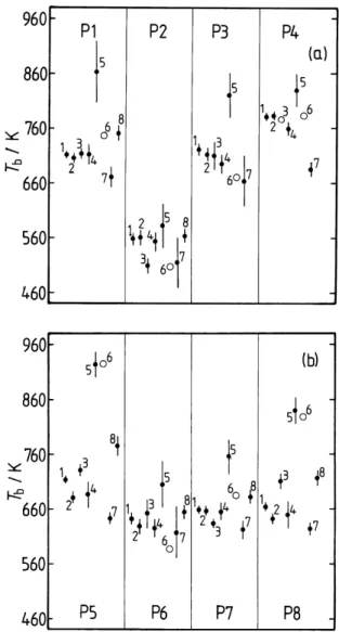
Fig. 1. Boiling points (Tb) of the primary surrogate compounds in
the UCD-CACM model, calculated using the following methods: 1 – Nannoolal et al. (2004); 2 – Cordes and Rarey (2002); 3 – ACD; 4 – Stein and Brown (1994); 5 – Joback and Reid (1987); 6 – Wen and Qiang (2002a, b); 7 – Constantinou and Gani (1994); 8 – Marrero-Morejon and Pardillo-Fondevila (1999). The error bars are the DDBST average absolute deviations for the method and com-pound class to which the surrogate belongs, except for the ACD prediction for which the ACD uncertainty is shown. No DDBST deviations are currently available for predictions shown as open cir-cles.
The thermodynamic properties of even the relatively small number of secondary compounds that have been identified in controlled laboratory experiments (e.g., Yu et al., 1999; Jaoui et al., 2005) have generally not been measured, and must therefore be estimated using structure-based or other methods. In this work, which is a companion paper to that of Clegg et al. (2008), hereafter referred to as Paper 1, we examine uncertainties in predictions of the sub-cooled liquid vapour pressures p◦i that control the gas/aerosol partitioning
of semi-volatile compounds. We also estimate the vapour pressures of the primary surrogate compounds in the UCD-CACM model, which are currently assumed to be involatile, because there is evidence that high molecular weight hydro-carbons and other primary emissions are able to partition be-tween gas and aerosol phases (Fraser et al., 1997, 1998).
At least two approaches are possible: the first is to assess predictive methods against reliable data for compounds of a similar molecular weight and functional group composition to those of the secondary organic aerosol (SOA) compounds likely to occur in the atmosphere. The compounds are in many cases the products of oxidation and are likely to be highly polar, containing multiple –COOH and –OH groups for example. While such a study is now being carried out (M. Barley, personal communication), and see also Camre-don and Aumont (2006), there are very few data for such compounds especially in the sub-cooled liquid state that is thought to apply to atmospheric aerosols. An alternative, complementary, approach which we adopt is to apply cur-rent predictive methods to both the surrogate organic com-pounds in the UCD-CACM model and the reaction products they represent. This enables us (i) to establish approximate ranges of uncertainty of the vapour pressures of compounds present in the model; (ii) to assess the further approximations inherent in grouping multiple compounds into surrogates to which single values of fi and p◦i are applied and, (iii) to
de-termine (in Paper 1) the significance of uncertainties in terms of gas/aerosol partitioning and SOA formation.
The results are relevant, first, to the general development of atmospheric aerosol models based upon an explicit chem-istry and corresponding to Fig. 1 in Paper 1, highlighting par-ticular areas in which a better quantitative understanding of the physical chemistry is needed. Second, they identify el-ements of the UCD-CACM model on which future work is likely to focus.
2 The organic compounds and surrogates
The Caltech Atmospheric Chemistry Mechanism is used to describe the photochemical reactions in the atmosphere in-cluding the formation of semi-volatile products leading to the production of secondary organic aerosol. The mod-elled system consists of 139 gas-phase species participating in 349 chemical reactions, and inorganic ions, gases, and solids (Griffin et al., 2002). For the purpose of calculating gas/aerosol partitioning, the semi-volatile species generated by chemical reaction, and capable of forming SOA, are com-bined into a set of 10 surrogate species A1-5 and B1-5 (Grif-fin et al., 2003). We note that the structure of compound B5 (S10 in Fig. 1 of Griffin et al.) has been corrected as de-scribed by Griffin et al. (2005), and is shown in Fig. 22 of Paper 1. There are, in addition, 8 primary organic hydrocar-bon surrogate compounds (P1-8).
Table 1. Variation of Sub-cooled Liquid Vapour Pressure p◦(atm) at 298.15 K with the Addition of Functional Groups. Hydrocarbon p◦ Alcohol p◦ Carboxylic acid p◦
butane 2.4 1-butanol 8.8E-3 butanoic acid 7.74E-4 2-butanol 2.4E-2 succinic acid 4.21 E-8a 1, 2-butanediol 9.9E-5
1, 4- butanediol 7.5E-6 1, 3- butanediol 4.7E-5 2, 3- butanediol 2.4E-4
Notes: values of p◦were taken from the DIPPR Thermophysical Properties Database. aEstimated for this compound which is primary organic surrogate P2, see Table 5.
3 Vapour pressures
In the UCD-CACM model, subcooled vapour pressures of secondary organic surrogates A1-5 and B1-5 are estimated by the method of Myrdal and Yalkowsky (1997). This uses the boiling temperature at atmospheric pressure (Tb), the
en-tropy of boiling (1Sb), and the heat capacity change upon
boiling (1Cp(gl)). The normal boiling points used in
previ-ous applications of the UCD-CACM model were obtained either from measurements or using the estimation software of Advanced Chemistry Developments (ACD) which is de-scribed in a manuscript by Kolovanov and Petrauskas (un-dated1), (B. L. Hemming, personal communication). Esti-mates of 1Sbare obtained from the molecular structure and
are expressed in terms of the numbers of torsional bonds (τ , Eq. (8) of Myrdal and Yalkowsky) and a hydrogen bonding term HBN (their Eq. 9). Values of τ used previously for some of the SOA surrogate compounds were in error. The correct values of τ and HBN, used in all calculations in this work, are given for the 8 primary and 10 semi-volatile surro-gate compounds in the Appendix. The heat capacity change
1Cp(gl)is expressed as a function of τ (Eq. (11) of Myrdal
and Yalkowsky). The overall accuracy of the method, assum-ing that the boilassum-ing temperature Tb is known, is dependent
upon the accuracy of 1Sb and the assumption that 1Cp(gl)
varies little with temperature. The expressions for 1Sb and
1Cp(gl)were obtained by Myrdal and Yalkowsky by fitting
to experimental data for 297 compounds. From their Fig. 3 it is apparent that only 19 of the compounds have pressures
<10−6atm, 7 below 10−8atm, and 2 below 10−10atm. For experimental vapour pressures less than 10−6atm the resid-uals in the figure correspond to errors ranging from ×2.2 too high, to too low by about a factor of 5.
The accuracy of the method for the polar multifunctional compounds of interest to atmospheric chemists, and repre-sented by surrogates here, is hard to establish due to the lack of data. However, it seems certain to be very much 1Kolovanov, E. and Petrauskas, A.: Towards the maximum ac-curacy for boiling point prediction, undated manuscript.
poorer than the 23% obtained by Myrdal and Yalkowsky with a test data set of compounds not used in their fit, even without taking into account the fact that the boiling tem-peratures have to be estimated here. The test data used by Myrdal and Yalkowsky consisted of a group of 19 com-pounds which, though structurally diverse, are mostly mono-functional. Measured pressures, with one exception, range from 10−1.02 to 10−2.99 atmospheres. These values are or-ders of magnitude greater than those of the semi-volatile compounds of interest in this study. Errors in the vapour pressures predicted by Myrdal and Yalkowsky ranged from 0 to a factor of 2.45 for the test data set.
We note that Zhao et al. (1999) later proposed an alter-native expression for the entropy of boiling, and Sangvi and Yalkowsky (2006a) one for the heat capacity change. Nei-ther have so far been evaluated for the prediction of vapour pressures. Our own tests, using data for multifunctional al-cohols, suggest that the original HBN term of Myrdal and Yalkowsky (1997) is preferable to the equivalent used in Eq. (5) of Zhao et al. (1999) because, first, the hydrogen bonding effect (which acts to lower vapour pressure) is re-duced as molecular mass increases. This is realistic: the ef-fect of an –OH or –COOH group on the vapour pressure of a very large molecule, with many carbon atoms, is less than on a small molecule. Second, the effect of adding further polar groups results in a less than linear increase in the hydrogen bonding influence on the predicted entropy of boiling.
The effect of molecular structure and functional group composition on vapour pressure is very important. Table 1 lists vapour pressures for butane and related C4alcohols and carboxylic acids. The addition of first one, and then two polar functional groups to the butane molecule results in a lowering of p◦by orders of magnitude. The positions of the groups on the molecule make a large difference, by more than an order of magnitude in some of the examples shown.
In this work we compare estimates of subcooled liquid vapour pressures p◦and enthalpies of vaporisation 1Hovapfor the semi-volatile surrogate compounds using: (i) the Myrdal and Yalkowsky (1997) method combined with a range of current techniques for predicting the boiling points Tb, (ii)
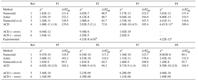
Table 2. Estimated Boiling Temperatures Tb(K), at Atmospheric Pressure, of the Primary Hydrocarbon Surrogates.
Method Ref. P1 P2 P3 P4 P5 P6 P7 P8
Nannoolal et al. 1 712.0 559.4 721.5 780.8 713.0 641.3 657.8 664.2 Cordes and Rarey 2 705.7 560.8 712.0 783.1 680.7 627.4 655.5 641.8
ACD 3 714.1 509.3 710.3 774.1a 730.6 651.4 632.6 709.7
Stein and Brown 4 (712.0) 553.6 695.4 (759.5) (685.5) 624.5 655.2 (648.8) Joback and Reid 5 [863.1] 582.1 820.8 (829.1) [922.7] 705.3 757.0 [839.2] Wen and Qiang 6 [746.5] 507.1 670.4 [782.7] [924.6] 585.6 683.4 [826.6] Constantinou and Gani 7 (671.1) 515.1 663.4 685.2 642.4 616.2 621.6 623.9
Marrero-Morejon 8 (751.1) 564.2 – – 773.8 653.7 681.0 715.5
Other 591b – – – – – – –
ACD (+/–) 3 8 13 25 – 12 25 5 12
Notes: the structures of the molecules are as listed in Fig. 1 of Griffin et al. (2003), with the exception of P5, for which the structure given by Chemical Abstracts for hopane (C30H52, registry number 471-62-5) was used. Values in square brackets [ ] are predictions using methods that are “unrecommended”, for the compound class to which the surrogate belongs, by the program Artist (DDBST Software and Separation Technology GmbH, 2005) which was used to generate the predictions. Values in parentheses ( ) are similarly listed as “unreliable”, and “– ” indicates that the calculation could not be carried out, for example because of the presence of groups in the molecule whose properties are undefined. The bottom row lists uncertainties (K) associated with the ACD prediction. a Experimental. bDIPPR Thermophysical Properties Database, predicted by staff with a probable error of <25%. References: 1 – Nannoolal et al. (2004); 2 – Cordes and Rarey (2002); 3 – Kolovanov and Petrauskas (undated), and ACDLabs software v8.0 (Advanced Chemistry Development Inc., 2004); 4 – Stein and Brown (1994); 5 – Joback and Reid (1987); 6 – Wen and Qiang (2002a, b); 7 – Constantinou and Gani (1994); 8 - Marrero-Morejon and Pardillo-Fontdevila (1999).
the UNIFAC-based method of Asher and Pankow (2006) and Asher et al. (2002), and (iii) the approach of Nannoolal (2007) which is an extension of the boiling point method of Nannoolal et al. (2004). The 8 primary hydrocarbons in the UCD-CACM model (which are currently assumed to be in-volatile) are included in these comparisons. Vapour pressures calculated for the 38 semi-volatile compounds assigned to the semi-volatile surrogates in the UCD-CACM model are also compared to those for the surrogates themselves. Fi-nally, the effects of uncertainties in the values of p◦of water-soluble compounds are examined using simple partitioning calculations for a range of atmospheric liquid water contents. 3.1 Estimation of normal boiling points
The boiling points of all the surrogate compounds are un-known, with the exception of primary hydrocarbon surro-gate P4. Most values used in the UCD-CACM model to date have been estimated using the ACD software package ACDLabs 8.0. Here we compare boiling temperatures Tb
es-timated using eight selected predictive methods, whose char-acteristics and claimed accuracy are summarised in the Ap-pendix (Nannoolal et al., 2004; Cordes and Rarey, 2002; Wen and Qiang, 2002a, b; Marrero-Morejon and Pardillo-Fontdevila, 1999; Stein and Brown, 1994; Constantinou and Gani, 1994; Joback and Reid, 1987; Advanced Chemistry Developments (Kolovanov and Petrauskas, undated)). The methods are based upon molecular structure. With the excep-tion of the ACD method, all calculaexcep-tions have been carried
out using software available from DDBST Software and Sep-aration Technology GmbH. This also provides summaries of the accuracies of the methods, based upon comparisons with all the available normal boiling points in the Dortmund Data Bank. Note that no values are yet available for the method of Wen and Qiang (2002a, b). These summaries are presented as average absolute deviations in Tb for each class of
com-pounds (defined in terms of the functional group(s) and types of bonds present) to which the compound of interest belongs. Many molecules, including those considered here, fall into several classes. In these cases we follow the DDBST rec-ommendation and take the largest error listed as being repre-sentative, but recognise that for multifunctional compounds the errors for each class to which the compound belongs are likely to be additive to some degree. The ACD method pro-vides an error estimate with each predicted Tbvalue. It is not
clear how this is obtained.
Some general comments regarding the boiling point meth-ods can be made: first, the linear relationship employed by Joback and Reid (1987) between the sum of group contri-butions and boiling point is only valid over a limited range of molecular size – e.g., for molecules with up to about 8 –CH2– groups in the case of linear alkanes, and up to 15
−CH2− groups for n-alkanols (Cordes and Rarey, 2002). Second, the effect of polar functional groups such as –OH and –COOH on boiling point is not simply additive, as is of-ten assumed in group contribution methods. Of those meth-ods considered here, those of Joback and Reid (1987), Stein
and Brown (1994), and Wen and Qiang (2002a, b) are es-sentially additive, whereas that of Constantinou and Gani (1994) is logarithmic, and the method of Marrero-Morejon and Pardillo-Fontdevila (1999) has a dependency on molec-ular mass. In the equations of Cordes and Rarey (2002) and Nannoolal et al. (2004) the sum of group contributions is di-vided by a term in the number of atoms in the molecule. The ACD method appears to differ from the others in that predic-tions use a combination of internal database of boiling points and a structure/fragmentation algorithm.
Estimated boiling points for the primary hydrocarbons are listed in Table 2, and shown in Fig. 1. Many of the estimates of Tbdisagree by more than would be expected from the
av-erage absolute deviations (provided by the DDBST software, as noted above) which are also shown.
The ACD predictions, and those of the methods of Cordes and Rarey (2002) and of Nannoolal et al. (2004), agree within the quoted uncertainties of the methods for surrogates P1, P3, P4 and P6. The earliest method, that of Joback and Reid (1987), yields much higher Tbthan the other methods in
al-most all cases. For many of the molecules this is due to the method’s known limitations with respect to molecular size, noted above. Values from the method of Wen and Qiang (2002a, b) are also very high for P5 and P8. Excluding the predictions from these two methods, quite large differences are also found for succinic acid (P2) and for poly-substituted decalin (P8). For succinic acid this is not surprising, as these and other prediction methods are generally least satisfactory for multifunctional compounds, particularly those which are small – for which the functional groups are likely to have the greatest influence on physical properties – or for molecules in which the groups are close enough to interact with one another. The vapour pressure p◦of P2 (which is
represen-tative of dicarboxylic acids in the aerosol) can be estimated independently of the boiling points (see below), and the re-sult suggests that the true boiling point probably lies about midway between the two predictions. In the UCD-CACM model P8 represents a range of involatile hydrocarbon mate-rial found in aerosols, the composition of which is not well understood. The fact that this compound has a boiling point, and an estimated vapour pressure, similar to a number of the other compounds here suggests that the structure chosen for P8 may need to be reconsidered.
If the predictions of the Joback and Reid (1987) method, all values for P8, and a few individual estimates (P5 – Marrero-Morejon and Pardillo-Fontdevila; P4 – Constanti-nou and Gani) are ignored then most values of Tbin Table 2
fall within a range of about 75 K or less. The methods that agree most closely are those of Nannoolal et al. (2004), ACD, and Stein and Brown (1994). (The method of Nannoolal et al. (2004) is a further development of that of Cordes and Rarey (2002), and the two give similar predictions.)
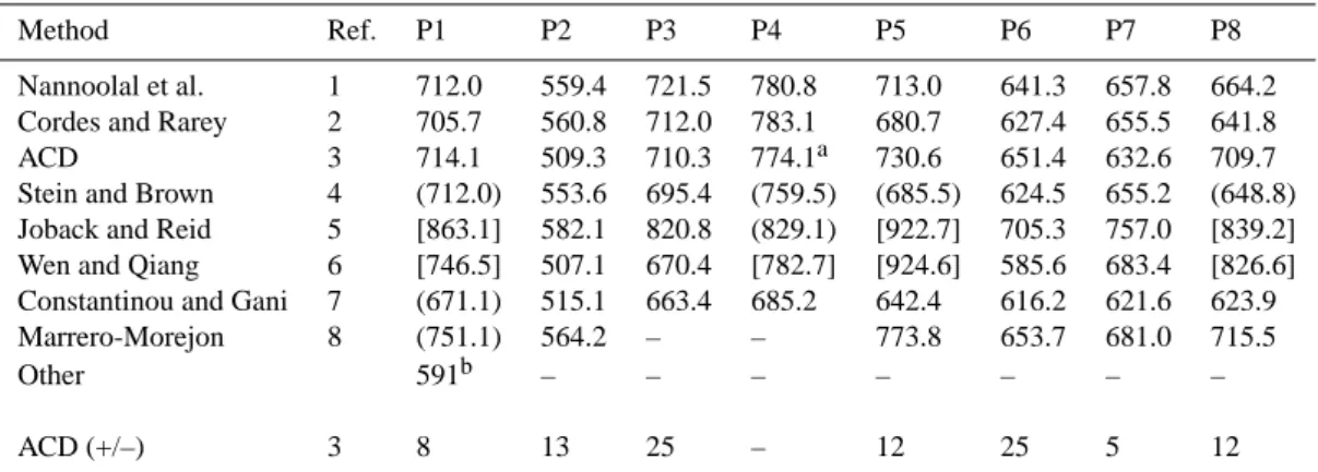
Estimated boiling points for the A and B surrogate com-pounds, including the values used in the UCD-CACM model code, are shown in Table 3 and in Fig. 2. It is not possible
Fig. 2. Boiling points (Tb) of the semi-volatile surrogate
com-pounds in the UCD-CACM model, calculated using the follow-ing methods: 1 – Nannoolal et al. (2004); 2 – Cordes and Rarey (2002); 3 – ACD; 4 – Stein and Brown (1994); 5 – Joback and Reid (1987); 6 – Wen and Qiang (2002a, b); 7 – Constantinou and Gani (1994); 8 – Marrero-Morejon and Pardillo-Fondevila (1999). The error bars are the DDBST average absolute deviations for the method and compound class to which the surrogate belongs, except for the ACD prediction for which the ACD uncertainty is shown. No DDBST deviations are currently available for predictions shown as open circles.
to calculate Tbfor some compounds using some of the
meth-ods, notably B3-5 which contain the group –O–NO2. Nor are DDBST error estimates available for all compounds. The uncertainties associated with the ACD predictive method are significantly greater for these compounds than for the pri-mary surrogates. However, except for A1, A4 and B3 the ACD predictions for the semi-volatile compounds are still consistent with those using the Nannoolal et al. and Stein
Table 3. Estimated Boiling Temperatures Tb(K), at Atmospheric Pressure, of the Biogenic and Anthropogenic Surrogate Compounds.
Method Ref. A1 A2 A3 A4 A5 B1 B2 B3 B4 B5
Nannoolal et al. 1 529.6 639.5 – 598.9 553.6 651.1 614.4 603.5 641.3 546.5 Cordes and Rarey 2 530.5 641.5 553.6 600.8 564.7 661.4 611.5 601.0 638.8 546.5
ACD 3 638.2 683.0 560.4 664.3 599.5 681.3 623.0 641.5 669.2 564.4
Stein and Brown 4 520.1 636.7 544.6 596.3 551.9 655.8 605.8 – – –
Joback and Reid 5 536.4 730.4 580.1 700.2 621.8 825.1 664.2 – – –
Wen and Qiang 6 425.9 610.5 478.8 621.5 437.4 556.2 496.4 – – –
Constantinou and Gani 7 – 598.4 547.1 – 551.6 647.6 599.3 – – –
Marrero-Morejon 8 – – – – 588.5 – 641.2 – – –
UCD-CACM model 560 698 575 679 615 685.3 634 645.5 672.5 566.3
Other 569a
ACD (+/–) 3 25 35 40 42 32 45 30 21 25 29
Notes: the structures of the molecules are as listed in Fig. 1 of Griffin et al. (2003), (A1-5 correspond to S1-5, and B1-5 to S6-10), with the exception of B5 (S10) which has been corrected to the structure given in Appendix A of Clegg et al. (2008). Dashes “–” indicate that the calculation could not be carried out, for example because of the presence of groups in the molecule whose properties are undefined. The bottom row lists uncertainties (K) associated with predictions by the ACD method.aDIPPR Thermophysical Properties Database, predicted by staff with a probable error of <25%. The numbered references are the same as in Table 2.
Table 4. The Effect of Errors in the Boiling Temperature Tb(K) on
Estimated Vapor Pressures at 298.15 K for Compounds with Nor-mal Boiling Points from 500 K to 800 K.
Tberror p◦/p◦(base) (500 K) (600 K) (700 K) (800 K) –75 56.8 70.5 88.8 105. –50 14.1 17.5 20.2 22.6 –20 2.93 3.17 3.36 3.50 –10 1.72 1.78 1.83 1.87 0 1.0 1.0 1.0 1.0 10 0.580 0.559 0.544 0.533 20 0.335 0.311 0.295 0.284 50 0.063 0.0529 0.0466 0.0423 75 0.015 0.0118 0.0099 0.0086 Notes: p◦(base) is the vapour pressure calculated at the listed boil-ing point usboil-ing the Myrdal and Yalkowsky (1997) equation, and p◦ is the value of the vapour pressure calculated for the listed boiling point + Tberror. Thus, for example, an estimate of Tbthat is 75 K
too low for a compound with a true boiling point of 500 K will yield a vapour pressure that is too high by a factor of 56.8.
and Brown methods. For surrogates A1, A2, A4, A5 and B3 the values of Tbobtained using the ACD method, and that of
Nannoolal et al., differ by amounts ranging from 9 K to over 100 K with the ACD predictions always higher.
The general influence of errors in the predicted Tbon
cal-culations of p◦at 298.15 K using the Myrdal and Yalkowsky (1987) equation is illustrated in Table 4. This lists the ratio of the predicted p◦to the base p◦(i.e., the value calculated using the Myrdal and Yalkowsky equation for the Tbabove
each column) for assumed errors in Tbranging from –75 K
to +75 K. It can be seen that there is a dependence of the ratio on Tbfor large errors. Variations in predicted Tbover
ranges of 20 K to 50 K are typical for both primary and semi-volatile surrogate compounds, even ignoring the predicted Tb
that deviate most. The error estimates for the ACD predic-tions range from ±5 K to ±45 K, see Tables 2 and 3, and while they are the most conservative they also appear to be the most realistic. The results in Table 4 show that these uncertainties are likely to result in calculated p◦ which are incorrect by factors of about ×1.4 to ×20, without taking into account additional errors associated with the use of the Myrdal and Yalkowsky equation. It will be seen in the fol-lowing section that values of p◦based on Tbestimated by the
methods considered here do indeed differ by similar or larger factors.
3.2 Predicted vapour pressures
Estimated pure compound vapour pressures at 298.15 K for surrogate primary compounds P1 to P8 are shown in Table 5. The methods used are the Myrdal and Yalkowsky model with boiling points from Nannoolal et al. (2004), ACD including values based upon the upper and lower uncertainty limits of the predicted Tb, the UNIFAC based method of Asher and
co-workers, and a recently completed extension of the boil-ing point method of Nannoolal et al. (2004) to predict p◦. All compounds have vapour pressures below the lower limit of validity of the ACD vapour pressure prediction model (0.001 mm Hg) in the ACDLabs software, and therefore that method is not used.
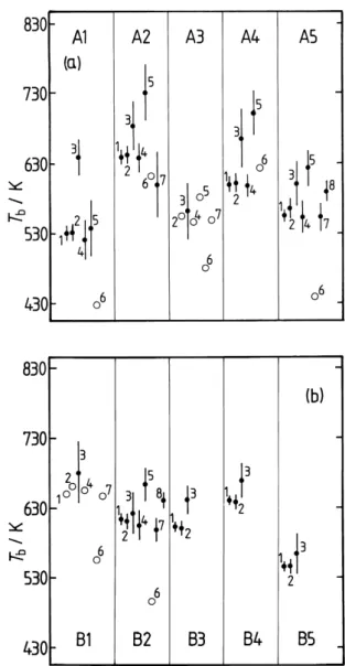
Table 5. Estimated Vapour Pressures p◦(atm) and Enthalpies of Vaporisation 1Hvapo (kJ mol−1) of Primary Hydrocarbon Surrogate Species
as Supercooled Liquids at 298.15 K.
Ref. P1 P2 P3 P4
Method p◦ 1Hvapo p◦ 1Hvapo p◦ 1Hvapo p◦ 1Hvapo
Nannoolal 1 1.82E-11 131.6 4.65E-7 88.5 3.17E-13 152.5 3.61E-12 137.4
Asher 2 2.55E-15 232.2 8.12E-8 88.7 9.04E-16 194.9 8.00E-13 154.5
Nannoolal et al. 3 1.26E-11 128.5 1.08E-6 82.7 2.33E-10 107.5 4.41E-11 110.6 ACD 4 1.08E-11 (1.8) 129.0 2.03E-5 (2.1) 72.8 4.56E-10 (4.5) 105.4 6.45 E-11a 109.4
ACD (+ error) 5 6.04E-12 9.58E-6 1.02E-10 –
ACD (− error) 6 1.94E-11 4.29E-5 2.02E-9 –
Experimental 4.21E-8 (4.0)b 4.22E-12c
Ref. P5 P6 P7 P8
Method p◦ 1Hvapo p◦ 1Hvapo p◦ 1Hvapo p◦ 1Hvapo
Nannoolal 1 9.47E-10 110.5 6.54E-10 117.2 1.56E-10 123.7 8.063E-8 89.1
Asher 2 2.60E-12 182.2 4.23E-10 118.5 1.31E-11 170.4 2.45E-10 132.5
Nannoolal et al. 3 1.83E-9 99.2 1.81E-8 94.3 1.66E-9 108.0 1.20E-8 95.7 ACD 4 6.82E-10 (2.0) 102.4 9.98E-9 (4.5) 96.2 8.71E-9 (1.4) 102.5 8.30E-10 (2.0) 104.5
ACD (+ error) 5 3.46E-10 2.23E-09 6.28E-09 4.06E-10
ACD (− error) 6 1.34E-09 4.39E-08 1.21E-08 1.69E-09
Notes: numbers in parentheses following the ACD p◦are the factors by which p◦is increased and decreased if the upper and lower bounds on the estimated Tbare assumed. aBased on an experimental boiling point from an unknown source, quoted by the ACD software, hence
there is no error estimated. bBased on the vapour pressure of the solid acid, its aquous solubility and activity coefficient calculated using UNIFAC, but using modified parameters presented by Peng et al. (2001). The value in parentheses is the factor by which the estimated vapor pressure is altered if standard UNIFAC parameters are used.cLei et al. (2002). References: 1 – Nannoolal (2007) (the method is based upon that of Nannoolal et al. (2004) for Tb); 2 – Asher and Pankow (2006), and Asher et al. (2002); 3 – Myrdal and Yalkowsky (1997) equation,
with Tbfrom Nannoolal et al. (2004); 4 – Myrdal and Yalkowsky (1997) equation, with Tbcalculated using the ACD software; 5 – as for
4, except that the uncertainty ACD (+/–) from Table 2 is added to Tb; 6 – as for 4, except that the uncertainty ACD (+/–) from Table 2 is
subtracted from Tb.
We have included in Table 5 a value of p◦for succinic acid (P2) derived from the vapour pressure of the solid (Ribeiro da Silva et al., 2001), its activity product in water (see Clegg and Seinfeld, 2006) and estimates of its activity coefficient from UNIFAC. For P4 an experimental value based upon gas chro-matographic retention time was obtained (Lei et al., 2002). Upper and lower limits for p◦, based upon the uncertainty in the ACD estimate of Tb, are listed in the table and are also
expressed in terms of an error factor in parentheses. Thus the Myrdal and Yalkowsky equation, using the ACD Tb=714.1 K
for P1, yields a p◦of 1.08×10⁻¹¹ atm for the supercooled liquid at 298.15 K. Adding the uncertainty limit of ±8 K (Ta-ble 2), to obtain Tb=722.1 K and Tb=706.1 K, yields p◦
val-ues that differ by a factor of 1.8 from the base prediction. The Nannoolal (2007) vapour pressure model, and the Myrdal and Yalkowsky method with the ACD and Nannoolal et al. (2004) estimates of Tb, agree best for hydrocarbons P1,
P5 and P8. In most cases the predictions of the UNIFAC-based approach are lower, in some instances by orders of magnitude. For P4 the experimentally determined vapour pressure agrees fairly closely with the result from the Nan-noolal vapour pressure model, and to within an order of mag-nitude with the Myrdal and Yalkowsky prediction based upon the experimental boiling point.
The value of p◦estimated for succinic acid (P2) from the solubility of the solid in water and its vapour pressure (see Table 5) is lower than all the other values except that from the model of Asher (Asher and Pankow, 2006). This acid was included in the data set they used for fitting their model. We also note that the Myrdal and Yalkowsky method, using an estimated Tb of 591 K from the DIPPR Thermophysical
Properties Database, yields p◦ equal to 1.61×10⁻⁷ atm at 298.15 K. This agrees reasonably well with the value based upon the vapour pressure of the solid. It is unclear which of the many estimates of p◦is more nearly correct.
Estimated p◦and values of 1Hvapo for the surrogate com-pounds treated as semi-volatile in the UCD-CACM model are shown in Tables 6 and 7. For oxalic acid (A1) there is also an estimate based upon the Henry’s law constant (Clegg et al., 1996), and a further value based on a predicted Tbtaken
from the DIPPR Thermophysical Properties Database. The vapour pressures, with the exception of the prediction based upon the ACD boiling point, range between about 2×10⁻⁷ to 5×10⁻⁶atm and agree reasonably well. Previous work has suggested that oxalic acid will partition in the atmo-sphere such that significant amounts can occur in both the aerosol and gas phases, dependent upon atmospheric condi-tions (Clegg et al., 1996). The UNIFAC-based method is
Table 6. Estimated Vapour Pressures of Vapour Pressures p◦(atm) and Enthalpies of Vaporisation 1Hvapo (kJ mol−1) of Semi-Volatile
Surrogate Species as Supercooled Liquids at 298.15 K.
A1 A2 A3 A4 A5
Method Ref. p◦ 1Hvapo p◦ 1Hvapo p◦ 1Hvapo p◦ 1Hvapo p◦ 1Hvapo
UCD-CACM model
7.34E-7 84.2 5.02E-10 106.4 1.01E-6 81.3 1.50E-9 103.2 8.19E-8 90.7
Nannoolal 1 6.37E-6 76.3 2.81E-10 122.1 – – 1.12E-8 105.6 1.38E-6 82.6
Asher 2 2.87E-7 73.0 4.47E-11 140.5 1.64E-7 116.9 1.15E-8 115.0 1.51E-6 106.3
Nannoolal et al. 3 4.56E-6 78.2 1.76E-8 95.1 – – 1.87E-7 87.6 2.95E-6 78.6
ACD 4 5.80E-9 (4.9) 1.26E-9 (8.6) 2.32E6 (9.9) 3.69E-9 (13.2) 100.4 2.05E-7 (6.7) 87.6
ACD (+ error) 5 1.19E-9 104.7 1.05E-8 96.8 2.16E-5 70.9 4.66E-8 92.2 1.33E-6 81.3
ACD (– error) 6 2.78E-8 94.8 1.46E-10 110.3 2.35E-7 86.1 2.79E-10 108.5 3.06E-8 93.9
DIPPR 7 4.25E-7 86.0
Other 2.62E-7a 78.9 3.47E-6 77.2b
Notes: numbers in parentheses following ACD p◦are the factors by which p◦is increased and decreased if the upper and lower bounds on the estimated Tbare assumed.aBased on a Henry’s law constant from Clegg et al. (1996), and UNIFAC using modified values of parameters
determined by Peng et al. (2001). Alternatively, p◦=7.67×10⁻⁸ atm is obtained assuming Raoult’s law behavior of the undissociated molecule, and 6.53×10⁻⁸atm using UNIFAC with unmodified parameters to calculate the activity coefficient of the acid. Dissociation is taken into account in these calculations. bMyrdal and Yalkowsky (1997) equation, with Tbfrom Cordes and Rarey (2002). References:
1 – Nannoolal (2007); 2 – Asher and Pankow (2006), and Asher et al. (2002); 3 – Myrdal and Yalkowsky (1997) equation, with Tbfrom
Nannoolal et al. (2004); 4 – Myrdal and Yalkowsky (1997) equation, with Tbcalculated using the ACD software; 5 – as for 4, except that the
uncertainty ACD (+/–) from Table 3 is added to Tb; 6 – as for 4, except that the uncertainty ACD (+/–) from Table 3 is subtracted from Tb; 7 – Mydral and Yalkowsy (1997) equation, with Tbfrom the DIPPR Thermophysical Database.
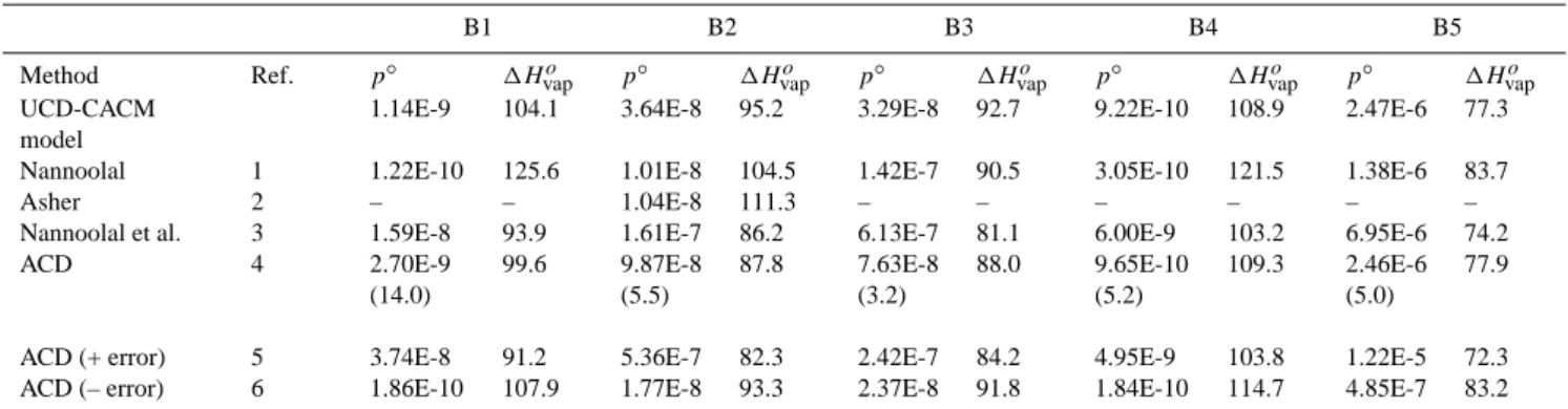
Table 7. Estimated Vapor Pressures of Vapor Pressures p◦(atm) and Enthalpies of Vaporisation 1Hvapo (kJ mol−1) of Semi-Volatile
Surro-gate Species as Supercooled Liquids at 298.15 K.
B1 B2 B3 B4 B5
Method Ref. p◦ 1Hvapo p◦ 1Hvapo p◦ 1Hvapo p◦ 1Hvapo p◦ 1Hvapo
UCD-CACM model
1.14E-9 104.1 3.64E-8 95.2 3.29E-8 92.7 9.22E-10 108.9 2.47E-6 77.3
Nannoolal 1 1.22E-10 125.6 1.01E-8 104.5 1.42E-7 90.5 3.05E-10 121.5 1.38E-6 83.7
Asher 2 – – 1.04E-8 111.3 – – – – – –
Nannoolal et al. 3 1.59E-8 93.9 1.61E-7 86.2 6.13E-7 81.1 6.00E-9 103.2 6.95E-6 74.2
ACD 4 2.70E-9 (14.0) 99.6 9.87E-8 (5.5) 87.8 7.63E-8 (3.2) 88.0 9.65E-10 (5.2) 109.3 2.46E-6 (5.0) 77.9
ACD (+ error) 5 3.74E-8 91.2 5.36E-7 82.3 2.42E-7 84.2 4.95E-9 103.8 1.22E-5 72.3
ACD (– error) 6 1.86E-10 107.9 1.77E-8 93.3 2.37E-8 91.8 1.84E-10 114.7 4.85E-7 83.2
Notes: numbers in parentheses following the ACD p◦are the factors by which p◦is increased and decreased if the upper and lower bounds on the estimated Tbare assumed. References: 1 – Nannoolal (2007); 2 – Asher and Pankow (2006), and Asher et al. (2002); 3 – Myrdal and Yalkowsky (1997) equation, with Tbfrom Nannoolal et al. (2004); 4 – Myrdal and Yalkowsky (1997) equation, with Tbcalculated using the
ACD software; 5 – as for 4, except that the uncertainty ACD (+ error) from Table 3 is added to Tb; 6 – as for 4, except that the uncertainty
ACD (– error) from Table 3 is subtracted from Tb.
not applicable to most of surrogates B1-5 because not all of the required structural groups are defined. It also yields en-thalpies of vaporization that are consistently greater than the other approaches.
Camredon and Aumont (2006) have assessed four structure-activity relationships for estimating p◦ against a database of experimental values. The methods assessed in-clude both the UNIFAC-based approach of Asher and co-workers, and also the Myrdal and Yalkowsky (1997) equation combined with the boiling point equation of Joback and Reid (1987) which we have found yields significantly higher Tb
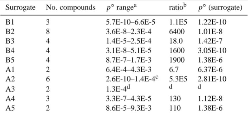
Table 8. Subcooled Liquid Vapour Pressures p◦(atm) of the Component Compounds of the Semi-Volatile Surrogate Species at 298.15 K.
Surrogate No. compounds p◦rangea ratiob p◦(surrogate)
B1 3 5.7E-10–6.6E-5 1.1E5 1.22E-10
B2 8 3.6E-8–2.3E-4 6400 1.01E-8
B3 4 1.4E-5–2.5E-4 18.0 1.42E-7
B4 4 3.1E-8–5.1E-5 1600 3.05E-10
B5 4 8.7E-7–1.7E-3 1900 1.38E-6
A1 2 6.4E-4–4.3E-3 6.7 6.37E-6
A2 6 2.6E-10–1.4E-4c 5.3E5 2.81E-10
A3 2 1.3E-4d d d
A4 3 3.3E-7–4.3E-5 130 1.12E-8
A5 2 8.6E-5–9.3E-3 110 1.38E-6
Notes: the method of Nannoolal (2007) was used to calculate the results above. The assignment of reaction products to surrogate species in the UCD-CACM model is as follows: B1=AP1+AP6+UR31; B2=ADAC+RPR7+RP14+RP19+UR2+UR14+UR27+ARAC; B3=AP10+UR11+UR15+UR19; B4=AP11+AP12+UR20+UR34; B5=AP7+AP8+UR5+UR6; A1=UR21+UR28; A2=RP13+RP17+RP18+UR26+UR29+UR30; A3=RPR9+RP12; A4=UR3+UR8+UR23; A5=UR7+UR17, see Griffin et al. (2002). aThe largest and smallest vapour pressures of the components assigned to the surrogate species.bThe value of the largest vapour pressure in the previous column, divided by the smallest.cVapour pressures of components RP17 and UR29 cannot be calculated using this method. dThe vapour pressure RPR9 cannot be calculated using this method.
than other methods (Figs. 1 and 2). Camredon and Aumont conclude that these two methods of estimating p◦were the most reliable for compounds with low vapour pressures, al-though they also found that values of p◦predicted using the
different methods could vary by factors of greater than 100. These findings are broadly consistent with our results, al-though our calculations and the work of Stein and Brown (1994) suggests that the equation of Joback and Reid does not yield the most accurate predictions of Tb. This is also
noted by Camredon and Aumont, who did not use the work of Stein and Brown as it was based upon many of the same data used in their assessment.
The range of vapour pressures obtained by the different methods, and shown in Tables 5 to 7, exceed by a significant margin what would be expected from the uncertainties asso-ciated with each boiling point estimation and vapour pres-sure prediction method. This must be due partly to the fact that the models are fitted to data for generally much sim-pler molecules than those of interest here, which also have higher vapour pressures (lower boiling points). The ranges of the calculated vapour pressures in the tables, as ratios
p◦(highest)/p◦(lowest), are: 7.1×10³ [1.7] (P1), 482 [44] (P2), 5.0×10⁵[1.4×10³] (P3), 80 [18] (P4), 704 [2.7] (P5), 43 [43] (P6), 665 [56] (P7), 329 [329] (P8), 1098 [1098] (A1), 393 [63] (A2), 21 [2.3] (A3), 125 [125] (A4), 36 [36] (A5), 130 [–] (B1), 16 [16] (B2), 19 [–] (B3), 20 [–] (B4) and 5.0 [–] (B5). The values in square brackets are ratios which omit predictions of the UNIFAC-based method of Asher, and are in many cases smaller. However, it is unclear whether the greater consistency of the predictions of the other methods is because of higher accuracy or because of their similar-ity (being based upon boiling points). The ranges of
pre-dicted vapour pressures obtained using the various methods are comparable for both primary and secondary compounds, if the UNIFAC-based predictions are omitted, although the uncertainties yielded by the ACD method (and listed in the tables) are lower for the primary compounds P1–P8 as would be expected.
The use of surrogate compounds allows gas/aerosol parti-tioning of the potentially large number of semi-volatile prod-ucts of gas phase reactions to be handled efficiently in at-mospheric calculations. However, key properties – including vapour pressure – of the individual compounds making up each surrogate can also be evaluated, and should probably be used in their assignment. Table 8 summarises the results of vapour pressure predictions for the 38 semi-volatile reac-tion products that make up surrogate compounds A1-5 and B1-5 in the UCD-CACM model, expressed as the range of calculated partial pressures of the component compounds as-signed to each surrogate, and the estimated vapour pressures of the surrogates themselves. The ranges vary from about a factor of 10 (i.e., the highest component vapour pressure di-vided by the smallest) to as much as 105. For some of the surrogate compounds the estimated vapour pressures lie out-side the ranges of p◦of the component compounds, for the method used in the calculations. This is clearly an important problem, and the assignment of surrogate species and their properties needs to be considered carefully in the develop-ment of atmospheric models. It may be best to assign the
p◦of the surrogate species based simply upon averages of
the estimates for the component compounds, giving weight to those that are atmospherically most important.
Based on above comparisons, the vapour pressures of the semi-volatile surrogate compounds are uncertain by an order
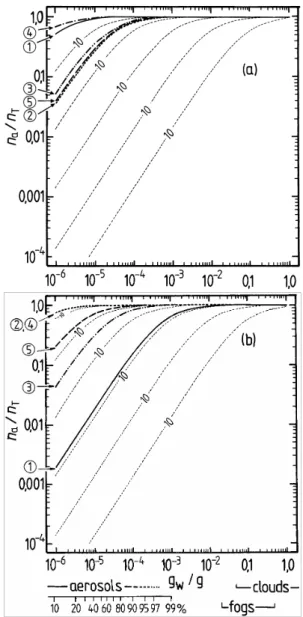
Fig. 3. Fractions of the semi-volatile surrogate compounds present
in the aerosol phase, calculated using Eq. (2a), plotted against atmo-spheric liquid water content (gw/g m−3) for T =298.15 K. Solubility
in water and unit activity coefficients are assumed, and the values of
p◦i are those used in the UCD-CACM model, including the down-ward adjustments to account for the effects of chemical reactions. The thin dashed lines represent the calculated partitioning at inter-vals of factors of 10 in fip◦i. (a) Lines – surrogate species B1-5,
indicated by the circled numbers on the y-axis; (b) lines – surro-gate species A1-5. Approximate ranges of atmospheric liquid water content associated with clouds, fogs and aerosols (including typical RH based on 10−4g m−3of aerosol water at 90% RH, and an acid ammonium sulphate aerosol) are indicated.
of magnitude or greater in most cases. Vapour pressures are very sensitive to the types, numbers, and positions of the functional groups present. Consequently, the estimated vapour pressures of the compounds making up the surrogates
cover very wide ranges, as shown in Table 8. In the UCD-CACM model the vapour pressures of several surrogate com-pounds have been adjusted, based upon chamber measure-ments of SOA formation as described by Griffin et al. (2005). This is likely to be necessary for other atmospheric models of the same type, given that predictive methods for vapour pressures of polar multifunctional compounds yield values that are subject to very large uncertainties, made greater by the need to group compounds into surrogates.
3.3 Effects on partitioning
The impact of uncertainties in the vapour pressures on gas/aerosol partitioning depends on a number of factors: the activity coefficients of the organic species in the aerosol liq-uid phase (since pi=xi fipoi), the total amounts of the
or-ganic compounds per m3 of atmosphere, and the amounts of water (for the water-soluble organics) or primary organic material into which the semi-volatile compounds may parti-tion. The principal water soluble surrogate compounds in the UCD-CACM model are A1-5 and B1-2 (see Paper 1), which we attribute to the presence of polar groups –COOH and – OH. We have investigated the effects of uncertainties in p◦ for these compounds by calculating their equilibrium parti-tioning, at 25◦C, into aerosol and cloud droplets with liquid water contents ranging from 1×10⁻⁶to 1.0 grams of liquid water per m3 of atmosphere. Starting from the equilibrium relationship above, we can write:
ng=xifip◦i(273.15/T )(1/0.022414) (1a)
= [na/(gw/Mw+na)]fip◦i(273.15/T )(1/0.022414) (1b)
where ngis the number of moles of gas i in the vapour phase
at equilibrium, nais the number of moles of i in the aerosol
phase, gw(g m−3) is the amount of liquid water in the aerosol
phase, Mw(18.0152 g mol−1) is the molar mass of water, T
(K) is the ambient temperature and 0.022414 m3mol−1is the molar volume of an ideal gas at standard temperature and pressure (273.15 K). Equation (1b) was solved to obtain na
and ngfor fixed total amounts of organic solute (nT, equal to
na+ng). For the case where the amount of organic solute in
the aerosol, na, is much less than gw/Mw, then the following
equation for the partitioning can be written:
na/nT=1/[1+(Mw/gw)fip◦i(273.15/T )(1/0.022414)](2a)
=1/[1 + 803.75fi(pi◦/gw)(273.15/T )] (2b)
where na/nT is the fraction of the total amount of organic
material per m3 that is present in the aerosol or cloud droplet liquid phase at equilibrium. In these calculations we have used the total amounts (nT) of each compound
listed in Table 1 of Griffin et al. (2003). Values range from 0.1 µg m−3 (4.6×10⁻¹⁰mol m−3) for B5, to 5.5 µg m−3
(1.8×10⁻⁸mol m−3) for B4, and in most cases the
approxi-mate Eqs. (2a, b) apply even at low RH (the smallest values of gw/Mw).
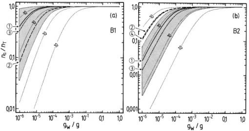
Fig. 4. Fractions of the water-soluble semi-volatile surrogate compounds B1 and B2 present in the aerosol phase at 298.15 K, calculated
using Eq. (2a) for different estimates of p◦i, and plotted against atmospheric liquid water content gw(g m−3). Unit activity coefficients are
assumed. The thin dashed lines represent the calculated partitioning at intervals of factors of 10 in fipi◦. Vapour pressure estimates, Table 7,
were obtained using the equation of Myrdal and Yalkowsky (1997) together with boiling points estimated by the following methods: 1 – value used in UCD-CACM model, without adjustment (solid line); 2 – Nannoolal et al. (2004) (dashed line); 3 – ACD software (dotted line); 4 – a direct prediction of vapour pressure using the method of Asher (Asher and Pankow, 2006; Asher et al., 2002) (dash-dot line). The shaded area corresponds to vapour pressures calculated using the ACD boiling point, plus/minus its estimated uncertainty which is listed in Table 3. (a) Surrogate compound B1; (b) surrogate compound B2.
The results of the partitioning calculations are shown in Fig. 3 for the water soluble surrogate compounds, based upon the adjusted vapour pressures used in the UCD-CACM model. Below the x-axis of plot (b) the amounts of liquid water that are typical of aerosols, clouds, and fogs are indi-cated. In the aerosol region, (gw<1×10⁻⁴g H2O m−3), the equivalent RH above an acid ammonium sulphate aerosol is marked, based upon a rough 1×10⁻⁴g m−3of liquid water for an urban environment at 90% RH. The partitioning cal-culations were carried out assuming fi=1.0 (Raoult’s law).
However, the results of other calculations of fi using
UNI-FAC which are discussed in Paper 1 suggest that actual val-ues are much greater than this, in some cases by orders of magnitude. (Recall that these activity coefficients are for a reference state of the pure subcooled organic compound. Consequently values for dilute solutions in water are gener-ally very different from unity.) The contours on each graph represent the calculated na/nT for values of fip◦i at
logarith-mic intervals of ×10. The effect of fi different from unity
can be estimated for any plotted partitioning curve from these contours. For example, the calculated value of the activity coefficient (fi) of A2 in aqueous solution is typically about
13 (Table 2 of Paper 1), which would reduce the fraction of A2 in the aerosol phase from about 0.8 to less than 0.2 for an atmospheric liquid water content of 10−6g m−3(Fig. 3b).
The results of the partitioning calculations for the water soluble surrogates, for different estimates of p◦, are shown in Figs. 4 and 5. For liquid water contents of >10−3g m−3all surrogates A, except perhaps A5, can be expected to be in the condensed phase. Above 0.01 g m−3 of water the partition-ing is essentially complete for all water-soluble compounds. However, for aerosol liquid water contents of 10−4g m−3 and below, the differences in partitioning associated with the uncertainties for each estimated p◦are large. For example, even at 90% RH the differences between p◦for A3 obtained with the upper and lower limits of the boiling point estimated using the ACD method lead to na/nT ranging from 0.006 to
almost 0.4. No compounds except A2 and perhaps B1 are predicted to be mostly in the aerosol phase at moderate to low RH. As is shown in the atmospheric trajectory calcula-tions in Paper 1, most of the secondary organic material is A2, in large part because its value of p◦implies that most A2 will be in the aerosol phase even at low RH (Fig. 5b). However, the figure also suggests that there is a large uncer-tainty associated with this p◦estimate and a higher value – still within the possible range – could result in significantly lower partitioning into the aerosol phase.
Based upon the summary of activity coefficients in Ta-ble 2 of Paper 1 for a trajectory calculation using the UCD-CACM model, the effects of non-ideality are greatest for B2, B1 and A5, for which activity coefficients range from about 2485 (B2) to 131 (B1). Taking these values as typ-ical, assuming an RH of 80%, and taking into account ad-justment factors of 1.4 (B2) and 1.5 (B1) (Griffin et al.,
.
Fig. 5. Fractions of the water-soluble semi-volatile surrogate compounds A1 to A5 present in the aerosol phase at 298.15 K, calculated
using Eq. (2a) for different estimates of p◦i, and plotted against atmospheric liquid water content gw(g m−3). Unit activity coefficients are
assumed. The thin dashed lines represent the calculated partitioning at intervals of factors of 10 in fipi◦. Vapour pressure estimates, Table 6,
were obtained using the equation of Myrdal and Yalkowsky (1997) together with boiling points estimated by the following methods: 1 – value used in UCD-CACM model, without adjustment (solid line); 2 – Nannoolal et al. (2004) (dashed line); 3 – ACD software (dotted line); 4 – a direct prediction of vapour pressure using the method of Asher (Asher and Pankow, 2006; Asher et al., 2002) (dash-dot line). The shaded area corresponds to vapour pressures calculated using the ACD boiling point, plus/minus its estimated uncertainty which is listed in Table 3. (a) Surrogate compound A1; (b) A2; (c) A3; (d) A4; (e) A5.
2005), the calculated partitioning of these compounds would change from na/nT≈50% to na/nT<0.1% for B2 and from
na/nT≈90% to na/nT≈20% for B1 in Figs. 4a, b. These
rough calculations are based upon the plotted lines for the values of the vapour pressures used in the UCD-CACM model (marked “1” on the figure) and the contours which indicate the effects of factor of 10 variations in fi p◦i. In
the trajectory calculation in Paper 1 the total aerosol liquid water at 80% RH and between 04:00 a.m. and 08:00 a.m. is about 13×10−6g m−3, and na/nT for B1 and B2 are 0.24
and 5×10⁻⁴, respectively. These values are broadly consis-tent with those obtained from Fig. 4 as long as the activity coefficients are taken into account. For A2, the dominant or-ganic surrogate and for which the activity coefficient fi in
the trajectory calculations is only about 13 (Table 2 of Pa-per 1), na/nT is about 0.88 in the calculation, for the same
water content, which is also consistent with the calculated partitioning shown in Fig. 5b.
A further feature of the plots in Figs. 4 and 5 worth noting is that log10(na/nT) decreases monotonically as log10(gw)
decreases. However, at zero RH, na/nT will have a small
positive value if the total amount of organic compound present (nT) exceeds (p◦/0.022414)(273.15/T ), otherwise
na/nT will be zero. In the atmosphere it is found that even at
very low RH, for which aerosols contain negligible amounts of water, considerable amounts of SOA tend to remain. Prob-able reasons for this include chemical reactions in the aerosol that create compounds and oligomers that are essentially in-volatile. In the UCD-CACM model the effects of such reac-tions, still little known, are approximated by decreasing the subcooled liquid vapour pressures of some surrogate com-pounds, as noted earlier. The effect of this is to shift the curves in Figs. 4 and 5 upwards.
The conclusion to be drawn from these calculations is that the uncertainties in the estimated p◦ of the organic surro-gates are large, and their effects on partitioning are signifi-cant for RH below 80–90%. Furthermore, given that most of the SOA compounds are polar and multifunctional, and be-cause of the limitations of current predictive methods, these uncertainties seem likely to remain even as SOA composition becomes better known.
We have not carried out calculations for the partitioning of the non-water-soluble SOA species B3 to B5. These are expected to behave differently from the water soluble com-pounds in one important respect: there should be no varia-tion of na/nT with RH, but rather with the total amount of
organic material in the aerosol – which is largely P8 in the simulations carried out in Paper 1.
4 Summary
The physical properties of polar multifunctional organic compounds, such as those that make up SOA, are among the most difficult to predict. The variations between the
pre-dicted boiling points and vapour pressures of the eighteen compounds considered here are significantly greater than would be expected from the uncertainty analyses presented in the papers describing the different methods used. This appears to be because those comparisons are mainly based upon data for monofunctional compounds for which group contribution methods work best.
The boiling point methods that yield predictions that agree most closely are those of Nannoolal et al. (2004) which is a refinement of the approach of Cordes and Rarey (2002), the ACD method, and that of Stein and Brown (1994). Cordes and Rarey (2002) have shown that their method, also used by Nannoolal et al. (2004), is significantly more accurate than those of Stein and Brown (1994) and Constantinou and Gani (1994) for a test set of 1863 components. The ACD approach tends to yield higher values of Tb for the oxygenated
SOA-forming surrogate compounds than the other methods, but not for the primary surrogate compounds P1-8. Of the meth-ods examined in this study those of Nannoolal et al. (2004) and ACD are likely to be most accurate. However, Cordes and Rarey (2002) caution that results obtained with all group contribution methods for molecules with large numbers of functional groups should be used only with great care, as they are subject to a large uncertainty.
The ACD predictor provides estimates of the errors asso-ciated with each calculated value of Tb. These are larger than
the average absolute deviations provided by the DDBST soft-ware, and also greater than the uncertainties associated with each method as assessed by the authors. However, the com-parisons shown in Figs. 1 and 2 suggest that the ACD error estimates are the most realistic. If they are assumed to ap-ply to each of the preferred boiling point methods referred to above, the predictions of these methods can be said to be con-sistent. The average absolute deviations in Tb given by the
DDBST software, for each compound class to the molecule of interest belongs, are likely to be more reliable estimates of uncertainty than the values given in the papers describing the methods (and summarised in the Appendix), because they are based upon comparisons against all the boiling point data in the Dortmund Data Bank and are therefore much more broadly based. However, the results shown in Figs. 1 and 2 suggest that these estimates are still too low for the multi-functional compounds studied here.
Vapour pressures at 298.15 K, calculated using predicted
Tb and the Myrdal and Yalkowsky (1997) equation, the
UNIFAC-based approach of Asher (Asher and Pankow, 2006; Asher et al., 2002), and the method of Nannoolal (2007), cover orders of magnitude for some of the com-pounds studied here (see Tables 5 to 7). The UNIFAC based approach yields the lowest p◦for the primary surrogate com-pounds, and also the largest 1Hvapo . Although enthalpies of vaporisation have not been discussed in this work, we note that values obtained using the UNIFAC-based method appear to be too high when compared with data for or-ganic compounds of similar molar mass (from the DIPPR
O OH O O H COOH HOOC HOOC COOH P1 P2 P3 P4 P6 P5 P8 O O H P7
Fig. 6. Structures of the eight surrogate species for primary organic
material (POA).
Thermophysical Database). This is consistent with predic-tions of p◦that are too low.
Experimentally based values of p◦are available for
surro-gate compounds P2 (succinic acid), P4 (benzo[ghi]perylene), and A1 (oxalic acid). In each case the vapour pressures cal-culated using the Myrdal and Yalkowsky equation (and Tb
from the Nannoolal et al. (2002) and ACD methods), and the Nannoolal (2007) model, agree to within about a factor of ten. However, these three compounds are not representative of the range of potential semi-volatile organic compounds in the atmosphere, and further studies focusing on experimental data for multifunctional compounds are necessary.
The differences between the values of p◦obtained using the methods studied here establish only an approximate un-certainty for the predictions. It is encouraging that the group of boiling point methods that have the lowest uncertainties (as assessed by the DDBST software, and shown as error bars in Figs. 1 and 2) yield predictions that agree most closely. However, the analogous agreement in p◦ may be mislead-ing because all of the predictive methods for vapour pres-sure except that of Asher are based upon boiling points. The Myrdal and Yalkowsky equation should be assessed inde-pendently using multi-functional compounds for which both boiling point and vapour pressure data are available.
Calculations of gas/aerosol partitioning of those semi-volatile surrogate compounds predicted to be water soluble (Paper 1) are shown in Figs. 4 and 5 as a function of atmo-spheric liquid water content. The results indicate that both the uncertainty associated with each p◦ prediction, and the range of p◦obtained with the different methods, imply large effects on partitioning at moderate to low RH – particularly for B1, A1, A2, A4 and A5. It seems likely that this will be true of other atmospheric organic compounds of similar functionality. Calculations presented in Paper 1 suggest that the activity coefficients fi of many of the water-soluble
sur-O OH O OH O CHO OH O OH O O OH O OH O OH O OH O NO2 OH COOH CHO COOH ONO2 OH ONO2 ONO2 OH B1 B2 B3 B5 B4 A1 A2 A3 A4 A5
Fig. 7. Structures of the ten surrogate species for secondary organic
material (SOA). Note that B5 has been corrected, and differs from the structure given by Griffin et al. (2003).
rogate compounds have large values (ranging from about 1.0 for A1 to 2000 for B2 in water) and that these must taken into account when calculating equilibrium partitioning. (Values of fi greater than unity reduce the equilibrium partitioning
of the compound into the aerosol.)
Experimental values of p◦for butane and C4 alcohols and carboxylic acids shown in Table 1 demonstrate that p◦is very sensitive to the type and number of functional groups present, and their position(s) on the molecule. For this reason the use of surrogate compounds to represent large numbers of semi-volatile reaction products in atmospheric models is a consid-erable approximation, because each surrogate may represent a set of compounds with vapour pressures varying over or-ders of magnitude (Table 8). This and other problems related to the vapour pressures and activity coefficients of organic compounds, and their inclusion in the UCD-CACM model, are discussed in Paper 1.
Appendix A
The structures of the 18 compounds in the UCD-CACM model are shown in Figs. 6 and 7. Apart from a correction to the structure of B5 (see Paper 1), they are the same as shown by Griffin et al. (2003).
The vapour pressures of the surrogate compounds esti-mated using the Myrdal and Yalkowsky (1997) equation, and listed in Tables 5–7, require boiling points at atmospheric pressure, a structural parameter τ , and a hydrogen bonding number HBN. In earlier versions of the UCD-CACM model there were some errors in these parameters. The correct
Table 9. Molecular parameters of the surrogate compounds. Surrogate τ HBN Surrogate τ HBN B1 0 0.00670 P1 26.0 0 B2 0 0.00561 P2 2.0 0.012 B3 2.0 0 P3 0.5 0.00654 B4 14.5 0.00330 P4 0 0 B5 1.5 0.00461 P5 0.5 0 A1 0 0.0157 P6 0.5 0.00851 A2 2.5 0.00768 P7 15.5 0.00351 A3 2.0 0.00649 P8 5.5 0 A4 3.0 0.00759 A5 5.0 0.00537
Notes: see Myrdal and Yalkowsky (1997), and references therein, for a description of the parameters and how to determine them from the structure of the molecule.
values are listed in Table 9. The characteristics of the boiling point estimation methods used in this work are summarised below.
Joback and Reid (1987) correlated the normal boiling point, Tb, of organic compounds containing the elements C,
H, O, N, S and the halogens according to: Tb=198.2+6inigi
where gi (equal to 1Tb(i)) is the increment value of group i
and ni is the number of times the group occurs in the
com-pound. Joback and Reid employed a set of 41 groups, and a database of 438 compounds, and their equation fitted the data with an average absolute error of 12.9 K and a 3.6% average error. Stein and Brown (1994) adopted the same approach, but used a much larger dataset of 4426 experimental boiling points and increased the number of structural groups to 81. Predictions of Tbof 6584 compounds not used to develop the
model yielded an average absolute error of 20.4 K and a 4.3% average error, compared to a 15.5 K absolute error and 3.2% average error for the points that were fitted.
We note that Devotta and Rao (1992) have also modified the Joback and Reid method, mainly to improve the repre-sentation of boiling points of halogenated compounds. For the C, H, O, N compounds of interest here the method yields essentially the same values as that of Joback and Reid, and is not considered further.
The model of Constantinou and Gani (1994) is a group contribution approach using sets of both first order and sec-ond order functional groups. The latter provide more struc-tural information about portions of the molecules which con-tain interacting groups, for which the first order group defi-nitions alone were found to be insufficient. The accuracy of boiling predictions is given by the authors as an average ab-solute deviation of 5.35 K, compared to 12.9 K for the Joback and Reid method. This result is not broken down by organic compound class.
Marrero-Morejon and Pardillo-Fontdevila (1999) have im-plemented a group interaction approach to predicting Tband
critical properties. The authors selected a set of 39 structural groups – essentially the same set as Joback and Reid (1997), and then determined interaction values for pairs of groups by fitting to compiled property values for 507 pure compounds. Average absolute errors in Tb, for a test set of 98 compounds,
was 5.22 K for the group interaction method, compared to 11.01 K for a simple group contribution approach analogous to that of Joback and Reid (1987). The authors note, how-ever, that the method is relatively poor for alcohols, phenols and large heterocyclic compounds and for polyhydroxy alco-hols (in common with most other models).
Wen and Qiang (2002a) have developed a group vector space (GVS) method to predict the melting and boiling points of compounds. This method, in which the structure of the hydrocarbon molecule is expressed in terms of the groups defined by Joback and Reid (1987) and three topological graphs, is able to take into account functional group posi-tion without greatly increasing the number of model param-eters or sub-groups. For a set of eight randomly selected test compounds the average percentage deviation in the pre-dicted Tb was 0.74% compared to 2.4% for the Joback and
Reid method. The method was later extended to include O, N, and S compounds (Wen and Qiang, 2002b), again based upon group definitions of Joback and Reid. Average absolute deviations in Tb range from about 10.6 K for aromatic
hy-drocarbons to 5.7 K for oxygenated compounds and 3.36 K for aliphatic hydrocarbons. Comparisons in their Table 3 suggest that average absolute errors are about 1/2 of those obtained using the Joback and Reid method, and compara-ble with the methods of Constantinou and Gani (1994) and Marrero-Morejon and Pardillo-Fontdevila (1999).
The group contribution method of Cordes and Rarey (2002), which includes second order effects based upon the chemical neighborhood of each structural group, was fitted to data for 2500 compounds. In their Table 5, Cordes and Rarey compare mean absolute deviations between measured and predicted Tb for 126 hydrocarbon compounds not included
in the database. Values are generally comparable to, or lower than, other methods and the approach appears to be success-ful over a wider range of compounds. Results are similar for comparisons involving alkanols, oxygenated hydrocarbons, and halogenated hydrocarbons (their Tables 6 to 8, respec-tively). The work of Nannoolal et al. (2004) is a refinement of the Cordes and Rarey (2002) model, involving some fur-ther structural groups, a steric parameter, and the removal of some erroneous values from the database. Nannoolal et al. compare the results of their model with six others in their Ta-bles 6, 7, and 11–14. This method, together with the ACD prediction software, is the primary one used here.
The ACD method is based upon the use of a function of boiling point which is linear, and additive with respect to other molar properties (Kolovanov and Petrauskas, un-dated). In comparisons with over 6000 boiling points (not broken down by compound class) it was found that predic-tions were usually within 5 K of the true values, though the
largest deviations (only for a very few compounds) were as much as 45 K. The ACD method also yields an expected er-ror as a part of the prediction. It is used by the Chemical Abstracts service of the American Chemical Society to pro-vide estimated boiling points when no experimental values are available. The errors in ACD predictions are typically about one third of those obtained using the method of Joback and Reid (1987), suggesting an accuracy comparable to the model of Nannoolal et al. (2004).
Acknowledgements. This research was supported by U.S. Envi-ronmental Protection Agency grant RD-831082 and Cooperative Agreement CR-831194001, by the Natural Environment Research Council of the U.K. (as a part of the Tropospheric Organic Chem-istry Experiment, TORCH) and by the European Commission as part of EUCAARI (European Integrated Project on Aerosol Cloud, Climate and Air Quality Interactions). The work has not been subject to the U.S. EPA’s peer and policy review, and does not necessarily reflect the views of the Agency and no official endorsement should be inferred. The authors would like to thank the Atmospheric Sciences Modelling Division (ASMD) of U.S. EPA for hosting S. L. Clegg while carrying out this study, and P. Bhave and other ASMD members for helpful discussions. Edited by: R. Cohen
References
Asher, W. E. and Pankow, J. F.: Vapour pressure prediction for alkenoic and aromatic organic compounds by a UNIFAC-based group contribution method, Atmos. Environ., 40, 3588–3600, 2006.
Asher, W. E., Pankow, J. F., Erdakos, G. B., and Seinfeld, J. H.: Estimating the vapour pressures of multi-functional oxygen-containing organic compounds using group contribution meth-ods, Atmos. Environ., 36, 1483–1498, 2002.
Camredon, M. and Aumont, B.: Assessment of vapour pressure es-timation methods for secondary organic aerosol modeling, At-mos. Environ., 40, 2105–2116, 2006.
Clegg, S. L., Brimblecombe, P., and Khan, I.: The Henry’s law constant of oxalic acid and its partitioning into the atmospheric aerosol, Idojaras, 100, 51–68, 1996.
Clegg, S. L., Kleeman, M. J., Griffin, R. J., and Seinfeld, J. H.: Ef-fects of uncertainties in the thermodynamic properties of aerosol components in an air quality model – Part 1: Treatment of in-organic electrolytes and in-organic compounds in the condensed phase, Atmos. Chem. Phys., 8, 1057–1085, 2008,
http://www.atmos-chem-phys.net/8/1057/2008/.
Clegg, S. L. and Seinfeld, J. H.: Thermodynamic models of aque-ous solutions containing inorganic electrolytes and dicarboxylic acids at 298.15 K. II. Systems including dissociation equilibria, J. Phys. Chem. A, 110, 5718–5734, 2006.
Constantinou, L. and Gani, R.: New group contribution method for estimating properties of pure compounds, AIChE J., 40, 1697– 1710, 1994.
Cordes, W. and Rarey, J.: A new method for the estimation of the normal boiling point of nonelectrolyte organic compounds, Fluid Phase Equilibria, 201, 409–433, 2002.
Devotta, S. and Rao, P. V.: Modified Joback group contribution method for normal boiling point of aliphatic halogenated com-pounds, Ind. Eng. Chem. Res., 31, 2042–2046, 1992.
Fraser, M. P., Cass, G. R., Simoneit, B. R. T., and Rasmussen, R. A.: Air quality model evaluation data for organics. 4. C2– C36 non-aromatic hydrocarbons, Environ. Sci. Technol., 31, 2356–2367, 1997.
Fraser, M. P., Cass, G. R., Simoneit, B. R. T., and Rasmussen, R. A.: Air quality model evaluation data for organics. 5. C6– C22 non-polar and seminon-polar aromatic compounds, Environ. Sci. Tech-nol., 32, 1760–1770, 1998.
Griffin, R. J., Dabdub, D., and Seinfeld, J. H.: Secondary organic aerosol – 1. Atmospheric chemical mechanism for production of molecular constituents, J. Geophys. Res., 107(D17), 4332, doi:10.1029/2001JD000541, 2002.
Griffin, R. J., Dabdub, D., and Seinfeld, J. H.: Development and initial evaluation of a dynamic species-resolved model for gas phase chemistry and size-resolved gas/particle partitioning as-sociated with secondary organic aerosol formation, J. Geophys. Res., 110(D5), 05304, doi:10.1029/2004JD005219, 2005. Griffin, R. J., Nguyen, K., Dabdub, D., and Seinfeld, J. H.: A
cou-pled hydrophobic-hydrophilic model for predicting secondary organic aerosol formation, J. Atmos. Chem., 44, 171–190, 2003. Jaoui, M., Kleindienst, T. E., Lewandowski, M., Offenburg, J. H., and Edney, E. O.: Identification and quantification of aerosol polar oxygenated compounds bearing carboxylic or hydroxyl groups. 2. Organic tracer compounds from monoterpenes, En-viron. Sci. Technol., 39, 5661–5673, 2005.
Joback, K. G. and Reid, R. C.: Estimation of pure component prop-erties from group contributions, Chem. Eng. Commun., 57, 233– 243, 1987.
Kleeman, M. J., Hughes, L. S., Allen, J. O., and Cass, G. R.: Source contributions to the size and composition distribution of atmo-spheric particles: Southern California in September, 1996, Envi-ron. Sci. Technol., 33, 4331–4341, 1999.
Lei, Y. D., Chankalal, R., Cahn, A., and Wania, F.: Supercooled liquid vapour pressures of the polycyclic aromatic hydrocarbons, J. Chem. Eng. Data, 47, 801–806, 2002.
Marrero-Morejon, J. and Pardillo-Fontdevila, E.: Estimation of pure compound properties using group-interaction contributions, AIChE J., 45, 615–621, 1999.
Myrdal, P. B. and Yalkowsky, S. H.: Estimating pure component vapour pressures of complex organic molecules, Ind. Eng. Chem. Res., 36, 2494–2499, 1997.
Nannoolal, Y.: Development and critical evaluation of group con-tribution methods for the estimation of critical properties, liquid vapour pressure and liquid viscosity of organic compounds, Ph.D Thesis, University of Kwazulu-Natal, 2007.
Nannoolal, Y., Rarey, J., Cordes, W., and Ramjugernath, D.: Esti-mation of pure component properties: Part 1. EstiEsti-mation of the normal boiling point of non-electrolyte organic compounds via group contributions and group interactions, Fluid Phase Equilib-ria, 226, 45–63, 2004.
Peng, C., Chan, M. N., and Chan, C. K.: The hydgroscopic prop-erties of dicarboxylic and multifunctional acids: measurements and UNIFAC predictions, Environ. Sci. Technol., 35, 4495-4501, 2001.
Ribeiro da Silva, M. A. V., Monte, M. J. S., and Ribeiro, J. R.: Thermodynamic study on the sublimation of succinic acid and