How small is a small cloud?

(1)

HAL Id: hal-00304066

https://hal.archives-ouvertes.fr/hal-00304066

Submitted on 28 Mar 2008

HAL is a multi-disciplinary open access

archive for the deposit and dissemination of sci-entific research documents, whether they are pub-lished or not. The documents may come from teaching and research institutions in France or abroad, or from public or private research centers.

L’archive ouverte pluridisciplinaire HAL, est destinée au dépôt et à la diffusion de documents scientifiques de niveau recherche, publiés ou non, émanant des établissements d’enseignement et de recherche français ou étrangers, des laboratoires publics ou privés.

How small is a small cloud?

I. Koren, L. Oreopoulos, G. Feingold, L. A. Remer, O. Altaratz

To cite this version:

I. Koren, L. Oreopoulos, G. Feingold, L. A. Remer, O. Altaratz. How small is a small cloud?. Atmo-spheric Chemistry and Physics Discussions, European Geosciences Union, 2008, 8 (2), pp.6379-6407. �hal-00304066�

(2)

ACPD

8, 6379–6407, 2008

How small is a small cloud? I. Koren et al. Title Page Abstract Introduction Conclusions References Tables Figures ◭ ◮ ◭ ◮ Back Close Full Screen / Esc Printer-friendly Version

Interactive Discussion Atmos. Chem. Phys. Discuss., 8, 6379–6407, 2008

www.atmos-chem-phys-discuss.net/8/6379/2008/ © Author(s) 2008. This work is distributed under the Creative Commons Attribution 3.0 License.

Atmospheric Chemistry and Physics Discussions

How small is a small cloud?

I. Koren1, L. Oreopoulos2,3, G. Feingold4, L. A. Remer3, and O. Altaratz1

1

Department of Environmental Sciences Weizmann Institute, Rehovot 76100, Israel

2

Joint Center for Earth Systems Technology, University of Maryland, Baltimore County, Baltimore, MD, USA

3

Laboratory for Atmospheres, NASA Goddard Space Flight Center, Greenbelt, MD, USA

4

NOAA Earth System Research Laboratory, Boulder, CO, USA

Received: 1 February 2008 – Accepted: 26 February 2008 – Published: 28 March 2008 Correspondence to: I. Koren (Ilan.Koren@weizmann.ac.il)

(3)

ACPD

8, 6379–6407, 2008

Interactive Discussion

Abstract

The interplay between clouds and aerosols and their contribution to the radiation bud-get is one of the largest uncertainties of climate change. Most work to date has sepa-rated cloudy and cloud-free areas in order to evaluate the individual radiative forcing of aerosols, clouds, and aerosol effects on clouds.

5

Here we examine the size distribution and the optical properties of small, sparse cumulus clouds and the associated optical properties of what is considered a cloud-free atmosphere within the cloud field. We show that any separation between clouds and cloud free atmosphere will incur errors in the calculated radiative forcing.

The nature of small cumulus cloud size distributions suggests that at any resolution, 10

a significant fraction of the clouds are missed, and their optical properties are relegated to the apparent cloud-free optical properties. At the same time, the cloudy portion incorporates significant contribution from non-cloudy pixels.

We show that the largest contribution to the total cloud reflectance comes from the smallest clouds and that the spatial resolution changes the apparent energy flux of a 15

broken cloudy scene. When changing the resolution from 30 m to 1 km (Landsat to MODIS) the average “cloud-free” reflectance at 1.65µm increases more than 25%, the

cloud reflectance decreases by half, and the cloud coverage doubles, resulting in an important impact on climate forcing estimations. The apparent aerosol forcing is on the order of 0.5 to 1 Wm−2_{per cloud field.}

20

1 Introduction

Clouds and aerosols have an important role in Earth’s radiative energy budget and dis-tribution. Both absorb and reflect incoming energy back to space. Clouds and aerosols interact and therefore influence one another’s properties. The fraction of aerosols serv-ing as cloud condensation nuclei (CCN) changes the cloud droplet size distribution, 25

(4)

ACPD

8, 6379–6407, 2008

Interactive Discussion microphysical processes change aerosol size, distribution, chemical and optical

prop-erties. Light absorbing aerosols reduce the energy received at the surface and warm the atmosphere. The warming aerosol layer stabilizes the atmosphere beneath it, re-ducing heat and moisture fluxes from the surface and consequently reduces shallow cloudiness (Koren et al., 2004; Feingold et al., 2005). Because a large fraction of 5

aerosol is anthropogenic, it is important to estimate the net radiative forcing of man-made aerosols such as those from pollution and biomass burning, including aerosol indirect forcing through their influence on clouds.

To infer the atmospheric optical properties from space-based observations, the at-mosphere is classified as either cloudy or cloud-free. Cloud properties are retrieved 10

from the cloudy pixels and aerosol properties are retrieved from the cloud-free pixels. It has been shown that the apparent “cloud-free” atmosphere within a cloud field, the “twilight zone”, has unique optical properties pointing to contributions from undetected clouds and humidified aerosols (Koren et al., 2007). Moreover, it has been shown that the optical properties of the twilight zone are sensitive to the aerosol loading, suggest-15

ing the potential presence of anthropogenic forcing.

Cloud size distributions for various cloud types studied previously (Plank 1969; Wielicki and Welch, 1986; Rodts et al., 2003) have been found to obey power laws following analysis of observed marine stratocumulus, fair weather cumulus, and deep convective clouds (Cahalan and Joseph, 1989) and of modeled shallow cumulus clouds 20

(Xue and Feingold, 2006; Neggers et al., 2003). For remotely-sensed clouds, the de-tector resolution may strongly affect the classification of cloudy and cloud-free pixels (Zhao and Di Girolamo, 2006) and the contribution of the small cumulus clouds to the total area is significant (Zhao and Di Girolamo, 2007). The resolution effect on the cloud-free area was shown to decrease the likelihood of finding a cloud-free pixel from 25

16% to 3% when changing pixel size from 10 km to 100 km (Krijger et al., 2006). Here we study the contribution of a sparse field of small cumulus clouds to the radia-tion budget. We examine how small clouds contribute to the total reflectance as a func-tion of their size distribufunc-tion and how they affect the apparent cloud-free reflectance.

(5)

ACPD

8, 6379–6407, 2008

Interactive Discussion The impact of sensor resolution on the optical property distribution of both the cloudy

and cloud-free areas is examined as well. This has significant ramifications for the local estimates of aerosol direct and indirect forcing.

We define a sparse cumulus cloud field as one formed by many small shallow con-vective clouds distributed randomly (i.e., not clustered over a small portion of the field) 5

with overall low cloud fraction (<25%). Such a cloud field consists of many small (10 m

scale) “stand-alone” clouds, namely clouds that form and develop into individual cells and are not derived from sheared patches of adjacent larger clouds. The condition of a small cloud fraction implies large average distances (compared to the cloud size) between detectable clouds. The requirement of high sparseness maximizes the inter-10

facial area between clouds and the cloud-free atmosphere and therefore exhibits the highest influence of the clouds’ twilight zone on the radiative forcing. Sparse cloud fields are common throughout the globe and can be found in marine trade cumulus systems, in the tropics and subtropics, and over rainforest areas subject to subsidence conditions where some of the humidity is supplied locally by evapotranspiration. 15

2 Analysis

To study the size distribution of sparse cloud fields we use channel 5 (1.55–1.75µm)

data from the ETM+ radiometer on Landsat-7 (The source for this dataset was the Global Land Cover Facility, http://www.landcover.org) with a spatial resolution of 30 m (http://eros.usgs.gov/products/satellite/landsat7.html). Channel 5 is used because the 20

relatively long wavelength minimizes optical contributions of aerosols and atmospheric gases in free areas (Tanre et al., 1997), and the radiative effects of cloud-escaping-photons (the cloud 3-D effect, Wen et al., 2007).

Five cases of maritime, sparse cumulus cloud fields were selected away from sunglint to ensure the presence of low and uniform background reflectance and to fa-25

cilitate the most detailed cloud analysis (Table 1). The detectable cloud fraction ranges from 10% to 25%. Clouds are identified using a reflectance threshold, which

(6)

mini-ACPD

8, 6379–6407, 2008

Interactive Discussion mizes the contribution of the background far from clouds (Koren and Joseph, 2000).

To achieve this, areas devoid of obvious detectable clouds at the margins of the cloud field were selected (with a minimum 5 km distance from detectable clouds). For these areas, the minimum reflectance threshold was selected to be three standard devia-tions above the mean, thus ensuring that more than 99.7% of the background is not 5

selected. Since the solar IR channel used here is almost completely free of molecular and fine aerosol scattering, the calculated reflectance thresholds were consistent and low for all cases (0.02±0.005).

Once the cloud mask is constructed for each cloud field, the cloud fraction, the av-erage reflectance of the cloudy portion, and the cloud-free area, as well the avav-erage 10

reflectance of the entire scene is calculated. Next, the area and average reflectance of each individual cloud is calculated and the distribution of cloud reflectance as a func-tion of the cloud size is inferred as the product of the average reflectance per cloud area, ri, the cloud area, ai and the number of clouds per cloud size, ni. Since the

Sun-Satellite geometry is relatively constant over the area of the cloud field (typical 15

lengths of 100 km) the nadir reflectance observed by ETM+ is a good surrogate for the radiative energy reflected back to space.

The total cloud reflectanceR (the sum over individual cloud sizes i) can be described

as R =X i Ri = X i riniai (1) 20

To simulate the effect of resolution on the radiative distribution, the analysis is repeated with the resolution reduced successively by half five times, while ensuring that the total reflectance is conserved. Thus, a range of resolutions spanning the initial Landsat resolution of 30 m to a resolution close to that of MODIS (30×25=960 m) is achieved.

(7)

ACPD

8, 6379–6407, 2008

3 Results

In all five scenes the cloud size distribution exhibits a clear power-law behavior for clouds ranging from one pixel (30×30=900 m2) to a few tens of km2 (Fig. 1), with an average correlation coefficient exceeding 0.95 (after logarithmic binning to correct for small number fluctuations in the large cloud bins; Newman, 2006). Such a distribution 5

is described by a relationship with two scene-dependent parametersb and m:

n(a) = _ab_m (2)

where n(a) is number of clouds per given area a (in pixels), b is a constant equal

to the number of clouds with an area of one pixel and m is the power exponent of

the distribution. The most notable properties of the power-law distribution are that the 10

moments of order _{M are defined only for M<m−1 and that the distribution is scale} invariant (Newman, 2006). The moment definition property implies that whenm<2, the

mean and all higher-order moments are ill-defined because they depend strongly on the limits of integration.

The total cloud areaA(a) covered by clouds with an area a is given by:

15

A(a) = an = b

am−1 (3)

while the total reflectanceR(a) from clouds with an area a and average reflectance r

can be calculated from:

R(a) = rA (4)

yielding a total cloud reflectanceR in the form of Eq. (1).

20

For all the analyzed cloud-size-distributions, the power-law exponentm (the negative

slope in log-log domain) ranges between 1 and 2 (1.3±0.1). From this property of the distribution alone, one can gain three important insights into sparse cumulus cloud fields. First, a slope greater than 1 indicates that the area per cloud bin (Eq. 3) will also

(8)

ACPD

8, 6379–6407, 2008

Interactive Discussion be power-law distributed with a negative slope (0.3±0.1), and therefore that the total

area of the small clouds will be larger than that of the large ones (Appendix A). Next, assuming that cloud area is a continuous variable, such a distribution suggests that small clouds below the detection limit of the Landsat instrument are more numerous than the detectable clouds, and lastly, a slope below 2 suggests that the mean area of 5

clouds is not a well-defined distribution parameter (i.e., while it can be calculated for any given field, it is not a robust moment).

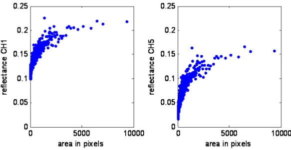
The reflectance distribution (Eq. 4) is a product of two functions with opposing trends. The total area per cloud size is larger for the small clouds (A(a)=b/am−1) while the av-erage reflectance is greater for larger (thicker) clouds. However, both the data and 10

the analytical derivation (which can be found Appendix B) show that for our measured slopes of the power-law distribution, the total-area-function decreases faster than the total-reflectance-function increases as a function of the cloud size. Therefore the re-flectance contribution from the small clouds is greater than that of the larger ones (Fig. 1, lower panels). For all 5 scenes, most of the contribution to the total reflectance 15

originates from the smaller clouds. Specifically, from 15% to 50% (mean of 31% with standard deviation of 14%) comes from clouds with area below 1 km2.

The steep size distribution implies that the smaller clouds dominate the contribu-tions to cloud number, total cloud area and reflected radiation. It is therefore expected that sensor resolutions much coarser than most clouds sizes of this type affect these 20

properties of the cloud field as inferred from space. Indeed, upon reducing the resolu-tion, the slopes of the distributions of all five fields become smaller (in absolute value) from an average of 1.3±0.1 to 1.1±0.1 showing shifting of the distribution toward the larger clouds (Fig. 2). These changes are due to averaging out the smaller clouds that are distant enough from other clouds and for which the average reflectance of 25

the cloud and the surrounding background does not pass the threshold, while on the other hand, enlarging further the larger clouds by incorporating small holes and nearby clouds (Fig. 3).

(9)

ACPD

8, 6379–6407, 2008

Interactive Discussion These changes in the size distribution of clouds drive changes in all other

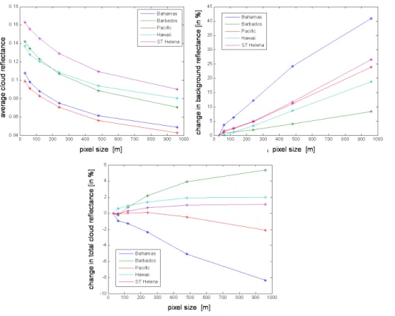
proper-ties of the cloud field. The proportion of apparently cloudy to apparently cloud- free changes, as well as the optical properties of the clouds and background. The over-all cloud fraction increases as large clouds become larger at a rate faster than that at which small clouds disappear into the apparent cloud-free zone. For all 5 fields 5

the cloud fraction at MODIS resolution (mean 30%, standard deviation (STD) 11%) is double that of the original Landsat resolution (mean 15%, STD 6%) (Table 1). The increased cloud fraction decreases the cloud-average reflectance to less than half, as more background pixels are classified as cloud. The background reflectance increases to an average of more than 23%, as more isolated small clouds are “dissolved” into 10

the “twilight zone” while the cloud reflectance distribution is shifted dramatically toward the larger clouds. Eventually, the reflectance appears to be mostly due to a few large clouds and assumes a completely different spatial distribution (Fig. 4).

How is the total energy redistributed in the coarse resolution? Even though the total reflectance (used as a direct measure of the solar energy reflected back to space) is 15

preserved when reducing the resolution, the pattern of contributions from clouds and cloud-free atmosphere is changed dramatically. The end-result depends on the inter-play between the increase in total cloud area and the decrease in cloud-average re-flectance. Figure 4 (bottom-left) shows that for scenes with low initial cloud reflectance the total cloud reflectance decreases with decreasing resolution while for others it in-20

creases.

What is the apparent direct aerosol forcing due to the contribution of the small clouds misclassified as background? The aerosol forcing, defined as any deviation from the natural balance, is calculated by comparing the real top-of-the-atmosphere fluxes from the theoretical fluxes with (clean) background aerosol (Kaufman et al., 2001). There-25

fore for clean areas, the increase in background reflectance will be translated to a positive increase in the local aerosol loading. The mean change in the background reflectance between 30 m and 960 m is 0.0019±0.0006. Since clouds have a relatively flat spectral dependence in solar wavelengths (shown for one case in Appendix C),

(10)

ACPD

8, 6379–6407, 2008

Interactive Discussion this reflectance change corresponds to an apparent aerosol optical depth (AOD) of

approximately 0.02 to 0.03 consisting of mostly coarse mode aerosol (Remer et al., 2005). This additional “artificial” AOD will be interpreted as an average 24 h forcing of −0.8±0.2 W/m2, or about 15% to 20% of the total global aerosol effect estimated from MODIS aerosol retrievals (Remer and Kaufman, 2006). While this may not seem to be 5

a large forcing if only local, the spatial coverage of scattered cumulus cloud fields is large. Shallow cumulus cloud fields cover more than 10% of all oceans and more than 16% of the area between 40◦N to 40◦S (Warren and Hahn, 2007).

4 Summary and conclusions

We have shown that in a sparse cumulus cloud field, small clouds are extremely im-10

portant. The smallest detectable clouds contribute the most to the total cloud area and the mean field reflectance (Appendix B). The portion of small clouds that are “stand-alone”, and far enough from other clouds, have the highest likelihood of being dissolved into the so-called twilight zone and to be labeled as “cloud-free” in coarser resolution imagery (Fig. 3).

15

We show that cloud sizes obey a power-law distribution with a slope bounded be-tween 1 and 2 (1<m<2). This finding, along with a reflection distribution and scale

effect analysis imply that:

1. The distribution of the total area with respect to cloud size will also be a power law with slope (_{m−1) 0<m−1<1 and therefore decreases monotonically as the} 20

cloud area increases (see Appendix A).

2. The reflectance per cloud size increases slower than the rate at which the cloud area per cloud size decreases. Therefore, small clouds contribute significantly to the total cloud reflectance (an analytical analysis and discussion are given in 25

(11)

ACPD

8, 6379–6407, 2008

Interactive Discussion Appendix B).

3. The slopes of the distributions decrease with decreasing spatial resolution implying that an increasing amount of reflectance is falsely attributed to larger clouds.

5

4. The apparent direct aerosol forcing (surface cooling) due to classifying cloud pix-els as cloud-free in the sparse cumulus fields is on the order of −0.8±0.2 Wm−2

for the cloud field area. 10

5. The Landsat resolution of 30 m was the highest resolution used in this analysis. The nature of the power-law distribution of cloud areas suggests that for any resolution, significant cloudy parts will be missed. Since there is no physical limit at the 30 m resolution this distribution possibly extrapolates toward finer resolutions. This suggests that small clouds of only a few meters may contribute 15

significantly to the total cloud fraction and reflectance.

Appendix A

More on the power-law distribution of clouds

20

In the paper we show that the size distribution of shallow marine cumulus clouds follows a power-law of the form:

(12)

ACPD

8, 6379–6407, 2008

Interactive Discussion wheren(a) is the number of clouds per given area a (expressed in pixels for simplicity),

b is a constant equal to the number of clouds with an area of one pixel and m is

the power exponent of the distribution. From the above, the distribution of areasA(a)

covered by clouds with areaa is given by a power law, but with an exponent m−1: A(a) = an = b

am−1 (A2)

5

In the paper we show that m is bounded between 1 and 2 (1<m<2). From these

basic facts alone, one can infer essential information on the properties of the distribu-tion of areasA(a) and the moments of the distribution. Because the exponent of the

area power-law is larger than zero (0<m−1<1), the area A(a) distribution will decay

as clouds become larger which implies that small clouds contribute more to the total 10

cloud area. Moreover, a cloud number distribution withm>1 (Eq. A1) implies that the

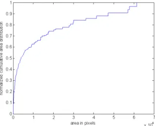
number of clouds goes down rapidly (faster than 1/a) as their size increases. Figure A1 shows that 30% of the total cloud area comes from the first 1000 pixels (area of less than 1 km2) for the Ascension Island scene.

In the paper it is shown that the reflectance distribution is a product of two functions 15

with opposing trends. The total area per cloud size is greater for the smaller clouds, while the average reflectance is greater for the larger (thicker) clouds (Fig. A2).

We define the unitless cloud-integrated reflectance R as the reflectance from all

clouds given by:

R =X i Ri = X i riniai (A3) 20

Summing reflectances of different clouds is permitted in our case because we deal with a relatively small area with uniform observational and solar geometry. The total reflectance so defined is thus used here as a direct measure of the total energy re-flected back to space. When calculating the distribution of the total reflectance as a function of the cloud size, the contribution of the small cloud to the total reflectance is 25

(13)

ACPD

8, 6379–6407, 2008

Interactive Discussion the reflectance as a function of cloud size. Figure A3 shows the reflectance

distribu-tion as a funcdistribu-tion of the cloud area. It is clearly shown that the area takes over the reflectance trend. Therefore the reflectance of the smallest clouds contributes more to the total cloud reflectance.

Appendix B

5

Analytical analysis of the reflectance distribution function

Assuming that the optical thickness τ of a cloud is, among others, a function of its

geometrical thicknessh. If the cloud maintains an aspect ratio that is proportional to

the cloud’s area we can write the following: 10

τ ∝ hβ h ∝ a1/2

For the general case if the aspect ratio does not change fast as a function of the cloud area, we can approximate the cloud optical thickness using the area with two free parameters (c1,α):

τ = c1aα (B1)

15

It can be shown that for the range of optical thicknesses between 0 and 20, appropriate for our shallow cumulus cloud fields the nadir reflectance calculated with the multiple scattering code (DISORT) can be fit with a simple expression of the form:

r = Bτ

2 + Bτ (B2)

whereB assumes values approximately between 0.1 and 0.2 depending on the SZA

20

(14)

ACPD

8, 6379–6407, 2008

Interactive Discussion drop size distribution. This analytical expression is similar to the one for albedo in the

two-stream approximation in the case of conservative scattering (Bohren 1980). Hence, the total reflectance per cloud area can be written as:

R(a) = rna = Ga

α

2 + Gaαba

(1−m) _(B3)

where G=Bc1 is therefore a collective parameter that includes all dependencies on

5

solar zenith angle, cloud optical properties such as single-scattering albedo and asym-metry factor, and the proportionality parameterc1between the cloud area andτ.

The conditions under whichR(a) becomes maximum can be explored by zeroing its

first derivative with respect to cloud area.

d R d a = Gb 2 + Gaα(1 + α − m)a (_α−m) − Gb (2 + Gaα₎2a (1+α−m)_Gαa(_α−1) (B4) 10

For the derivative d R_{d a} to become zero the following condition should be met:

m − 1 = 2α

2 + Gaα (B5)

The left hand side of the equation depends on the slopem of the size (area) distribution

and the right hand side depends on parameters related to the geometrical and optical properties of the clouds (G and α).

15

The analytical reflectance functionR(a) will rich its maximum value when the area a

will satisfy Eq. (B5). Note that the right hand part of Eq. (B5) becomes maximum when the cloud area approaches zero and at this point depends only onα, the exponent that

translates area toτ.

m − 1 = α (B6)

20

Therefore, ifα<m−1, R(a) will not have a maximum and will go monotonically down

suggesting that the highest contribution to the reflectance comes from the smallest clouds (of 1 pixel).

(15)

ACPD

8, 6379–6407, 2008

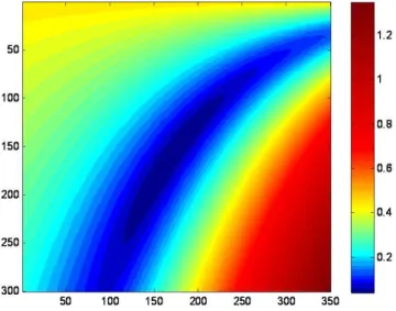
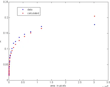
Interactive Discussion Next, we estimate the empirical parametersG and α from the data by varying their

values and comparing the theoretical reflectance calculations from Eq. (B2) to the ac-tual (measured) reflectance as a function of the cloud area and seeking the values that minimize the error (inL2). Figure B1 shows a clear, well define minimum suggesting that the agreement between theory and measurements occurs for an unambiguous 5

point inG−α space. Figure B2 shows the reflectance comparison for the optimal of G

andα values (those providing minimum reflectance error in G−α space).

For the Polynesian Landsat scene _{G=0.0322 and α=0.2690 for band 5, and}

G=0.173 and α=0.125 for band 1. Inserting the above values of α into Eq. (B6) shows

that any slopem>1.269 for band 5 and m>1.125 for band 1 will result in the smallest

10

area clouds to contribute the most to the integrated reflectance. Indeed, this is clearly shown in the data (Fig. A3).

This method of retrievingα and G, statistically form the data can be a powerful tool

for structural and microphysical analysis of small clouds. Together with the use of two wavelengths (absorbing and non-absorbing, Nakajima and King, 1990) to retrieve the 15

cloud optical thickness and the droplets effective radius per cloud, we retrieve α and

G statistically for the whole field, and link them to the cloud optical properties and

geometry. While the retrieval of cloud optical thickness and droplets effective radius of a small single cloud suffers form the 3-D effect (e.g. the plain parallel assumption can not hold for small clouds, Wen et al., 2007) and small S/N ratio, here we retrieve 20

statistical parameters for the whole cloud field. We can do so for many wavelengths, absorbing and non-absorbing, using any reflectance and the size distribution, to gain extra information such as an estimation for the clouds 3-D effect as a function of the cloud size and the clouds aspect ratio.

(16)

ACPD

8, 6379–6407, 2008

Appendix C

Forcing analysis for the Landsat’s blue and red wavelengths

We performed the analysis in the NIR (1600 nm) to minimize the contribution of molecular scattering, aerosols and cloud 3-D effects (Wen et al., 2007). Also, the 5

Landsat NIR channel (ch-5) is known to be superior with respect to signal-to-noise (http://imaging.geocomm.com/features/sensor/landsat7). We nevertheless repeated the analysis for the Landsat blue (480 nm) and red (660 nm) channels of the Bahamas scene. The results are shown in Table C1. Since clouds have an almost flat spectral dependence in the visible to NIR range the differences in total reflectance are similar. 10

As discussed above, the reflectance distribution combines the contributions of two functions with opposing tendencies. The total cloud area per cloud size goes down fast (as a power-law function) for the large clouds while the reflectance goes up. The following figure (Fig. C1) shows the cumulative reflectance as a function of the cloud size for all 3 wavelengths.

15

Acknowledgements. This paper is dedicated to the memory of Y. J. Kaufman, a dear friend and

a brilliant scientist. This research was supported in part by the Israel Science Foundation (grant 1355/06) and NASA’s Radiation Sciences Program and Interdisciplinary Studies. We thank the reviewer for helpful comments. I. Koren is incumbent of the B. H. Swig and J. D. Weiler career development chair. The source for this dataset was the Global Land Cover Facility, 20

http://www.landcover.org.

References

Cahalan, R. F. and Joseph J. H.: Fractal Statistics of Cloud Fields, Mon. Weather Rev., 117, 261–272, 1989.

Feingold, G., Jiang, H. and Harrington, J. Y.: On smoke suppression of clouds in Amazonia, 25

(17)

ACPD

8, 6379–6407, 2008

Interactive Discussion Kaufman, Y. J., Smirnov, A., Holben, B. and Dubovik, O.: Baseline maritime aerosol

methodol-ogy to derive the optical thickness and scattering properties, Geophys Res. Lett., 28, 3251– 3254, 2001.

Koren, I. and Joseph, J. H.: The histogram of the brightness distribution of clouds in high resolution remotely sensed images, J. Geophys. Res., 105(D24), 29 369–29 377, 2000. 5

Koren I., Kaufman, Y. J., Remer, L. A., and Martins, J. V.: Measurement of the Effect of Amazon Smoke on Inhibition of Cloud Formation, Science, 303, 1342–1345, 2004.

Koren, I., Remer, L. A., Kaufman, Y. J., Rudich, Y., and Martins, J. V.: On the twilight zone be-tween clouds and aerosols, Geophys. Res. Lett., 34, L08805, doi:10.1029/2007GL029253, 2007.

10

Krijger, J. M., van Weele, M., Aben, I., and Frey, R.: Technical Note: The effect of sensor resolution on the number of cloud-free observations from space, Atmos. Chem. Phys., 7, 2881–2891, 2007,

http://www.atmos-chem-phys.net/7/2881/2007/.

Nakajima, T. and King M. D.: Determination of the optical thickness and effective particle radius 15

of clouds from reflected solar radiation measurements. Part I: Theory, J. Atmos. Sci., 47, 1878–1893, 1990.

Neggers, R. A. J., Jonker, H. J. J., and Siebesma, A. P.: Size statistics of cumulus cloud populations in large-eddy simulations, J. Atmos. Sci., 60, 1060–1074, 2003.

Newman, M. E. J.: Power laws, Pareto distributions and Zipf’s law, Contemp. Phys., 46(5), 20

323–351, 2005.

Plank, V. G.: The Size Distribution of Cumulus Clouds in Representative Florida Populations, J. Appl. Meteorol., 8, 46–67, 1969.

Remer, L. A., Kaufman, Y. J., Tanre, D., Mattoo, S., Chu, D. A., Martins, J. V., Li, R. R., Ichoku, C., Levy, R. C., Kleidman, R. G., Eck, T. F., Vermote, E., and Holben, B. N.: The MODIS 25

aerosol algorithm, products and validation, J. Atmos. Sci., 62, 947–973, 2005.

Remer, L. A. and Kaufman Y. J.: Aerosol direct radiative effect at the top of the atmosphere over cloud free ocean derived from four years of MODIS data, Atmos. Chem. Phys. , 6, 237–253, 2006.

Rodts, S. M. A, Duynkerke, P. G., and Jonker, H. J. J.: Size distributions and dynamical prop-30

erties of shallow cumulus clouds from aircraft observations and satellite data, J Atmos. Sci., 60(16), 1895–1912, 2003.

(18)

ACPD

8, 6379–6407, 2008

http://www.atmos.washington.edu/CloudMap/, 2007.

Tanre, D., Kaufman, Y. J., Herman, M., and Mattoo, S.: Remote sensing of aerosol proper-ties over oceans using the MODIS/EOS spectral radiances, J. Geophys. Res.-Atmos., 102, 16 971–16 988, 1997.

Wielicki, B. A. and Welch, R. M.: Cumulus Cloud Properties Derived Using Landsat Satellite 5

Data, J. Appl. Meteorol., 25, 261–276, 1986.

Wen, G., Marshak, A., Cahalan, R. F., Remer, L. A., and Kleidman, R. G.: 3-D aerosol-cloud radiative interaction observed in collocated MODIS and ASTER images of cumulus cloud fields, J. Geophys. Res., 112, D13204, doi:10.1029/2006JD008267, 2007.

Xue, H. and Feingold, G.: Large-Eddy Simulations of Trade Wind Cumuli: Investigation of 10

Aerosol Indirect Effects, J. Atmos. Sci., 63(6), 1605–1622, 2006.

Zhao, G. and Di Girolamo, L.: Cloud fraction errors for trade wind cumuli from EOS-Terra instruments, Geophys. Res. Lett., 33, L20802, doi:10.1029/2006GL027088, 2006.

Zhao, G. and Di Girolamo, L.: Statistics on the macrophysical properties of trade wind cumuli over the tropical western Atlantic, J. Geophys. Res., 112, D10204, 15

(19)

ACPD

8, 6379–6407, 2008

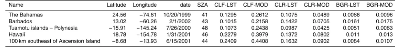
Table 1. Information on the five Landsat scenes analyzed in this study.

Name Latitude Longitude date SZA CLF-LST CLF-MOD CLR-LST CLR-MOD BGR-LST BGR-MOD The Bahamas 24.56 −74.61 10/20/1999 41 0.1295 0.2612 0.1075 0.0489 0.0068 0.0096 Barbados 13.02 −60.26 2/1/2002 43 0.1015 0.2158 0.1422 0.0705 0.0161 0.0175 Tuamotu islands – Polynesia −15.91 −145.24 7/26/2000 48 0.1073 0.2438 0.0987 0.0425 0.0051 0.0063 Hawaii 18.78 −154.78 1/31/2001 46 0.2279 0.3979 0.1372 0.0802 0.011 0.013 100 km southeast of Ascension Island −8.68 −13.93 6/15/2001 44 0.2409 0.4408 0.1632 0.0902 0.0084 0.0107

SZA Solar Zenith angle.

CLF-LST Cloud fraction in the fine (30 m) resolution. CLF-MOD Cloud fraction in the coarse (960 m) resolution.

CLR-LST Cloud average reflectance in the fine (30 m) resolution. CLR-MOD Cloud average reflectance in the coarse (960 m) resolution. BGR-LST Cloud-free average reflectance in the fine (30 m) resolution. BGR-MOD Cloud-free average reflectance in the coarse (960 m) resolution.

(20)

ACPD

8, 6379–6407, 2008

Table C1. The resolution effect in the blue, red and NIR Landsat channels.

Wavelength Background reflectancea Mean cloud reflectanceb

(nm) difference difference

480 0.0026 0.0532

660 0.0028 0.0597

1600 0.0028 0.0587

a

differences in background reflectance between 960 m and 30 m resolution.

b

(21)

ACPD

8, 6379–6407, 2008

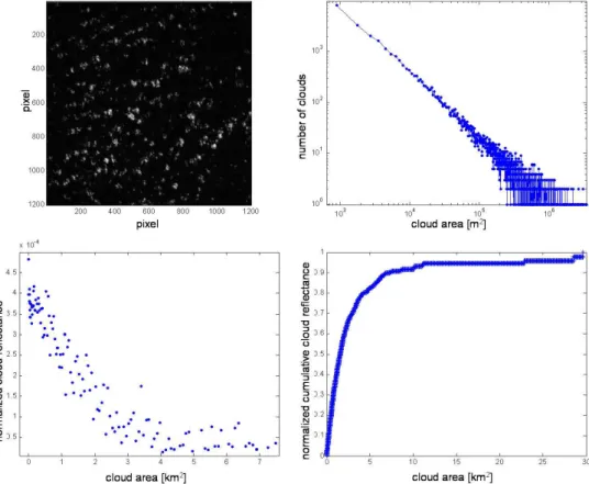
Fig. 1. Sparse cloud field over the Pacific Ocean near Tahiti. Top-left: Magnified portion of the

cloud field with pixel resolution of 30 m. Top-right: size distribution of the clouds. Note the large spread of the results for the large cloud sizes due to small number of samples in these bins. Bottom-left: normalized (unit integral) total per cloud area reflectance as a function of the cloud size. Bottom-right: cumulative cloud reflectance showing that most of the reflectance comes from the smaller clouds.

(22)

ACPD

8, 6379–6407, 2008

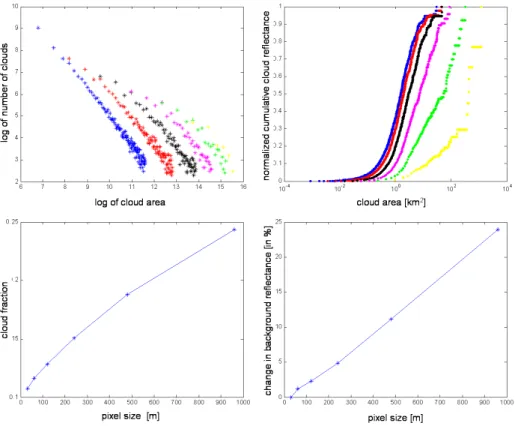
Fig. 2. The effect of resolution on the size distributions of a sparse cloud field over the Pacific

Ocean near Tahiti. Top-left: log-log cloud size distributions for resolutions ranging from the original 30 m Landsat resolution (blue) to approximate 1 km MODIS resolution (yellow). Top-right: cumulative distribution of the cloud reflectance (normalized to unity) for all resolutions. Note how the size distribution (left) and the energy distribution (right) are shifted toward larger clouds as the resolution decreases. Bottom-left: change in cloud fraction from 12% in the highest to 24% in the coarsest resolution. Bottom-right: the effect of resolution on the ”non-cloudy” pixels, showing a 24% increase in reflectance.

(23)

ACPD

8, 6379–6407, 2008

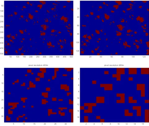
Fig. 3. Cloud mask for a sparse cumulus cloud field as inferred by using the same threshold

at 4 different spatial resolutions. The upper-left panel is for the original Landsat resolution and the lower-right panel is for a MODIS-equivalent resolution. Note how the small clouds far from other clouds are “dissolved” into the background while small clouds, holes between clouds, and background pixels next to large cloud edges are all classified as clouds. The cloud fraction of the finer Landsat resolution is 11% and of the coarser MODIS resolution is 24%. The mean cloud reflectance at the Landsat resolution is more than twice that at MODIS resolution which has 23% higher background reflectance.

(24)

ACPD

8, 6379–6407, 2008

Fig. 4. The effect of resolution on all 5 sparse cloud fields. Top-left: average cloud reflectance.

Top-right: changes in the background reflectance. Bottom: changes in total cloud energy (reflectance).

(25)

ACPD

8, 6379–6407, 2008

Fig. A1. Cumulative-distribution function of the total cloud area for the Ascension Island scene.

(26)

ACPD

8, 6379–6407, 2008

Fig. A2. Cloud reflectance as a function of the cloud area. The reflectance is defined here as

the directional (nadir) radiance normalized by the downwelling solar irradiance in the particular band. The left panel is for the Landsat blue channel (0.47µm), and the right panel is for Landsat

(27)

ACPD

8, 6379–6407, 2008

Fig. A3. Normalized total cloud reflectance as a function of cloud area for the Landsat blue

channel (0.47µm, blue dots), and for Landsat Band 5 (1.63 µm, red dots) after logarithmic

binning to correct for small number fluctuations in the large cloud bins. Note that the reflectance of the smallest clouds is normalized to unity and in both cases contributes much more to the total cloud reflectance than the next available cloud size.

(28)

ACPD

8, 6379–6407, 2008

Fig. B1. Nadir reflectance error inG−α space for Band 5 of the Polynesian Landsat scene. The

vertical axis shows convertedG values (G=0.0002*y) while the horizontal axis shows converted α values (α=0.1+0.001x).

(29)

ACPD

8, 6379–6407, 2008

Fig. B2. Reflectance comparison for the optimal ofG and α value (those providing minimum

(30)

ACPD

8, 6379–6407, 2008

Fig. C1. Cumulative reflectance distribution as a function of cloud size for the Bahamas scene.