Development of an econometric model for dynamic management of recession risk in equity portfolios : construction of an empirical measure of time-varying recession risk : estimation of cross-sectional differences in recession risk exposure among equities a

Development of an econometric model for dynamic management of recession risk in

equity portfolios. Construction of an empirical measure of time-varying recession risk.

Estimation of cross-sectional differences in recession risk exposure among equities and

associated differences in risk premia.

MASSACHUSETTS INSTITUTE OF TECHNOLOGY

By

Kyriakos Chousakos

JUN 152011

BSc. in Finance and Accounting

LIBRARIES

Athens University of Economics and Business, 2010

_ARCHVES

SUBMITTED TO THE MIT SLOAN SCHOOL OF MANAGEMENT IN PARTIAL FUFILLMENT OF THE REQUIREMENTS FOR THE

DEGREE OF MASTER OF FINANCE

AT THE

MASSACHUSETTS INSTITUTE OF TECHNOLOGY JUNE 2011

© 2011 Kyriakos Chousakos. All Rights Reserved. The author hereby grants to MIT permission to reproduce and to distribute publicly paper and electronic copies of this thesis document in

whole or in part in any medium now known or hereafter created.

Signature of Author:

MIT Sloan School of Management

May 6, 2011

Certified By:

Leonid Kojgn Nippon Telephone and Telegraph Professor of Finance

Thesis Supervisor

Accepted By:

Leonid Kbgan Nippon Telephone and Telegraph Professor of Finance Program Director, Master of Finance MIT Sloan School of Management

Development of an econometric model for dynamic management of recession risk in

equity portfolios. Construction of an empirical measure of time-varying recession risk.

Estimation of cross-sectional differences in recession risk exposure among equities and

associated differences in risk premia

By

Kyriakos Chousakos

Submitted to the MIT Sloan School of Management on May 6, 2011 in partial fulfillment of the requirements for the degree of Master of

Finance

ABSTRACT

Recessions are an inherent part of economic cycles. During the last decade we have experienced two extended periods of significant economic slowdown accompanied by major downturns in most of the asset classes and especially in equities. Investors during recessions suffer from severe losses and diversification does not provide the optimal solution. Through the development of an econometric model for dynamic management of recession risk in equity portfolios based on an empirical measure of time-varying recession risk, I plan to estimate cross-sectional differences in recession risk exposure among equities and associated differences in risk premia. The analysis is expanded on an industry level, where among industries clear patterns are identified in terms recession risk exposure. In the last part of the report

I explore the possibility of creating a trading strategy which is able to generate significant performance

benefiting from the market underreaction to recession risk. Thesis Supervisor: Leonid Kogan

Acknowledgements

I am grateful to Professor Leonid Kogan for his generous mentorship and for his insightful guidance

Table of Contents

INTRODUCTION ... 3 LOGIT M ODEL...5 General approach... 5 Factor specification...5 Term spread... 5 Credit Spread...6

The S&P 500 returns...6

Sample Construction...6

Estimation Results, Discussion ... 7

ESTIM ATION OF THE LOADINGS...10

General approach...10

Sample Construction... 11

M ethodology ... 11

Vasicek Betas ... ₁₁

RECESSION FACTOR AS RISK FACTOR ... 12

General approach...12

Sample Construction... 13

M ethodology ... 13

Estimation Results, Discussion ... 14

INDUSTRY ANALYSIS... 14

General approach...14

Data Specification...15

M ethodology ... 15

Results and Discussion ... 16

ROBUSTNESS ANALYSIS. IM PLICATIONS... 20

General approach...20

Data Specification... 21

M ethodology ... 21

Discussion, Results ... 22 1

Properties of the created portfolios ... 22

Beta stability... 23

Consistency of the procedure ... 23

Recession portfolio performance ... 24

CONCLUSION ... 30

REFERENCES... 31

Table of Figures

Figure 1. Scatter plot of fitted probabilities over the first half and the entire sample of explanatory variables...9

Figure 2. Comparison of predicted probabilities of recession with the NBER recession periods on a weekly basis...9

Figure 3. Industry normalized concentration per decile ... 16

Figure 4. Shape of the first principal component applied on the industry normalized contribution at each decile ... 17

Figure 5. Regression results of the intertermporal normalized industry concentration over the number of deciles ranging from 1 to 10, industry coefficients ... 19

Figure 6. Comparison of porfolio profit-loss with NBER periods of recession... 25

Figure 7. Joint plot of the first lag of the residuals level and profit-loss from the proportional exposure to full scale portfolio ... 25

Figure 8. Comparison of alternative portfolio levels with NBER periods of recession ... 26

Figure 9. Joint plot of lagged residuals and profit-loss of the long position component of the full scale portfolio... 27

Figure 10. Joint plot of lagged residuals and profit-loss of the short position component of the full scale portfolio... 27

Figure 11. Joint plot of lagged residuals and profit-loss of the residual weighted exposure to within industry portfolio... 28

Figure 12. Joint plot of lagged residuals and profit-loss of the long position component of the within industry portfolio... 29

Figure 13. Joint plot of lagged residuals and profit-loss of the short position component of the within industry portfolio...29

INTRODUCTION

Recessions are an inherent part of economic cycles. During the last ten years we have experienced two extended periods of significant economic slowdown which were accompanied by major downturns in most of the asset classes and particularly in equities. Investors during recessions suffer from severe losses and simple diversification among equities does not seem to be the optimal solution which can provide a 'safety net' to an equity portfolio. In this report I will attempt to construct an econometric model for dynamic management of recession risk in equity portfolios.

A first step towards this is the construction of an empirical measure of time-varying recession risk. This

can be implemented by a binary LOGIT model estimated using macroeconomic factors such as term spreads, credit spreads, and the S&P 500 returns as explanatory variables. This model attempts first, using quarterly data, to explain, and then with the use of weekly data, to predict the probability by which a recession will occur in the next quarter. The model is tested for overfitting and the predicted probabilities are plotted against the main periods of recession as they are identified by the National Bureau of Economic Research (NBER).

The loadings (betas) of publicly traded stock equities on the recession risk factor are estimated based on the percentage changes in the probability of recession generated by the LOGIT model. These stocks constituted the US equity market from 1962Q1 to 2010Q3. During the time span of the analysis, 45 rolling five-year betas are calculated leading to a same number of annual groups of beta estimations. The loadings are adjusted using the Vasicek technique which minimizes the loss due to misestimation, and takes into account knowledge of the prior distribution of the parameters.

The Fama - MacBeth procedure is applied on the Vasicek adjusted cross-sectional betas to obtain an indication of whether the recession factor is actually a risk factor for exposure to which investors demand a risk premium. After regressing the cross-sectional Vasicek adjusted betas over the excess returns of the stocks for each one of the 44 years for which data were available, and accounting for the standard errors, the change in the probability of recession is identified as a risk factor for exposure to which investors

demand a risk premium as compensation.

Also, the analysis is expanded on an industry level, where I attempt to identify patterns in several industries with respect to their exposure to recession risk. Based on Kenneth French's industry classification of the SIC codes, each stock is assigned to a particular industry. The stocks are sorted according to their Vasicek adjusted beta loadings and they are arranged into deciles. For every industry I

calculate its concentration in each one of the deciles and using principal component analysis it becomes obvious that particular industries show specific patterns. In order to identify the direction of the patterns the industry normalized concentrations are regressed over the number of deciles and from this analysis it becomes clear that food products, household consumer goods, utilities, and telecommunications seem to have countercyclical behavior, while clothing, textiles, and aircraft, ships and railroad equipment show cyclical behavior.

Finally, two portfolios consisting of long positions on stocks with high loadings on the risk factor, and short positions on stocks with low loadings on the risk factor are constructed. The first portfolio contains long positions on the last decile and short positions on the first, while the second is formed on long and short positions on the last and the first decile within each industry. The excess returns of both portfolios are regressed over the factors of the Fama - French three factor model. From this analysis it becomes obvious that a part of the variability in the returns of the first portfolio is explained by the SMB and HML factors. Also, the loadings on these two factors are negative indicating that big companies with low book to market ratio are better hedges during recessions. On the other hand for the second portfolio a safe conclusion regarding its exposure to the three risk factors could not be drawn, but both portfolios seem to generate negative alpha. Also, the Vasicek betas are tested for their intertemporal stability and the performance of the first portfolio is calculated during periods of recession. Last, the first portfolio returns are regressed over the lagged residuals of the change in the risk factor proving that the market underreacts to changes in the risk factor indicating that that it is feasible to create a trading strategy which could benefit from this underreaction.

This report is organized as follows: In the beginning I describe the LOGIT model I estimate in order to predict the probability of recession in the next quarter. There is a short explanation of the factors used in the estimation, of the estimation results and the results from the robustness check of the model, while the generated probabilities are plotted against recession periods as they are specified by the National Bureau of Economic Research. In the next section I attempt a description of the calculation of the loadings (betas) on the recession factor, where I refer to the data used in this analysis and the Vasicek calculations performed for the adjustment of the estimated loadings. Following, there is a description of the Fama -MacBeth methodology employed in this context for the specification of the recession factor as a risk factor. In the subsequent industry analysis I attempt to identify patterns among industries and particular industries are identified as potential hedges against recession. In the last part of the report. I create two portfolios with long and short positions based on the exposure of the stocks on the recession factor and the industry they belong to. Their performance is compared to changes in the risk factor and regressed over the factors of the Fama - French model. In the same part, I check for the stability of the calculated

betas, the performance of the constructed portfolios during recessions, and whether an investor can benefit from market underreaction to recession risk. Finally, the conclusion sumnarizes the basic findings and makes a number of reconnendations in terms of future work.

LOGIT MODEL

General approach

The first step towards the estimation of an econometric model for dynamic management of recession risk in equity portfolios is the construction of an empirical measure of time-varying recession risk. This can be described by a binary LOGIT model which using macro-economic factors such as term spreads, credit spreads, and the S&P 500 returns attempts first to explain and then to predict the probability by which a recession will occur in the next quarter. The model is expressed as follows:

1 Pt = 1+e-Pt

Where: xt is a vector of the constant term, term spreads, credit spreads, and the S&P 500 returns; fl is a vector of factor sensitivities; pt is the probability that recession will occur in the next quarter; t is the month the levels of term spreads, credit spreads, and the S&P 500 returns are observed.

Factor specification

Term spread

The slope of the Treasury yield is a leading economic indicator, whose inversion has been an indication of

recession. Historically the term spread defined as the ten-year Treasury Bond rate less the three-month

Treasury Bill has exhibited a positive statistical relationship with real GDP growth over subsequent

quarters, and a negative statistical relationship with the probability of recession. The rationale behind the

use of term spreads as an indicator in the model derives from the expectations hypothesis which neglects

liquidity preference premiums and states that the forward rate equals the market consensus expectation of

the future short interest rate. The term spread is a measure of the standpoint of the monetary policy. The

lower the term spread, the more restrictive the monetary policy indicating an imminent recession. It is

clear that under the expectations hypothesis the term spread does not capture all the information in the

yield curve regarding the probability of a recession. However, it can be a valuable indicator of the

economic climate and the monetary policy. In the existing literature there have been several papers

studying the predictive power of the yield curve for growth indicating that this predictive power has weakened since the 1980s, but they have not been able to prove a structural break in the relationship between the term spread and the occurrence of recessions.

Credit Spread

The credit spread or otherwise the yield spread is defined as the difference in yield between different bonds due to different credit quality. It reflects the additional net yield an investor can earn from a bond with more credit risk relative to one with less. For the purposes of this analysis this factor is defined as the yield of a Moody's Baa rated bond less the yield of a Moody's Aaa rated bond, both with a duration of twenty years. Research has shown that the credit spread behaves counter-cyclically as it narrows during business cycle expansions and widens during contractions. This finding holds not only for the postwar period, but also for the period from 1925 to the present. There has also been evidence that the credit spread leads the business cycle. Finally, it has been documented that turning points of the credit spread contain significant information about future turning points of the business cycle. It is clear that the credit spread can be a leading indicator of macroeconomic business conditions and turning points on its curve can predict business cycle turning points.

The S&P 500 returns

The use of the S&P 500 returns into the model is based on the observation that the market is alert of

possible changes in the economic cycles and incorporates these changes into the company valuations

expressed by company capitalization. As a result of this observation a negative relationship between the

market returns and the probability of recession is expected. The intuition behind this relationship states

that when investors realize that a recession is imminent, they demand a higher risk premium to

compensate for the lower returns they will receive during the recession period. It is also generally true

that company profitability will be lower during this period and this fact has to be incorporated into the

company valuations, driving prices lower.

Sample Construction

For the estimation of the model, data regarding the macroeconomic factors (independent variables) are

downloaded from the St. Louis Federal Reserve database. More specifically, for the calculation of the

term spreads I use the ten-year Treasury Constant Maturity rate minus the three-month Treasury Bill rate

on a quarterly basis from 1962Q1 to 2010Q3. The credit spreads are calculated based on the difference

between the Moody's Seasoned Baa Corporate Bond Yield and the Moody's Seasoned Aaa Corporate

Bond Yield on a quarterly basis from 1962Q1 to 2010Q3. For the calculation of the yields Moody's tries to include bonds with remaining maturities as close as possible to 30 years and drops bonds with a remaining life below 20 years, bonds susceptible to redemption, and bonds with change in the credit rating. The S&P returns are calculated on the quarterly levels of the S&P 500 stock index for the time period of the analysis. The S&P 500 index includes 500 leading companies in leading industries of the

U.S. economy which are publicly held on either the NYSE or NASDAQ, and covers 75% of the U.S.

stock capitalization.

The dependent variable indicates the occurrence of recession. I decided to diverge from the tight definition of recession given by the NBER and for the purposes of this analysis recession is defined as every decline of the real GDP level. As a result, data regarding Real Domestic Product are downloaded from the U.S. Department of Commerce: Bureau of Economic Analysis on a quarterly basis from 1962Q1 to 2010Q3. The periods of recession were identified by a dummy variable which takes the values one in the occurrence of recessions and zero during periods of economic growth.

For the prediction using the model within the time span of the analysis, data for the same macroeconomic factors are downloaded from the St. Louis Federal Reserve on a weekly basis for the time span of the analysis.

Estimation Results, Discussion

Turning to results of the model estimation, the coefficient on the ten-year over three-month term spread is negative and statistically significant', verifying the underlying historical statistical relationship between this factor and the economic cycle. The coefficient on the credit spread is positive and statistically significant, reaffirming the intuition behind the relationship between credit spreads and recession occurrence. Finally, the coefficient on the S&P returns is negative and statistically significant, confirming the rationale behind the use of this factor as an explanatory variable. The LOGIT regression results are

summarized at table 1.

Table 1. LOGIT regression results

Coeeffiients T-stats P-values

Constant Factor -3.7434 -5.5215 0.0000

Term Spreads -0.5320 -2.5106 0.0121

Credit Spreads 2.1722 3.7353 0.0002

S&P 500 Returns -19.0442 42957 0.0000

The negative coefficient of the term spread as stated above verifies the underlying historical statistical

relationship between this factor and the likelihood of recession. This indicates that a decrease in the

spread is likely to signal an increased probability of recession. The positive coefficient of the credit

spread is not a surprising finding as it is naturally expected to narrow during business cycle expansions

and to widen during contractions. Finally, the negative sign of the S&P 500 returns is in line with the

rationale analyzed in the factor specification part, where negative returns are considered an indication of

an imminent recession.

A common issue that occurs in the estimation of a statistical model is overfitting. This happens when a

statistical model describes random error or noise instead of the underlying relationship of the variables. It

is common in complex models and provides an indication of poor predictive performance of the estimated

model. A model that suffers from overfitting tends to exaggerate minor fluctuations in the data. At this

point of the analysis it is crucial to test whether the estimated LOGIT model is capable of predicting on

unseen data. In order to test for overfitting, the estimation data is split into two parts. The first part is used

for a re-estimation of the parameters of the model and the second part is used to test its predictive

performance. The root mean square prediction error of the forecasts is computed during the second period

in two cases: where the probabilities are fit over the entire sample, and where the probabilities are fit over

the first half only.

The root mean square prediction error is defined as:

T

RMSEt+

3

j

(pt

- recessiont,t+

3)2

j-t=1

Where: T is the total number of out of sample forecasts; t indicates the month; Pt is the fitted probability

of a recession between month t and month t+3; recessiont,t+

3

is a dummy variable that takes the values

of 1 and 0 depending on the occurrence or not of recession.

The RMSE of the forecasts during the second period, when fitted over the entire sample is equal to

26.69%, and when fitted over the first half is equal to 26.98% with the difference in MSEs showing a

t-statistic of 0.051. It becomes clear that the difference between the two estimated RMSEs is not

statistically different from 0. Thus, the model does not overfit the data and as a result its efficacy in

prediction making is not compromised. This can be also verified from the scatter plot, figure

1

of the

fitted probabilities over the first half and the entire sample, where the estimated probabilities tend to

gather around the 45 degree line.

Figure 1. Scatter plot of fitted probabilities over the first half and the entire sample of explanatory variables

ScOer hOt C9 Med probauMies

0.9- 0.8- 0.7- 0.6-0.5 0 0.2 0.4 0.6 0.8 1

For the purposes of prediction of the estimated LOGIT model, the probabilities of recession were

generated on a weekly basis using the estimated coefficients and the available weekly data during the time

span of the analysis. These predicted probabilities are plotted against the periods of recession as they are

identified by NBER to provide a rough sense of the accuracy of the model and whether it captures the

underlying dynamics of the recession prediction. The predicted probabilities a presented atfigure

1.

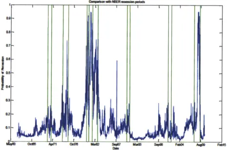
Figure 2. Comparison of predicted probabilities of recession with the NBER recession periods on a weekly basis FR8 I~~~~ & - L

~

~

---- 1 LO LB 3- 2-.1 ... ... - . ... ... .. --- --- --- ... ... ..---- -- -,- , --- - - --- - -- - " - - - - =--WAIV AqM

In the above figure the blue line depicts the probability of recession as generated from the model, while the regions specified by the green lines correspond to recession periods identified by NBER. It becomes clear that the model generates a probability of recession higher than 50% for four out of the seven major periods of recession, while for the remaining three periods it generates probabilities that are significantly

greater compared to the unconditional probability of recession.

The predicted weekly probabilities which indicate the probability of a recession occurring in the next quarter will be used in the next part for the estimation of the stock loadings on the recession factor.

ESTIMATION OF THE LOADINGS

General approach

After the estimation of the model which can predict the probability of recession in the next quarter, I

focus on the estimation of the loadings (betas) of the stocks on the changes in the recession factor. The

estimation of the betas is expected to produce a measure of the sensitivity of the stock returns to the

recession factor. A positive beta is an indication of a potential hedge (countercyclical stock) against this

factor as the returns of the stock seem to move towards the same direction with the changes in the

probability of recession. For example, positive returns are likely to occur when the probability of

recession increases compared to the previous observation. On the other hand, a negative beta is an

indication of a cyclical stock whose price is likely to decline with a rising probability of recession.

The beta estimations generated by the linear regression of the stock returns over the changes in the

probability of recession suffer from misestimation issues as the least-squares technique deals with the

properties of sample statistics given the true value of parameters. The situation here is the reverse as it is

the sample coefficient that is known and on the basis of this information we want to infer about the actual

distribution of the parameter. Another issue with the least-squares estimation of betas is the fact that it

does not take into account prior information regarding the characteristics of their distribution ignoring

information outside the sample information. In the case of beta estimation, prior information is of high

importance. This can be very well addressed using Vasicek's technique which minimizes the loss due to

misestimation, and takes into account knowledge of the prior distribution of the parameters.

Sample Construction

For the estimation of the stock loadings on the recession factor, stock return data are downloaded from the Center for Research in Security Prices (CRSP). The data include holding period returns for all the stocks that traded on the NYSE. AMEX and NASDAQ stock markets for the period of this analysis

(1962Q1-2010Q3). The total number of individual securities for which there are available data reached 24712,

providing a rich in terms of information dataset. Each stock is identified by its own permanent number (PERMNO) assigned to it by CRSP.

Methodology

At a first stage the betas are estimated on rolling five-year windows starting from 1962Q1 until 2010Q3 producing a series of 45 years of beta estimations. In order to proceed to the calculation of the loadings there is an additional provision of at least two years of available data. The betas are estimated using the least-squares method and for each of the estimations a number of statistical measures are calculated including t-statistics, p-values, and standard errors of the estimation.

At a second stage the estimated betas are adjusted using the Vasicek technique. The reasons for this adjustment, as well as the methodology employed are described in the following part.

Vasicek Betas

The least-squares technique employed in the estimation of betas consists of fitting a linear relationship between the rates of return on a stock and the percentages of the change in the probability of recession so that the sum of squared differences between the stock's actual observed returns and these implied by the assumptions for the distribution is minimized. The estimates generated are the best unbiased estimates of the parameters as the expected value of each of them is equal to the corresponding parameter and the standard error takes the minimal value. However, these criteria do not fully reflect the desired characteristics of a beta estimator. In the method of least-squares, there is an implicit assumption that the true value of the parameter is known. In reality, though, the sample coefficient is known and based on this information I desire to infer the distribution of the parameter.

In this case, the objective is an estimate that given the available sample information, the true beta will be below or above it with equal probability. Also, the knowledge of the cross-sectional distribution of betas can be used as prior information for the estimation of the stock loadings. This is captured via Vasicek's technique, which adjusts past betas towards the average beta by modifying each beta depending on the

sampling error about beta. When the sampling error is large, there is higher chance of larger difference from the average beta. Thus, lower weight will be given to betas with larger sampling error. This is summarized by the following formula:

2 2

/2 2 +2 +1h

+ +r

Where: A2 is the forecast of beta for stock i for period 2 (later period); ,- is the average beta across the

sample of stocks in period 1 (earlier period); 6% is the variance of the distribution of historical estimates of beta across the sample of stocks; ij; is the estimate of beta for stock i in period 1; 2 is the variance

of the estimate of beta for stock i in period 1.

In essence, this estimator which is derived from a Bayesian framework pulls

fa

towards the prior mean/h, with the degree depending upon the uncertainty about A relative to the spread in the prior distribution. The A2 posterior estimate of beta for stock i is preferred to the classical sampling-theory estimates because Bayesian procedures produce estimates that minimize the loss due to misestimation, while sampling-theory estimates focus on the minimization of the error of sampling. This is a result of the fact that Bayesian theory deals with the distribution of the parameters given the available information, while sampling theory deals with the properties of sample statistics given the true value of the parameters. Also, Bayesian theory weights the expected losses by a prior distribution of the parameters, thus incorporating knowledge which is available in addition to the sample information. This is particularly meaningful in the case of betas estimation, where prior information is usually sizeable.

RECESSION FACTOR AS RISK FACTOR

General approach

In this part of the analysis with the use of the Fama-MacBeth procedure for running cross-sectional regressions and calculating standard errors, I attempt to explore whether the change in the probability of recession is a risk factor exposure to which investors demand a risk premium. After regressing the cross-sectional Vasicek adjusted betas over the excess returns of the stocks for each one of the 44 years. and accounting for the standard errors, I identified the change in the probability of recession as a risk factor for which investors demand a risk premium.

Sample Construction

For the application of the Fama-MacBeth procedure, annual stock returns for the period of 1967Q1 to

2010Q4 are calculated from the compounded daily returns already downloaded from the Center for

Research in Security Prices (CRSP), the three-month Treasury Bill rate is retrieved on a annual basis from the St. Louis Federal Reserve database for the period of 1967Q1 to 2010Q. and the betas used in the cross-sectional regressions are the Vasicek adjusted betas already calculated from the previous section.

Methodology

The Fama - _{MacBeth procedure is employed to identify whether the recession factor is an actual risk} factor for which investors demand a risk preminum This procedure provides a framework for nmning cross-sectional regressions, and for producing standard errors and test statistics. The way this methodology was applied in the context of this analysis is summarized below.

" First, Vasicek adjusted loadings on the recession factor are estimated for each of the stocks with

sufficient amount of data, and for each of the 45 years of the analysis. Five-year rolling regressions are used to estimate the loadings and the Vasicek method is employed to obtain their adjusted values.

" Second, a cross-sectional regression is run for each time period. More specifically, for each of the 44

years (I drop a year from the original 45 as Vasicek adjusted betas are posterior estimates and there is no available information for stock returns during 2011), the factor ), is estimated from the cross-section (across the stocks 1,...,n) regression:

R=

Ai#i

+ Eit

Where: Rf are the annual excess stock returns calculated as the annual stock returns minus the annual observation of the three-month Treasury Bill rate;

fi

are the regressors (the Vasicek adjusted betas); i indicates the stock; t is an indication of time in years.

* Third, X and Eg are estimated as the average of the cross-sectional regression estimates

T:

The Fama - _{MacBeth procedure is a useful and simple technique for the analysis of data that have a} cross-sectional element as well as a time series element, like the ones in this analysis. Also, it allows for changing betas, something that cannot be easily handled in a single unconditional cross-sectional regression test. This procedure proposes running of a cross-sectional regression at each point in time,

averaging the cross-sectional At estimates to get an estimate of A, and the use of the time-series standard deviation of

At,

to estimate the standard error of

A.

Estimation Results, Discussion

The results of the regression of the excess stock returns over the stock beta estimates for each of the 44 time periods are summarized at table 2.

Table 2. Estimation of A and 95% confidence interval estimation

A 95% confidence interval

-6.563 -10.4383 -2.6876

The negative sign in the estimation results for X indicates that investors demand a risk premium in order to compensate for the exposure they have to the recession risk factor. More specifically, based on the estimation results when the exposure of a stock to the recession factor is positive (countercyclical stocks) investors appear to pay a risk premium for this hedge, while when the exposure of a stock to the recession factor is negative (cyclical stocks) investors appear to demand a risk premium for the exposure they take on this risk factor. In order to identify whether this risk factor is captured or not by the standard factors of the Fama - French Three Factor Model in a following part, I will construct portfolios with long positions on stocks with a high, and short positions on stocks with low loadings on the recession risk factor, the returns of which will be regressed over these three factors. If the constant of the regression occurs statistically significant, this will be an indication of a new risk factor completely unrelated to the other three. Otherwise, this will be an indication that this factor is captured by the three commonly used factors.

INDUSTRY ANALYSIS

General approach

At this point, the analysis is expanded to an industry level, where I attempt to identify patterns in several

industries in terms of their behavior regarding their exposure to recession risk factor. Based on Kenneth

French's industry classification of the SIC codes, each stock is assigned to a particular industry numbered

from 1 to 30. The stocks are sorted in an ascending order according to their Vasicek adjusted beta

loadings and they are arranged into deciles. For every industry I calculate its contribution in each one of

analysis over the number of the deciles it becomes obvious that across them there are industries which are

over-represented, while others are under-represented. More specifically, particular industries like food

products, household consumer goods, utilities, and telecommunications appear to be countercyclical,

while industries like clothing, textiles, and aircraft, ship and railroad equipment exhibit cyclicality

patterns. There is also a large number of industries that do not follow a particular pattern.

Data Specification

For the task of sorting the stocks into deciles based on the sensitivity on the recession factor, for each one

of the companies included in the analysis the downloaded data includes monthly observations of the

Standard Industrial Classification Code (SIC), the Closing Price or the Bid-Ask Average Price (PRC), and

the Number of Shares Outstanding (SHROUT). The data are retrieved from the CRSP database and

spanned from 1966Q1 to 2010Q4. For the classification of the companies into a smaller number of

industries, Kenneth French's 30 industry classification is employed.

Methodology

At a first stage the market capitalization of each stock is calculated on a yearly basis as the product of the

closing price and the number of shares outstanding. Also, each company is assigned an industry ID

ranging from 1 to 30 to match Kenneth French's industry classification. For each of the 45

time windows

the calculated betas are sorted in an ascending order and the stocks are assigned to deciles based on their

loadings. At the same time the industry ID and the company capitalization are assigned at the same decile

with the stock beta. For each of the created deciles and for the time span of the analysis, the industry

concentration is calculated as a percentage of the industry capitalization within the decile divided by the

total capitalization of the decile. Then, the intertemporal average industry concentration is calculated for

each of the deciles and for each of the industries.

The intertemporal average industry concentration for each of the deciles is normalized on an industry

basis by dividing each industry with the sum of this industry concentration at each decile. The normalized

industry concentration is regressed over the number of the deciles ranging from 1 to 10. Finally, principal

component analysis is applied on that dataset to identify particular data patterns.

Results and Discussion

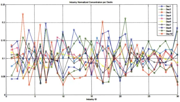
The plot of the intertemporal industry normalized concentration per decile is presented

in

Figure 2. From

this plot it is difficult to identify patterns and to draw conclusions regarding the over or under

representation of particular industries across deciles. Nevertheless, for particular industries like 1, 6, 7, 10,

17, and 30 there is an indication that the concentration on the deciles follows a pattern either increasing,

or decreasing with the number of the decile, indicating that the industries with the numbers 1, 6, 30 and

the ones with numbers 7, 10, 17 belong to the same group in terms of their sensitivity to the recession

factor.

Figure 3. Industry normalized concentration per decile

-xmf Hwnmz Cnmntim wD -e-o.7 0.2- --- o M-0-- ID --0- 0= I-1 w

scand aloeinerdtathfrsgou

has a higher concentration on the

higher

deciles (71-3).

whiigelenenrtino

thee

deciles (7-10) is an indication of industries which can be a potential hedge against recessions as their

returns are positively correlated to changes in the recession factor.

On

the other hand, a higher

concentration on the higher deciles is an indication that these industries show cyclicality thus suffering

from losses during periods of recession.

In order to obtain a clearer view regarding potential industry patterns in terms of sensitivity to recession

risk factor, principal component analysis is employed on the industry normalized contribution at each

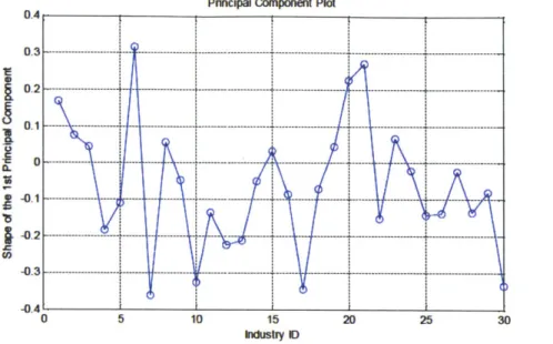
decile. The results are summarized on Figure 3.

Figure 4. Shape of the first principal component applied on the industry normalized contribution at each decile

Pnncipal Component Plot

10 15

idustby )

20 25 30

From the shape of the first principal component it becomes obvious that particular industries behave in a

completely different way. It is clear from the way data is fit that industries 1, 6, 20, and 21 show

completely the opposite behavior form the one industries 7, 10, 17, and 30 show, while for the remaining

industries a clear pattern cannot be identified. It is clear that in the deciles where the first group is

over-represented the other is under-over-represented, but nothing can be inferred for the level of the deciles (high or

low). In order to draw safe conclusions regarding the propensity of each of the two industry groups on the

recession risk factor a different approach is needed.

For each of the industries the normalized concentration in each of the deciles is regressed over the number

of the deciles, ranging from 1 to 10. The coefficients obtained from the regressions as well as useful

statistics are summarized on Table 3 and Figure 4.

--1--- - --- - - -- ---- - --- -- ----0.3 - -- ---- - --- - --- -4 --0.4 0

Table 3. Industry Coefficients on the number of deciles

ED Industry Coefficient Pvalue R_squared

1 Food Products 0.0088 0.0033 0.6807

2 Beer and Liquor 0.0037 0.2923 0.1371

3 Tobacco Products 0.0031 0.6390 0.0288

4 Recreation -0.0093 0.0445 0.4147

5 Printing and Publishing -0.0062 0.0265 0.4795 6 Household Consumer Goods 0.0166 0.0000 0.9261

7 Clothing -0.0184 0.0000 0.9255 8 Healthcare/Pharmaceutical 0.0030 0.2225 0.1795 9 Chemicals -0.0023 0.5831 0.0393 10 Textiles -0.0168 0.0001 0.8709 11 Construction/Constr. Materials -0.0070 0.0063 0.6278 12 Steel Works -0.0115 0.0003 0.8170 13 Fabricated Products/Machinery -0.0107 0.0001 0.8701 14 Electrical Equipment -0.0030 0.4326 0.0786 15 Automobiles and Trucks 0.0017 0.6421 0.0283 16 Aircraft, ship, and railroad equip. -0.0047 0.2110 0.1877

17 Mining -0.0182 0.0003 0.8156

18 Coal -0.0038 0.5082 0.0566

19 Pertoleum and Natural Gas 0.0021 0.1701 0.2212

20 Utilities 0.0116 0.0019 0.7221

21 Telecommunications 0.0134 0.0141 0.5500

22 Personal and Business serv. -0.0075 0.0217 0.5026 23 Business Equipment 0.0036 0.0633 0.3673

24 Business Supplies -0.0016 0.5104 0.0560

25 Transportation -0.0072 0.0016 0.7332

26 Wholesale -0.0072 0.0017 0.7276

27 Retail -0.0011 0.5914 0.0376

28 Restaurants, Hotels, Motels -0.0069 0.0117 0.5691

29 Financials -0.0041 0.0028 0.6925

30 Everything Else -0.0171 0.0000 0.8979

The highlighted lines indicate that the coefficients obtained are statistically significant at a level of

statistical significance of

5%

and the R

2

_{of the regression is greater than}

_55%.

Figure 5. Regression results of the intertermporal normalized industry concentration over the number of deciles ranging from 1 to 10, industry coeficients

Industr Coeficifnt 0.021 0.015--- 0.01--

.aO.005j-8

co 04- F-0.005- -0.01- -0.015--0.02 I_ _ _ _ _ _ _ _ _ 05 10 15 20) 25 30 hndusity ID

From the industry coefficients

it

becomes clear that the patterns identified from the principal component

analysis are still strong and that the shape of the industry coefficients plot is similar to the one obtained

from the shape of the first principal component. It also becomes obvious that the first group of industries

is over-represented in the high deciles, while the second is over-represented in the lower deciles. It is also

clear that the remaining industries do not show a particular pattern.

Industries that are over-represented in the high deciles are more likely to provide positive returns during

periods of recessions. Such industries include food products, household consumer goods, utilities, and

telecommunications. However, industries that are over-represented in the low deciles are more likely to

suffer from losses in periods of recessions. Such industries include clothing~ textiles, mining, and aircraft,

ship, and railroad equipment. The results are also intuitive as the first industry group is comprised of

companies whose products appear to have inelastic demand and thus their revenues are not expected to be

significantly affected by periods of recessions. On the other hand, the second industry group is comprised

of companies whose products exhibit elastic demand and as a result their revenues are highly correlated

with changes in the economic activity leading to significant declines in revenues during periods of

economic contraction.

ROBUSTNESS ANALYSIS, IMPLICATIONS

General approach

In this part of the analysis, a number of tests are conducted in order to ensure the stability of the loadings,

to identify the ex-post exposure of the stocks with high loadings on the recession risk factor, and to prove

whether the market over or underreacts to changes in recession risk.

Two different portfolios are formed based on the loading of the stocks to the risk factor. The loadings

have already been classified into deciles from the previous part. The first portfolio (full scale portfolio) is

consisted of long positions on the last decile (low exposure to recession risk) and of short positions on the

first decile (high exposure to recession risk). The second portfolio (within industry portfolio) contains

long positions on the last decile and short positions on the first decile, but here the deciles have been

calculated within each one of the industries. The rationale behind this construction is the elimination of

the industry element. Both portfolios are weighted on the capitalization of the companies included. The

excess returns of these portfolios are regressed over the factors of the Fama

-

French model and from the

following analysis it becomes clear that the first portfolio is tilted towards big companies with low book

to market ratio, while the second one does not show any particular relationship with these factors.

However, both portfolios appear to have statistically significant constant coefficient.

Furthermore, the calculated loadings from the previous parts are tested for their intertemporal stability.

The objective of this test is to prove that it is possible to construct a reliable hedge on the indicator of

recession risk. At a next step I attempt to answer the question whether stocks with high betas have lower

risk exposure ex-post. From the results of these tests it becomes clear that the calculated loadings are

stable over time showing an average ranking correlation of 80.1%, and that stocks with higher betas show

on average positive returns in periods of recessions.

Finally, to identify whether the stock market over or underreacts to changes in recession risk, for the

period of the analysis the returns of the full scale portfolio are regressed over the changes in risk factor

and particularly over the residuals of the AR(2) process on these changes. The residuals are used in order

to capture the new information that comes into market. The loading on the first lag of the residuals is

statistically significant indicating that the market underreacts to changes in recession risk and that

investors can benefit from holding these portfolios properly weighted on the residuals.

Data Specification

For the purposes of the analysis in this part. data for real GDP growth are downloaded from the St. Louis Federal Reserve database, while data for the Fama - French factors are downloaded from Kenneth French's online database. Finally, data regarding stock returns are retrieved from the CRSP database. The data include holding period returns for all the stocks that traded on the NYSE, AMEX and NASDAQ stock markets on a monthly basis for the period of this analysis (1966Q1- 2010Q3).

Methodology

The first of the two portfolios is formed by taking long positions on the stocks residing in the lowest decile and short positions on the ones residing in the highest decile. The components of this portfolio are weighed according to their market capitalization. For the construction of the second portfolio, in each one of the industries the stocks are sorted in an ascending order and deciles are formed. The first and the last decile are finally included in the portfolio. As with the first one, the stocks comprising the last decile are bought and the stocks comprising the first one are sold, while the weights are proportional to the company capitalization. For both portfolios the returns are calculated on a monthly basis and regressed over the Fama - French factors of the same period. All regressions are performed using the ordinary least square method and the T-stats are adjusted for heteroscedasticity using the Newey West method with a lag of 5.

For the beta stability test, Spearman's rank correlation coefficient is employed. The rank correlation is calculated for 44 consecutive periods. Also, to answer the question of whether stocks with high betas have lower recession exposure ex-post, the average returns of the first portfolio are calculated on two different cases. The first refers to periods with negative and the second to periods with positive real GDP growth. In order to conclude whether market fully appreciates that recessions are partly predictable, the portfolio returns are regressed over the contemporaneous as well as over the first lag of the residuals level estimated by applying an AR(2) process on the changes of the recession risk factor. The AR(2) process employed here is described below:

Aft

= ao + a1A.t-1 + a2At-x +#ft-1 + et

Where: Apit is the change in the level of the recession risk factor; ao, a,,a2,fl are the loadings on the

lagged time series of A 5; et are the residuals of the regression, and t represents the time in months. The residual weighted portfolio profits or losses are calculated by:

T

Profitt+ = _ResR+1

t=1

Where:

Restis

the residual level observed at the end of month

t; Rt is the return generated by the first

portfolio on month t+1.

Finally, for the residual weighted portfolios the information ratio is calculated as the ratio of the mean

profits or losses to the standard deviation of the profits or losses multiplied by the square root of 12

because the observations are in monthly terms.

Discussion, Results

Properties of the created portfolios

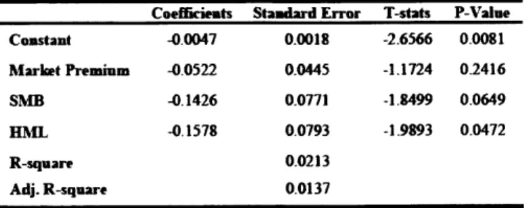
From the regression of the excess returns of the portfolios over the Fama - French factors it becomes clear that only a small fraction of the variability of the portfolios returns can be explained from these factors. Regarding the full scale portfolio it is evident that it has a negative exposure to low market capitalization and high book to market companies. This result is intuitive as most of the companies that belong to countercyclical industries share these traits. The relatively low adjusted R2 of the regression is an indication that the created portfolio has risk exposures that cannot be fully captured by the standard factors of the Fama - French model. Nevertheless, the constant coefficient appears to be strongly statistically significant, indicating the existence of another risk factor. It also has a negative loading which implies that investors pay a premium for recession risk protection. The regression results for the first portfolio are summarized on table 4.

Table 4. Regression of full scale portfolio excess returns over Fama -French factors

Coeffieents Standard Error T-stats P-Value

Constant -O.0047 0.0018 -2.6566 0.0081 Market Premium -0.0522 0.0445 -1.1724 02416 SMB -0.1426 0.0771 -1.8499 0.0649 HML -0.1578 0.0793 -1.9893 0.0472 R-square 0.0213 Adj. R-square 0.0137

From the regression of the excess returns of the within industry portfolio over the Fama - French factors it can be easily inferred that these factors are not suitable to explain the variability of the portfolio returns. None of the factors appeared statistically significant, but the constant coefficient appears again negatively

statistically significant. The results of the regression analysis for the second portfolio are summarized on table 5.

Table 5. _{Regression of within industry portfolio excess returns over Fama} -French factors

Coefficients Standard Error T-stats P-Value

Constant -0.0043 0.0015 -2.8180 0.0050 Market Premium -0.0213 0.0331 -0.6426 0.5208 SMB -0.0362 0.0522 -0.6932 0.4885 HML -0.0643 0.0584 -1-1014 0.2712 R-square 0.0042 Adj. R-square -0.0015

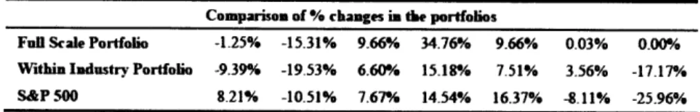
Comparing the returns of each of the portfolios to the returns of the market (S&P 500) it can easily be inferred that the full scale portfolio tends to produce higher returns during recessions compared to the ones generated by the within industry one. It becomes clear that in the within industry portfolio protection deteriorates as a result of the inclusion of companies from all the industries. This could be due to the enclosure of small companies as some of the industries contain a large number of them. Also, the first portfolio seems to provide a 'safety net' during most of recession periods as its returns tend to be higher compared to the ones of the market. The comparison results are summarized on table 6.

Table 6. Comparison of % changes in the portfolios during periods of recessions

Comparison of % changes in the portfolios

Ful Scale Portfolio -1.25% -15.31% 9.66% 34.76% 9.66% 0.03% 0.00% Within Industry Portfolio -9.39% -19.53% 6.60% 15.18% 7.51% 3.56% -17.17%

S&P 500 8.21% -10.51% 7.67% 14.54% 16.37% -8.11% -25.96%

Beta stability

The calculated betas from the previous parts are tested for their intertemporal stability. Spearman's rank

correlation coefficient is the rank correlation measure employed in this analysis. The average rank

correlation of the loadings is equal to 81.01% indicating that betas are stable over time and that portfolios

constructed on the ranking of the loadings are a reliable hedge against recession risk.

Consistency of the procedure

In order to conclude on the consistency of the procedure, the average quarterly return of the full scale

growth. The average quarterly return during periods of economic downturn is equal to 3.89%, while the

average quarterly return during periods of economic growth is equal to -1.02%. The

t

statistic of the test

for equality of the two average returns is 2.59 suggesting that the initial hypothesis of equality is rejected

at a level of confidence of 1%. This is a clear indication that stocks with high loadings on the risk factor

have lower recession exposure ex-post. This finding also validates the consistency of the procedure and

confirms that the performance of such a portfolio during recessions is significantly increased.

Recession portfolio performance

The monthly returns of the full scale portfolio, which is rebalanced on a yearly basis by taking long

positions on the last decile and short positions on the first decile of the beta sorted stocks, are regressed

over the contemporaneous and first lagged levels of the residuals estimated from the AR(2) process. From

the results of the regression it is clear that the coefficient of the first lagged level of the estimated

residuals is statistically significant. This is an indication that the market does not fully appreciate that

recessions are partly predictable, and that it is possible to create a portfolio which can benefit from this

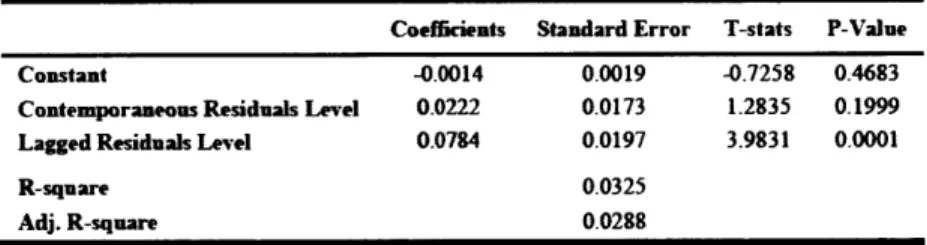
market behavior. The results of the regression are summarized on table 7.

Table 7. Regression of full scale portfolio returns over contemporaneous and first lagged residuals levels

Coefficients Standard Error T-stats P-Value

Constant -0.0014 0.0019 -0.7258 0.4683

Contemporaneous Residuals Level 0.0222 0.0173 1.2835 0.1999

Lagged Residuals Level 0.0784 0.0197 3.9831 0.0001

R-square 0.0325

Adj. R-square 0.0288

The regression results provide useful insight in terms of market appreciation of changes in recession risk.

It is possible that a portfolio could be constructed, which could produce significant profits by taking into

advantage the lagged incorporation of changes in recession risk from the market. For the purposes of this

analysis, the portfolios already constructed constitute the basis of this proposed new portfolio. The

exposure of this portfolio to the initial ones is proportional to the lagged residuals level. More

specifically, a positive level of the first lag of residuals provides a buy signal, while a negative generates

sales. The amount by which the portfolio is bought or sold is directly proportional to the levels of the

lagged residuals. It becomes clear fromfigure 6 that such a portfolio can generate significant returns.

Figure 6. Comparison of porfollo profit-loss with NBER periods of recession

Lmnpason wnnU1 Pan-'enoos or Iecession

Mar82 Sep87 Mar93 Sep98

Date Feb04 Aug09 Feb15

From figure 7

_{it becomes evident how portfolio weights based on the lagged residuals level lead to a}

significant appreciation of the portfolio value. It can be easily observed that the trading strategy based on

the levels of residuals takes the right position most of the time leading to an exceptional performance with

the annualized information ratio of the strategy being equal to 6.0191. It is also clear that the level of

lagged residuals captures very well the exposure that the portfolio should have in periods with increased

probability of recession. It can also be observed that low levels of the lagged residuals lead to small

positions, and that high levels trigger big positions in the scale portfolio.

Figure 7. Joint plot of the first

lag

of the residuals level and profit-loss from the proportional exposure to full scale portfolio

'D1

Jait Pat d Lal Resids and Pct.LAs of the Expoums to FM Sed ParDio

I I I LDA m~e 0.2 04 _05 01 1- _Cdi -_ApTI I I I I 1 1 14

CAM Ii d S."7 UM9 Sipl F0d4 Ao FOMS

GDi 0.3-0.25k 021- 0.15[- 0.1- 0.05-Cc65 Apr7l Oct76 M.3

-d

In order to support the above results and the finding that market does not fully appreciate that recessions

are partly predictable I constructed an alternative portfolio based again on the full scale portfolio of the

analysis with weights dictated by the levels of the second lag of the estimated residuals level. It is evident

from figure

8

that such a portfolio is capable of generating significantly positive performance during the

period of the analysis. However, the return generated by this trading strategy is to a large extent lower

compared to the return of the previous strategy. This finding is an indication of the robustness of the

procedure and is broadly in line with the beta stability identified above.

Figure 8. Comparison of alternative portfolio levels with NBER periods of recession

Compadson th IEER Pedlods of Recession

0.08- 0.06- 0.04-0.02 --0.02k -0 6 I1 -. I O I I Sep7

A4Wr1 Oct76 MaM2 Sep07

Date

Mai93 Sep98 Feb04

In order to get a better sense of the underlying dynamics of this alternative portfolio the full scale

portfolio is decomposed to its long and short component. For each of the components I calculate the

profits and losses based on the exposure dictated by the lagged residuals level. The profits and losses of

the exposure to the components of the full scale portfolio are summarized onfigure

9

andfigure

10.

-ffi~

Figure 9. Joint plot of lagged residuals and profit-loss of the long position component of the full scale portfolio

Ja* Plit d Lggd Rieskkis and PMwtLces d Lang POslMn d Fd Scae PatkIo

2

DFe

Figure 10. Joint plot of lagged residuals and profit-loss, of the short position component of full scale portfolio

It can be easily observed from the figures above that the main contributor in the performance of the

alternative portfolio is the short position component of the full scale portfolio. This raises concerns

because the short position may not be available at the time it is needed, and also it comes with a cost, but

the fact that the constructed portfolios are market weighted alleviates this concern as the largest and most

liquid stocks have a higher contribution to these portfolios.

At this point it would be interesting to explore the performance of a second alternative portfolio based on

the within industry portfolio and the lagged residuals level. As with the previous case, the exposure to the

within industry portfolio is determined by the level of the lagged residuals. This trading strategy also

exhibits significant performance, but it is lower compared to the one achieved by the first alternative

portfolio. The annualized information ratio of this strategy is 5.8026. The profits and losses of this

strategy, as well as the lagged residuals levels are depicted onfigure

11.

Figure 11. Joint plot of lagged residuals and profit-loss of the residual weighted exposure to within industry

portfolio

ais[-aOsF

.hit PitI d Lgge Fbufitfa u nea*N-of ftw Expoiue to Win iknmby Pantio

02i i L I I I t laa

05 1 7 5 M0-8..

As with before the within industry portfolio is decomposed to the long position and the short position

component. Both components are weighted on the lagged residuals level and their behavior is similar to

the one the full scale portfolio components exhibited above. The short position contributes the most to the

profitability of the strategy, while the long is consistently in a negative territory. This is apparent from