HAL Id: hal-03021075
https://hal.inria.fr/hal-03021075
Submitted on 24 Nov 2020
HAL is a multi-disciplinary open access
archive for the deposit and dissemination of
sci-entific research documents, whether they are
pub-lished or not. The documents may come from
teaching and research institutions in France or
abroad, or from public or private research centers.
L’archive ouverte pluridisciplinaire HAL, est
destinée au dépôt et à la diffusion de documents
scientifiques de niveau recherche, publiés ou non,
émanant des établissements d’enseignement et de
recherche français ou étrangers, des laboratoires
publics ou privés.
A Question Answering System For Interacting with
SDMX Databases
Guillaume Thiry, Ioana Manolescu, Leo Liberti
To cite this version:
Guillaume Thiry, Ioana Manolescu, Leo Liberti. A Question Answering System For Interacting with
SDMX Databases. NLIWOD 2020 - 6th Natural Language Interfaces for the Web of Data / Workshop
(in conjunction with ISWC), Nov 2020, Heraklion, Greece. �hal-03021075�
with SDMX Databases
Guillaume Thiry1,2, Ioana Manolescu2,1, and Leo Liberti3,1
1
Institut Polytechnique de Paris [email protected] 2Inria [email protected]3CNRS
Abstract. Among existing sources of Open Data, statistical databases published by national and international organizations such as the Inter-national Monetary Fund, the United Nations, OECD etc. stand out for their high quality and valuable insights. However, technical means to interact easily with such sources are currently lacking.
This article presents an effort to build an interactive Question Answering system for accessing statistical databases structured according to the SDMX (Statistical Data and Metadata Exchange) standard promoted by the abovementioned institutions. We describe the system architectures, its main technical choices, and present a preliminary evaluation. The system is available online.
Keywords: statistical databases · Question Answering · SDMX
1
Introduction
Open Data has the potential of enabling societal changes of significant impact. On the one hand, the availability of data allows the creation of innovative prod-ucts and applications. On the other hand, data that documents various aspects of a societal functioning is a crucial ingredient for its self-understanding, and it enables citizens to make informed choices, from personal consumer decisions to voting in elections. Such statistical databases are also valuable as references to be used in fact-checking [7]. Indeed, claims about statistical quantities such as unemployment or immigration figures are a hot topic of political debate in many countries.
Statistical databases published by national and international institutions such as the United Nations (UN), the Organisation for Economic Co-operation and Development (OECD), the International Monetary Fund (IMF), EuroStat, etc. stand out among Open Data sources for the quality and comprehensive-ness of their data, gathered at a significant expense of qualified personnel and carefully curated, structured and organized. To enable interoperability among their data sources, these and other organizations have established a standard
Copyright c 2020 for this paper by its authors. Use permitted under Creative Com-mons License Attribution 4.0 International (CC BY 4.0).
Dataflow Data Structure Definition
Constraints Categorisation
Category Schemes
Accepted values for each dimension
List of the dimensions and the attributes of the table Dimension 1 ...
Concept Codelist
SDMX Data
SDMX Metadata
Description of each cell of the dataset (dimensions + value)
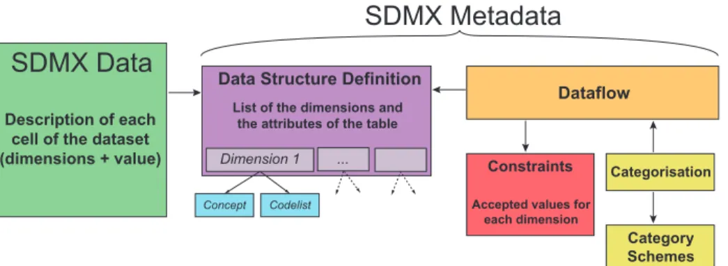
Fig. 1. SDMX data organisation.
for describing their statistical data, named SDMX (Statistical Data and Meta-data eXchange) [1]. The standard specification describes the various elements involved in specifying the (mostly numerical) data, and in describing it accord-ing to the relevant dimensions. Several institutions have adopted the standard, and published Web sites online with data sheets together with textual descrip-tions and sometimes automated visualization means for human users to interact with the data. As an example on which we build our presentation, we used the data and metadata provided by OECD, our partner, through its Web Service: http://de-staging-oecd.redpelicans.com/.
As this example shows, currently, interaction with an SDMX dataset takes the following form. (i) Users locate one or more pages on the Internet hosting the dataset(s) they are interested in; (ii) Users read the descriptions to check the expected content and semantics; (iii) they visualize the numerical data, possibly with the help of the visualization tools included in the pages.
Discussions with OECD experts working on Smart Data Practices and Solu-tions highlighted that this current usage scenario suffers from several limitaSolu-tions. First, searching for the right dataset is not easy, when multiple datasets may con-tain interesting answers, or when users’ terms specifying their question(s) do not match those used by statisticians describing their data. Second, having to face tables of numbers may be cumbersome for users interested in point queries, e.g., “what is the unemployment rate in Spain in Q3 of 2018?” Third, this scenario gives no support for more advanced queries of the form “where is unemployment higher than in Spain, in Q3 of 2018?”
Motivated by this observation, we have developed a tool which allows users to interact in an easier, more natural manner with SDMX statistical databases, by means of a QA system. In the remainder of the paper, we describe the SDMX standard (Section 2), before delving into our contribution: an architecture and algorithms for an interactive, English-speaking agent allowing natural language interaction with SDMX databases (Section 3 to Section 6). We present an eval-uation in Section 7, before discussing related work and concluding.
2
The SDMX standard
The SDMX standard enables the description of: statistical data (typically under the form of a multidimensional array whose cells contain numbers, e.g., sales
volume or percentage of people unemployed), and metadata, that is, the set of dimensions characterizing the data, as well as the values that these dimensions actually take in the data. Sample dimensions are for instance geographic (what area does a certain statistic correspond to), temporal (time period) or more specific to the data being described, e.g., tourist stays in a certain area can be split in hotel stays, bed-and-breakfast stays, and camping stays.
Concretely, SDMX advocates representing both data and metadata in XML1, a self-describing syntax which has several advantages. First, it lends itself easily to publishing data sets online, since XML can be easily turned into a Web page with the help of a style sheet. Second, XML is the syntax favored by Web ser-vice technologies such as SOAP [18] (for message exchange) and WSDL [19] (for Web service communications). This simplifies the implementation of an SDMX endpoint which allows querying an SDMX database (or repository) remotely, through a Web service client application.
The SDMX metadata is split into several parts, each of them describing one specific aspect of the data. These different pieces point to each other, as well as interact with the data, which could not be readable without its metadata. An overview of the design of the SDMX standard is given in Figure 1.
Data are organized in data tables which consist of cells. Each cell corre-sponds to a combination of values along each dimension present in the data table; each cell contains a numerical value (in green in the figure). A data table points to its metadata description, which is necessary in order to interpret its content. Specifically, the data table points to a Data Structure Definition (DSD), which is the central piece of the metadata architecture (in purple in the figure). The DSD lists the different dimensions used for this dataset, and attaches to each dimension a concept and a codelist (in blue in the figure). The concept gives more details about the dimension (an explicit name and a description) while the codelist is a dictionary that can be used to decode information about this dimension. For instance, the codelist of the dimension AREA may contain the pair “AU” = “AUSTRALIA” to state that “AU” may be used as a dimension value to denote “Australia” compactly. The DSD also lists other characteristics of the table, for instance whether its values are predicted, estimated, or actually computed.
Other important metadata components are the Constraints (in red) and the Categorisation (yellow). The Constraints specify the legal values for each dimen-sion of the table, to guarantee the integrity of the dataset. The Categorisation characterizes the way in which the data is classified within the Web Service that makes it available to users. For example, the table “Domestic tourism” is found in the category “Tourism”, itself a subcategory of “Industry”. These two parts are ultimately linked to the DSD via a part called the Dataflow (orange).
The SDMX metadata comprises more fields, for example some which are designed to ensure the proper construction of the data sets themselves etc. The
1
XML being the main standard, it is however useful to note that SDMX is also compatible with JSON and CSV
OECD Web Service
Parsers User
Generic information extractors Specific information
extractors
Grammatical Structure Dependency Structure Named Entity Recognition
Dates Type of sentence Comparisons & Aggregations Locations Main topic Other dimensions
Query Ask for more precision
Fill the request
SDMX Metadata SDMX Data Keywords dictionaries Keywords extraction Distance computing Request filler - Table to select - Dimension values - Comparisons - Aggregations Data Extractor Complete Request Data Extraction REST API Display the results
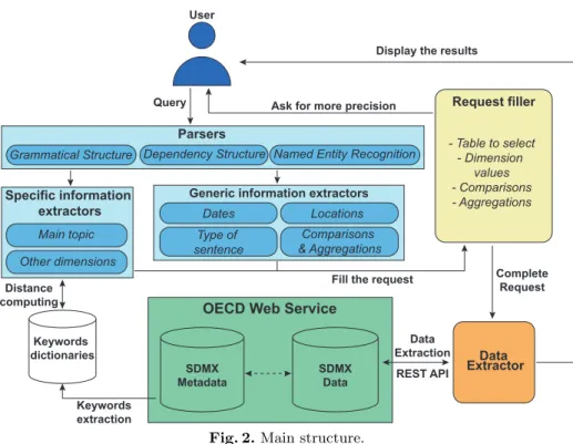
Fig. 2. Main structure.
modules mentioned above are those that we exploit for building our system, assuming that the data is correctly organized and described.
3
System overview
The main problem addressed by our QA agent is to understand information requests, when expressed in natural language. A typical question we aim at an-swering is: “What was the population of Japan in 2010?” A successful interaction with the system, thus, is a sequence in which a query was asked in natural lan-guage, understood correctly by the algorithm, and answered through appropriate queries on the SDMX data.
Our QA system is implemented in Python, based on the nltk toolkit and parsers from the Stanford NLP Group. It consists of 12 files and about 1800 lines of code; it is available online at https://github.com/guillaume-thiry/OECD-Chatbot. The general analysis pipeline, outlined in Figure 2, is as follows.
First, the user query, a natural language sentence, is analyzed by three differ-ent parsers, each gathering specific information from the query. A lexical parser assigns to each word a Part Of Speech (POS) Tag and captures how they form grammatical groups (such as a Noun Phrase [NP] or a Prepositional Phrase [PP]). The dependency parser identifies connections between non-consecutive words. These two first parsers are supplied by the Stanford CoreNLP toolkit [12] (interfacing with nltk). Lastly, a Named Entity Recognition (NER) parser rec-ognizes specific entities such as dates or places; we rely on the Stanford NER
module [8]. The results of these parsers are then used as input for different analysis functions (see below).
From the nature of SDMX data it follows that we expect user’s input to be questions concerning a statistical measure over one or more countries, at a given time. We have therefore implemented functions to extract dimensions such as the location(s) and date(s) from the phrase, when present; a separate module is tasked with understanding the type of the question asked. These modules are described more specifically in Section 4.
Concerning the query type (or structure), beyond direct questions asking for the value of a certain metric in a certain time and place, we also considered questions featuring comparisons, e.g., “Countries with more than 100 M inhab-itants”, and aggregation, e.g., “What are the five largest countries in term of GDP per capita ?”. The words used in such questions are relatively few and easy to detect (“more”, “less”, “higher”, “than”, “above” ...). However, because the syntactic structure of such questions is inherently more complex than that of simple questions, detecting and properly handling such structure is slightly more complex than understanding simple dimensions (date, place) in direct questions. We detail this in Section 5.
Last but not least, each question refers to a specific topic, e.g., unemployment rate, public debt or health investments, and specific dimensions, e.g., a question about a metric defined on the general population can be accompanied by a qual-ifier that restricts the questions to males or females. That depends on the user’s information needs. This part of the question would naturally change depending on the content of the database and the user interest; a generic approach needs to be taken for understanding it, based on the known metadata of the SDMX endpoint behind the system. This is discussed in Section 6.
Once all these questions have been answered by the different parts of our algorithm (with potentially some requests of precision addressed to the user), a final section of the system uses the SDMX REST API to get the correct table with the correct dimensions, applies potential comparisons and aggregations, and displays the answer in a appropriate way (a list, a graph, a map ...).
4
Understanding general dimensions of user questions
We discuss here the first steps for analysing the question: what is the quantity of interest to the user, and (if specified), in which time frame, and in which spatial location? Each of these tasks is handled by a specific module as explained below. Assumptions on the grammatical structure. We decided to focus on two very common question forms. First, the so-called WH-questions, such as “What is the population of Russia in 2012 ?”, include an explicit question in-dicator such as “Who”, “What” etc. Second, we also consider Nominal Phrase questions, e.g., “French GDP per capita”. Other questions types exist, such as Yes/No questions, or imperative statements (“Give me the surface of Peru”); in the current project state, these are not tackled, although we believe the extension would be quite easy.
We identify the question form based on the grammatical structure given by the parsers: a WH question usually corresponds to a WH Noun Phrase (WHNP, in short), while a nominal question is specified through a Nominal Phrase (NP). The question form can be used to determine the type of result the user wants. We have identified three main types of result: (i) The user could ask for the value of a specific metric or statistic, e.g., “What is the employment rate in Canada ?”. In such questions, the geographical area (e.g., Canada) and the time associated to the query metric may or may not be present. (ii) Users can ask for one or more geographical areas, e.g., “Largest nations of the world”. (iii) Users can ask for one or more time periods, e.g., “How many years with more unemployment than 2014”.
We detect those, depending on the structure, by looking for specific words. For instance, a WH question is signaled by the presence of a specific WH word; a geographical question is signaled by a “where”, and a set of time periods by a “when”. Finally, if the WH-word is “what”, we need to identify the word con-nected to it: “what” in conjunction with “countries” has a different meaning than when used with “population”. This connection is captured by the dependency parser. While these two question shapes do not exhaust the set of possibilities, they are those that occur most frequently in real-world journalistic fact-checks, as noted for instance in [5].
Time search. Time is a central dimension characterizing statistical data. We implemented a function that detects time questions at the granularity of the year, since this appeared sufficient for the SDMX data we used. This could be easily extended to quarter or month granularity. Our function is also capable of understanding time intervals such as “from 1930 to 1950” or “since 1950”. We can also detect time expressions such as “nowadays” or “over the last 10 years”. We rely on the NER component to signal DATE occurrences in the text. For instance, 1950 is tagged by the NER in all the sample occurrences mentioned above. However, NER does not capture the other qualifiers such as “from... to” or “since”, which are important to correctly understand the question. Therefore, after identifying a year such as “1950” in a sentence, we examine the Preposi-tional Phrase [PP] (in the grammatical structure) containing it. In this PP, we consider specific words such as “since”, “till” or “between” to know the meaning of that year. It is crucial to focus only on the PP of “1950” because words such as “since” can appear elsewhere in the sentence, even near “1950”, without having any relation with it.
Based on this analysis, we fill two parameters, FROM DATE and TO DATE, specifying the time period of interest for the user. We also keep a variable THAN DATE in memory, for the specific case of a year linked with the word “than”. This can be useful when working with comparisons, as we explain in Section 5.
Locations search. Another essential information for our statistical data is the location. The granularity adopted by most of the international organizations using SDMX is that of the countries, and that is our choice as well. This could be easily refined to regions or cities.
Experimenting with the NER component has shown that it is not suffi-ciently powerful in identifying occurrences of countries. Specifically, problems were raised by abbreviations such as “USA” or “UK” and with adjectives de-noting countries, such as “French”, “Finnish” etc. Instead, we created a set of dictionaries containing every country, with the corresponding adjectives and their multiple spellings. To achieve this, we took the list of member states from the UN website, and obtained the related linguistic information (abbreviations, alternative spellings, adjectival forms) from the Wikipedia pages of each country in the list. Another dictionary contains the names of several regions of the world with the corresponding countries, under the UN M49 standard2. This enables us to correctly understand expressions like “Western Europe” or “Latin America” and know exactly what countries are concerned.
Once countries or regions have been detected in the sentence, we analyze the context in the same way as for the dates. This enables us to correctly handle questions over statistical metrics between two countries, e.g., tourism or trade “from country A to country B”. These are detected by examining the contextual words in the PP of each country.
5
Understanding advanced search criteria
Comparisons and aggregations are the next more complex class of queries we consider; they occur quite naturally, even if not as often as the simpler queries discussed above. Typical examples are the questions “Countries with more than ...”, “Five countries with most ...” Such comparisons and aggregations are also basic features of database languages, such as SQL. We therefore decided to enhance the QA agent with the ability to handle them too.
Comparisons. We detect comparison questions that satisfy one of the structural patterns described below.
First, we look for a comparative adjective that can be specified by one word (e.g., “larger”) or two words (e.g., “more populous”), followed by the word “than”. This form is easy to detect, as the words expressing the exact com-parison (“more”, “less”, “richer”, “higher” etc.) are identified by a specific POS tag, and the word “than” is only used in English to signal such comparisons. We only need to verify that all the words that are necessary to form a correct comparative question are present and placed correctly in the sentence. If the word “than” is missing or appears in a position that does not correspond to the pattern, we do not recognize the question (thus we can ask for a reformulation of the query).
Second, in the specific case of a comparison with a numerical value (that we name threshold below), one can use words like “over” or “below”, e.g., “What countries have a population below 50 M”. A difficulty raised by these words is that they can appear in other contexts in a sentence. For instance, in the time-related expression “over the last 5 years”, the word “over” does not contribute to expressing a comparison. To avoid such confusions, every time one of these words appears, we check if it is linked to a numerical value and if this value is
2
not already interpreted as a date. If so, we consider that the sentence expresses a comparison, and the numerical value is the threshold.
Multiple comparisons in a phrase Next, we extended the algorithm to also handle multiple comparisons. Our system tries to split the sentence in as many clauses as there are comparisons, each one of them containing one comparison only; the splitting is based on separative words such as “and”, “but” or “while”. Therefore, a sentence like “Countries with a population above 10 M but below 50 M in 2012” is split into two clauses: “Countries with a population above 10 M” and “below 50 M in 2012”. This separation is only used to interpret each comparison properly: the other functions, such as for the detection of the time (“2012” here), are applied to the whole sentence.
Each clause thus extracted falls in one of the following three cases:
– Comparison with a threshold (discussed above). If the comparative structure uses “above” or “under” for example, we check the threshold as explained before. If it uses “more ... than”, then we search for the threshold after “than”. Observe that the function detecting the thresholds also looks for multiples like “M” (millions) or “bn” (billions) attached to the numbers. At the end, we know the exact value involved in the comparison.
– Comparison with a country or a year, e.g., “What countries have a higher GDP than Spain ?” Answering this requires the comparison of the GDP value for each country with the Spanish one. The same can happen with a list of years. This is the reason why we had a “THAN” category when looking for countries and years (Section 4). In such cases, we know that the user asks for a list of countries, and we know that a comparison is made, therefore we check in the detected countries of the sentence if one of them was linked to the word “than”. If so, we know that the comparison is of this country against all the others.
– Otherwise, we consider that two different values of the table are com-pared, e.g., “Countries with more male population than female population” or “Countries with less population in 2020 than in 1990”. In such cases, we inspect the phrase before and after the word “than” to determine what the two values compared are. This is performed on different levels, such as when filling the dimensions of the table (see Section 6), as a dimension can have one value before “than” and another “after”.
Aggregations Such patterns are easier to handle than the comparisons, because there are fewer possible variations in the respective linguistic structures. We are able to detect three ways to aggregate a list of countries or of years: through counting, maximum and minimum. Counting queries, such as “How many countries have ...”, can already be detected when analyzing the type of sentence (Section 4), as we have to treat structures like “How many” or “Number of” and inspect the sequel of the phrase to determine the type of information wanted: “How many countries ...” aims at measuring a list of countries, while “How many inhabitants ...” aims at a value. We detect queries interested in a maximum (or minimum) through the presence of certain words like superlatives (“highest”, “biggest”, “most” ...) or a few other specific words (“maximum”,
Case Score Case Score Equal stems 1 WordNet hyponym or hypernym 0.6 WordNet synonyms 1 Word2vec similary s with s > 0.2 s WordNet noun-adjective relation 0.7 None 0
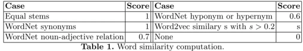
Table 1. Word similarity computation.
“top”, ...). Subsequently, the algorithm checks if a number is linked to this word, as it would indicate the number of items the user wants to see (“Best 5 countries ...”, “Top 10 highest ...”). If no such number is found, a default value is used: 1 if the word is singular (“Country with highest ...”) and 10 otherwise. This analysis outputs: if an aggregation was found; and, if yes, whether it is a maximum or minimum, and the number of items to return.
6
Understanding the question topic and dimensions
While we described above a set of methods for identifying some query elements specific to the kind of question, we now explain how we detect question topics. Specifically, we aim at answering the question “Which dataset should we use to answer this query?”.
Find the topic. Before looking for more details in the query, we have to determine the general topic of the query. Indeed, the details highly depend on the topic: if the query is about “population”, we may have to identify “male” or “female” as categories, but these do not apply if the query is about the “GDP”. For each table, we build a set of keywords using the SDMX metadata. We do the same for the query, removing query words that are too generic (e.g., “country”) or stop words (such as “in”, “to”, “with” etc.). Next, we compute a proximity score between the words of the query and the set of words corresponding to each table, in order to determine the tables most related to the query.
Our proximity function compares the stems of the input words, and finds their proximity according to word2vec [13] and WordNet [14]. We consider a set of different cases, shown in Table 1; to each there corresponds a certain similarity score. When two cases hold simultaneously, the higher similarity is kept.
To calculate the proximity between the query and a given table, we sum the proximity of each meaningful query word with the keywords of the table. Keywords characterizing a table can be found in four different places in the table metadata. Depending on the position, we give them different weights in the proximity computation formula, as shown in Table 2. [These weights were found by hand through trial and error; a Machine Learning approach could be used instead to learn their values] Finally, the proximity between a query and a table is computed as:
prox(query, table) = X q∈QueryWords
max
t∈TableWordsprox(q, t) weight(t) (1) Once we are able to compute the proximity score between our query and a given table, we can rank the tables according to their scores to find the most relevant ones. As shown in Section 7, this technique is not perfect, as some tables are very similar. The table with the highest proximity score may not always be
Name Details Weight Example Title Table title keywords 1 population Description Description keywords if any 0.6 number, inhabitants Dimensions Dimension name/value keywords 0.6 sex, female, male
Categories Table category name keywords 0.6 society, demography Table 2. Query-table similarity computation.
the most relevant one to answer the question. The solution we have found is to display a list of the tables with the highest scores to the user for him to choose. Indeed, the correct table usually belongs to this list in practice.
Filling the dimensions. Our last task is to detect possible dimension values in the user query, that is, e.g., “women” in the question “Number of French women”. Given a table that we identified as described above and which could contain relevant query results (for instance, a table about “French population”), we compute, for each dimension of the table and each value of a dimension, a proximity score between the query’s useful words and the name of the value. For each dimension, the value name most similar to the query keywords is finally retained, if the similarity is above a certain threshold. In our example, the query’s useful words are “French” and “women” and the table has a dimension “sex” with two values “male” and “female”. Because the similarity between “women” and “male” is lower than between “women” and “female”, the dimension “sex” gets the value “female”.
If, for a given dimension, no value is close enough to the query, three cases are possible. (i) If the dimension has only one value (e.g., “FREQUENCY” has “ANNUAL” as its only value in many SDMX datasets), this is systematically the default value. (ii) The default value can be the “total” value, as this is quite frequent in the data (“SEX” has “MALE”, “FEMALE” and “TOTAL” as values). (iii) Otherwise, no default value is identified, and the user is presented the possible values for the dimension in order to clarify the request. In our example, if the table also has a dimension “age” (with values “0-20 years old”, “20-40 years old” ...), no value is close enough, and “total” is used instead.
7
Experimental evaluation
Below, we describe qualitative evaluation results on each of the modules we developed and described above. Some of these (in particular those described in Section 6) can only be evaluated on an actual dataset; it should be noted that the only SDMX endpoint we had access to during this work (mentioned in Section 3) had relatively little data. Some others (e.g., detecting the question type, or extracting the time interval etc.) can be evaluated independently of an actual SDMX endpoint. All the queries used in the evaluation are available in the Github deposit of our code.
To perform our tests, we wrote for every module a set of test cases (queries) that we strived to make as realistic as possible, and also to highlight the capa-bilities and limitations of our approach. For each query, we manually specified the expected results, then we ran our code and measured how many correct re-sults we obtained. Some query topics come from the available OECD data; the
Categories Tables
Domestic Tourism Industry Inbound Tourism
[IND] Employment in tourism Key tourism indicators Open govt data
Government Public finance and economics
[GOV] Structure of govt expenditures by function and govt type Structure of govt investment by function
Enrolment by field Education Educational attainment
[EDU] Enrol by gender, program orientation and mode of study Enrolment by age
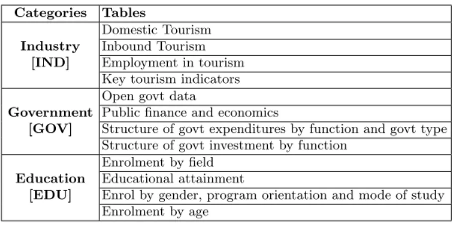
Table 3. OECD datasets used in our tests.
other topics are mainly taken from the “most popular tables” section of Euro-stat3. Overall, the queries cover 20 to 30 topics. To test topic and dimension extraction, we had to write queries related to the tables for which we had actual metadata. Using the available OECD Web service, we selected 12 tables over 3 different categories (outlined in Table 3) as targets of our queries.
Detecting question type To test this, we created a set of 100 queries, half of which are WH-questions while the other half are Nominal Phrases (NP). These queries were asking for a value, a list of countries or a list of years. Half of them also contained comparisons or aggregations. We assessed the precision of four query understanding tasks: finding the sentence type (WH or NP), un-derstanding the kind of result wanted (Value/Countries/Years), and detecting comparisons and aggregations. The result are as follows:
Parameter Accuracy Parameter Accuracy
Type of sentence 100% Comparison 97%
Return 94% Aggregation 94%
It is interesting to see where the algorithm failed and why: in our case, this is due to our linguistic patterns not being flexible enough. For example, in the sentence “Highest mortality rate before 40 years in the world”, the code falsely detects, based on “highest” and “years”, that we seek an aggregation over a list of years. Another example is the query “What is the minimum wage in Canada ?” because here “minimum” does not indicate an aggregation but belongs to the expression “minimum wage”. While these errors point to possible avenues for improvement, the accuracy results are already quite high.
Detecting time and location For this test, we wrote 30 queries with time and location indicators. These queries specify values to be extracted for FROM, TO and THAN, sometimes several in a single query. We assess for each query if the time, respectively, location was correctly found. If one of the three information is incorrect (e.g., the FROM and TO are good, but the THAN was not detected), then the query is considered wrongly predicted. We obtained:
3
Parameter Accuracy Parameter Accuracy
Time 97% Location 100%
Understanding comparisons and aggregations. For this evaluation, we created 35 queries with comparisons and 30 with aggregations. Most of the comparisons had just one clause, but 6 of them were written with two to test the split. The thing being compared could be a numerical value (threshold), a country, a year, or something else. In the latter case, we only check if a compar-ison is actually detected (not its details) as the correct understanding of details (e.g., dimensions) is evaluated separately. In the former cases, we are also able to check whether all the details are correctly understood.
For aggregation queries, we assess whether the code detects (i) the aggregate (count, minimum or maximum) and (ii) the number of items to display, e.g., from “5 best countries with ...” we should detect (max, 5) while from “12 years with least ...” the expected result is be (min, 12). We obtained:
Parameter Accuracy
Comparison (total) 91%
Aggregation (aggregate) 97%
Aggregation (value) 90%
The accuracy is slightly lower than the one obtained in the assessment of the type of the sentence because then, we only checked if a comparison or aggregation was actually detected; now, we look more into the details and count a test correct only if all the information was correctly extracted.
Our algorithm failed for comparisons such as “How many countries with falling GDP in 2020” as it is an implicit comparison of the GDP growth value with the value 0. Among aggregation queries, the algorithm is confused by queries like “Highest minimum wages in the world”. These failures are due to the lack of general knowledge which could have enabled, e.g., to answer with the highest minimum wage in the database (even if it did not reflect the whole world); even more domain knowledge is necessary to verify whether it does.
Understanding query topics For this test, we used the 12 SDMX tables (from 3 different categories) described earlier in this Section. We wrote a total of 48 queries: 36 are about one of the 12 known topics (3 per topic), while the 12 remaining ones are on unknown topics (for which we do not have any data or metadata). The latter were introduced to check the behavior of the proximity score. For each query, we measured the accuracy for: Top 1 table (that or those with the best score), Top 3 tables (those with the 3 best scores) and Top category (the category with the best score).
Parameter Accuracy
Top 1 58%
Top 3 78%
The highest-score table is the best one only 58% of the time, but the top-three tables are correctly found 80% of the time. The category identification accuracy is quite high (94%). A likely explanation for the difference between these accuracy values is that some table names are very similar, e.g., “Inbound Tourism” and “Domestic Tourism”, while category names are quite different from each other, thus easier to separate with a proximity function.
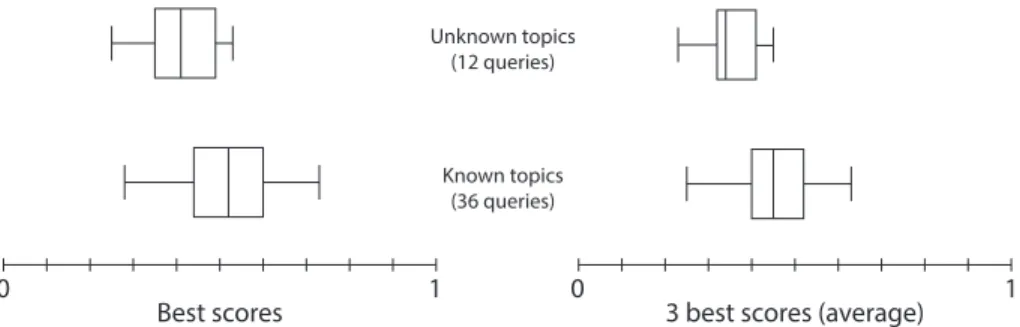
It is also interesting to examine the proximity score distribution for queries with known and unknown topics. Figure 3 shows that the scores for Top 1 and Top 3 (average of 3 scores) are lower when the topic is not present in the database. This is of course expected. However, in some cases, the proximity score for a known topic may be low, while on the opposite, an unknown topic may still reach a relatively high score. For instance, the best score for a query about “Government investment” (in a table we have) is 0.42, while the best score for “GDP per capita” (on which we do not have data) is 0.53. Thus, our current scores, alone, do not suffice to confidently determine whether our database does contain the information requested in a query.
0 1 0 1
Best scores 3 best scores (average)
Unknown topics (12 queries)
Known topics (36 queries)
Fig. 3. Score distribution for known and unknown topics
Thus, while our algorithm works generally well, the best approach appears to be to show the user the highest-rank datasets and let her chose the one(s) that look more promising, similarly to the way in which Web search engines work.
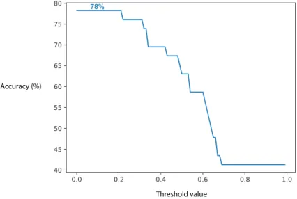
Dimensions To test our identification of data dimensions in queries, we wrote 40 queries on 10 tables (4 queries per table). Each query specifies one value for one dimension of the table. For example, the query “Female population in Russia” would concern the dimension “SEX” with the value “FEMALE”. Furthermore, 6 queries contained a comparison of dimension values, introduced through “than” (e.g., “Countries with more male population than female”). The value of a dimension can be specified (“MALE” or “FEMALE”) or can default to “TOTAL”. For each query, we assess if this specific dimension was given the correct value by the algorithm: we obtained 78% accuracy with no notable differences across query groups. Compared with other accuracy results, these are a bit lower, but they still show relatively good performance.
Another question we study is the utility of a threshold similarity score (recall Section 6). Figure 4 plots the accuracy of dimension understanding from the
Accuracy (%)
Threshold value 78%
Fig. 4. Accuracy of dimension understanding from user queries vs. similarity threshold.
query, against the value of this threshold. The most accurate results are obtained with the lowest threshold, i.e., in general, the best value for the dimension is the one with the highest score, even if this score is quite low. However, it is worth noting that our test queries only used one dimension, e.g., they do not simultaneously constrain the gender and the age of people (mostly because the data we had access to did not provide interesting, meaningful combinations of dimensions). Thus, our observations on the threshold are based on such single-dimension queries. In general, care should be taken not to set the threshold too low, so as not to miss dimension(s) matched with lower similarity.
8
Related work
Chatbots have become ubiquitous tools for human-computer interaction [11]. While some are designed to handle conversations with the user, others are built for specific tasks, e.g., book plane tickets). Our work falls into the second cate-gory. The general framework for this kind of systems is to use the user’s inputs to fill a set of frames (origin city, destination city, departure time...) and once everything is complete, execute the task (book the tickets). Some tools like Di-alogFlow (Google) or Wit.ai (Facebook) offers turnkey solutions for developers to specify the desired frames and let AI models fill them automatically.
To facilitate the task of querying relational databases, several works pro-posed natural-language query interfaces which are given user queries in natural language and translate them into SQL queries, e.g., [15,16]. Prior efforts in fa-cilitating access to high-quality statistical data have focused first, on extracting the data out of HTML pages and HTML or Excel tables [4] and then on develop-ing a specific keyword search algorithm for finddevelop-ing the datasets (and, if possible,
dataset cells) most pertinent for answering a query [5]. A claim extraction tool [6] focused on extracting, from a natural language phrase making some statement about a statistical quantity, the quantity name and possible dimensions.
The need for question answering systems over Linked Data has grown in sync with the popularity of the RDF4 format and the development of its associated query language, i.e. SPARQL5. Several projects have aimed at implementing QA systems over large linked datasets, for instance DBpedia [2]. The RDF Data Cube Vocabulary6 gives the RDF format additional means to deal with multi-dimensional linked data, such as statistics. A lot of research works have been done on the Question Answering on Data Cubes [10,3,9]. Challenges also take place regularly to assess state of the art techniques in this field [17].
We tried to build our system using a different approach compared to these existing works. First, because this high-quality data is specifically available in SDMX, we wanted to stick to this format. Even though a lot of similarities exist between SDMX and Data Cubes, we wanted to take advantage of the SDMX specificities (like the extended metadata) rather than just doing a format translation and using another system. Moreover, these works usually include machine learning methods based on neural networks. In this study, given the relatively simple shape of the questions we expect over the statistical databases, we have not relied upon such methods. Instead, we used a rule-based approach based on the question syntax to classify and understand the question, and relied on linguistic distance to determine the dataset that is closest to the query.
9
Conclusion and future work
Among existing agents and natural language interfaces to databases, the novelty of our work is to be the first to consider the development of a system over SDMX data. Sponsored by major international institutions such as the European Central Bank, Eurostat, the International Monetary Fund, the United Nations and the World Bank, SDMX allows sharing datasets across institutions and facilitates their processing by stakeholders (government at all levels, the press, interested citizens). Large volumes of SDMX data are published and exchanged by these and other institutions. In this study, we only had access to an endpoint (Web service capable of answering structured queries sent by the algorithm) publishing a limited amount of data. Future work could test and consolidate our methods on more data, improve the accuracy of our topic understanding, and implement the conversational capabilities of a chatbot.
Acknowledgments We thank Eric Anvar, Head of Smart Data Practices and Solutions at OECD, Jonathan Challener, Partnerships and Community Manager at OECD, for their suggestions and support. This work was partially funded by the ANR Project ContentCheck (ANR-15-CE23-0025).
4 https://www.w3.org/RDF/ 5
https://www.w3.org/TR/sparql11-query/ 6
References
1. SDMX (Statistical Data and Metadata eXchange). https://sdmx.org/ (2020) 2. Athreya, R., Ngonga Ngomo, A.C., Usbeck, R.: Enhancing community
inter-actions with data-driven chatbots–the DBpedia chatbot. pp. 143–146 (2018). https://doi.org/10.1145/3184558.3186964
3. Atzori, M., Mazzeo, G.M., Zaniolo, C.: Querying rdf data cubes through natural language. In: SEBD (2018)
4. Cao, T.D., Manolescu, I., Tannier, X.: Extracting linked data from statis-tic spreadsheets. In: Int’l. Workshop on Semantic Big Data (2017). https://doi.org/10.1145/3066911.3066914, https://hal.inria.fr/hal-01583975 5. Cao, T.D., Manolescu, I., Tannier, X.: Searching for Truth in a Database of
Statis-tics. In: WebDB. pp. 1–6 (Jun 2018), https://hal.inria.fr/hal-01745768 6. Cao, T.D., Manolescu, I., Tannier, X.: Extracting statistical mentions from textual
claims to provide trusted content. In: NLDB (Jun 2019), https://hal.inria.fr/ hal-02121389
7. Cazalens, S., Lamarre, P., Leblay, J., Manolescu, I., Tannier, X.: A Content Man-agement Perspective on Fact-Checking. In: The Web Conference 2018 - alternate paper tracks ”Journalism, Misinformation and Fact Checking”. pp. 565–574. Lyon, France (Apr 2018), https://hal.archives-ouvertes.fr/hal-01722666
8. Finkel, J.R., Grenager, T., Manning, C.: Incorporating non-local information into information extraction systems by Gibbs sampling. In: ACL. pp. 363–370 (2005), http://nlp.stanford.edu/~manning/papers/gibbscrf3.pdf
9. H¨offner, K., Lehmann, J.: Towards question answering on statistical linked data. In: In’tl Conf. on Semantic Systems (SEM). p. 61–64 (2014)
10. H¨offner, K., Lehmann, J., Usbeck, R.: Cubeqa—question answering on rdf data cubes. In: ISWC (2016). https://doi.org/10.1007/978-3-319-46523-420
11. Jurafsky, D., Martin, J.H.: Speech and Language Processing (3rd ed. draft), Chapter 26 : Dialog Systems and Chatbot. (2019), http://web.stanford.edu/ ~jurafsky/slp3/
12. Manning, C.D., Surdeanu, M., Bauer, J., Finkel, J., Bethard, S.J., McClosky, D.: The Stanford CoreNLP natural language processing toolkit. In: ACL (System Demonstrations). pp. 55–60 (2014), http://www.aclweb.org/anthology/P/P14/ P14-5010
13. Mikolov, T., Chen, K., Corrado, G., Dean, J.: Efficient estimation of word repre-sentations in vector space. In: Proceedings of Workshop at ICLR (2013), https: //arxiv.org/pdf/1301.3781.pdf
14. Miller, G.A.: Wordnet: A lexical database for english. In: Communications of the ACM Vol. 38, No. 11. pp. 39–41 (1995), https://arxiv.org/pdf/1301.3781.pdf 15. Quamar, A., Lei, C., Miller, D., Ozcan, F., Kreulen, J., Moore, R.J., Efthymiou, V.: An ontology-based conversation system for knowledge bases. In: ACM SIGMOD. pp. 361–376 (2020). https://doi.org/10.1145/3318464.3386139
16. Saha, D., Floratou, A., Sankaranarayanan, K., Minhas, U.F., Mittal, A.R., ¨Ozcan, F.: ATHENA: an ontology-driven system for natural language querying over re-lational data stores. Proc. VLDB Endow. 9(12), 1209–1220 (2016), http://www. vldb.org/pvldb/vol9/p1209-saha.pdf
17. Usbeck, R., Gusmita, R., Saleem, M., Ngonga Ngomo, A.C.: 9th challenge on question answering over linked data (qald-9) (11 2018)
18. SOAP Version 1.2. https://www.w3.org/TR/soap12/
19. Web Services Description Language (WSDL) Version 2.0. https://www.w3.org/TR/wsdl/