HAL Id: hal-03006342
https://hal.archives-ouvertes.fr/hal-03006342
Submitted on 15 Nov 2020
HAL is a multi-disciplinary open access
archive for the deposit and dissemination of
sci-entific research documents, whether they are
pub-lished or not. The documents may come from
teaching and research institutions in France or
abroad, or from public or private research centers.
L’archive ouverte pluridisciplinaire HAL, est
destinée au dépôt et à la diffusion de documents
scientifiques de niveau recherche, publiés ou non,
émanant des établissements d’enseignement et de
recherche français ou étrangers, des laboratoires
publics ou privés.
with single-trial response time decomposition
Gabriel Weindel, Royce Anders, F.-Xavier Alario, Boris Burle
To cite this version:
Gabriel Weindel, Royce Anders, F.-Xavier Alario, Boris Burle.
Assessing model-based
infer-ences in decision making with single-trial response time decomposition.
Journal of
Experimen-tal Psychology: General, American Psychological Association, 2021, Advance online publication,
�10.1037/xge0001010�. �hal-03006342�
Assessing model-based inferences in decision making with single-trial
response time decomposition
Gabriel Weindel
Aix Marseille Univ., CNRS, Marseille, France
Royce Anders
Aix Marseille Univ., CNRS, Marseille, France Univ Lumière Lyon 2, Lyon, France
F.-Xavier Alario
Aix Marseille Univ., CNRS, Marseille, France University of Pittsburgh, PA 15213, USA
Boris Burle
Aix Marseille Univ., CNRS, Marseille, France
The latent psychological mechanisms involved in decision-making are often studied with quantitative models based on evidence accumulation processes. The most prolific example is arguably the drift-diffusion model (DDM). This framework has frequently shown good to very good quantitative fits, which has prompted its wide endorsement. However, fit quality alone does not establish the validity of a model’s interpretation. Here, we formally assess the model’s validity with a novel cross-validation approach based on the recording of muscular activities, which directly relate to the standard interpretation of various model parameters. Specifically, we recorded electromyographic activity along with response times (RT s), and used it to decompose every RT into two components: a pre-motor time (PMT ) and motor time (MT ). The latter interval, MT , can be directly linked to motor processes and hence to the non-decision parameter of DDM. In two canonical perceptual decision tasks, we manipulated stimulus strength, speed-accuracy trade-off, and response force, and quantified their effects on PMT, MT , and RT . All three factors consistently affected MT. The DDM parameter for non-decision processes recovered the MT effects in most situations, with the exception of the fastest responses. The extent of the good fits and the scope of the mis-estimations that we observed allow drawing new limits of the interpretability of model parameters.
Introduction
Understanding how decisions are made is an important endeavor at the crossroads of many research programs in cognitive psychology and neuroscience. According to one prevalent theoretical framework, decisions are driven by a cognitive mechanism that sequentially samples goal-relevant information from the environment. Contextual evidence is accumulated in favor of the different alternatives until one of them reaches a threshold that triggers the execution of the
G. Weindel, LPC, UMR 7290 and LNC UMR 7291, Aix-Marseille Univ., CNRS; R. Anders, LPC, UMR 7290 and EMC EA 3082, Univ Lumière Lyon 2; F.-X. Alario, LPC, UMR 7290 , Aix-Marseille Univ., CNRS; B. Burle LNC, UMR 7291, Aix-Marseille Univ., CNRS.
We thank Thibault Gajdos for an early review of the manuscript, and Thierry Has-broucq, Mathieu Servant and Michael Nunez for valuable comments. We thank the four reviewers for their thorough and helpful comments and suggestions on earlier versions of the manuscript. This work, carried out within the Labex BLRI (ANR-11-LABX-0036), the Institut Convergence ILCB (ANR-16-CONV-0002) and NeuroMar-seille (AMX-19-IET-004), has benefited from support from the French government, managed by the French National Agency for Research (ANR) and the Excellence Ini-tiative of Aix-Marseille University (A*MIDEX).
All data and code used in this study are available athttps://osf.io/frhj9/. The last two authors share senior authorship. Correspondence concerning this article should be addressed to Boris Burle, Laboratoire de Neurosciences Cognitives, Case C, Aix-Marseille Université, 3 Place Victor Hugo, 13331 Marseille, cedex 3. E-mail: [email protected]
corresponding response (Ratcliff, Smith, Brown, & McKoon,
2016; Stone, 1960). Typically, this theoretical framework is implemented quantitatively as a continuous diffusion pro-cess. These models are applied empirically to fit response accuracy and latency measures along different alternative-choice tasks and experimental manipulations. Such quan-titative modeling procedures yield data-derived process pa-rameters that are used to infer the cognitive dynamics un-derlying decision-making, which are otherwise not directly observable.
There are multiple variants of these quantitative models, which specify the dynamics of evidence accumulation dif-ferently (e.g., Anders, Alario, & van Maanen,2016;Brown & Heathcote,2008;Heathcote & Love,2012;Palmer, Huk, & Shadlen,2005;Ratcliff,1978;Ratcliff & McKoon,2008;
Tillman, Van Zandt, & Logan,2020;Usher & McClelland,
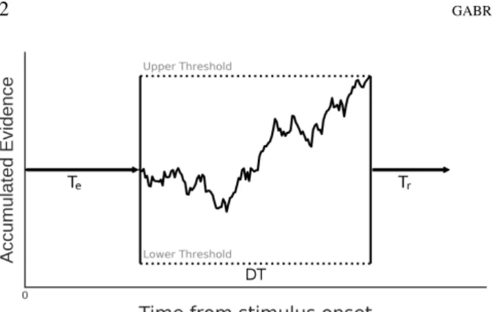
2001, among many others). All of these variants share the hypothesis that each response time (RT ) is the sum of three major terms (Equation1; seeLuce,1986): the time needed for stimulus encoding (Te), the time needed for the
accumu-lated evidence to reach a threshold once accumulation has started (“decision time”: DT ), and the time needed for re-sponse execution (Tr). If the decision-relevant information
Figure 1. Processing account of a single decision in a di ffu-sion model implementing evidence accumulation.
The stochastic path represents the stimulus evidence being accumulated over time through a noisy channel, modeled as a diffusion process with a drift (i.e., rate of accumulation). Accumulation stops once a threshold boundary is reached, and the corresponding alternative is chosen.
encoding reaches the same level of completeness on each trial, Te does not affect the decision-making process of
ev-idence accumulation (DT ). It is also usually assumed that the way the response is executed does not depend on how the decision was reached. In other words, Tr is assumed to
be independent from DT . For these reasons, presumably, the terms Teand Trare most often pooled into a single parameter
Ter(Equation2).
RT = Te+ DT + Tr (1)
Ter= Te+ Tr (2)
In the minimal form of the model, the decision time DT is derived from two parameters: the accumulation rate (i.e., amount of evidence accumulated per time unit) and the decision threshold (i.e., the amount of accumulated evidence needed for a response to be triggered; Figure 1). The best fitting parameters are directly estimated from the measured RT and the corresponding response accuracy.
These models provide a framework to determine the cog-nitive locus of specific experimental observations (e.g., as-sociative vs. categorical priming: Voss, Rothermund, Gast, & Wentura,2013; masked vs. unmasked priming: Gomez, Perea, & Ratcliff, 2013; among many others). They have also been used to assess populations differences. For exam-ple, general slowing associated with aging has been linked to a higher evidence threshold and a longer Ter, rather than
lower evidence accumulation rate (Ratcliff, Thapar, & McK-oon,2001). The same rationale for group analyses is increas-ingly used in psychopathology research to characterize infor-mation processing alterations in a variety of pathologies such as anxiety (linked to a higher rate of accumulation for threat-ening stimuli:White, Ratcliff, Vasey, & McKoon,2010),
de-pression (Lawlor et al.,2019;Pe, Vandekerckhove, & Kup-pens,2013), schizophrenia (Moustafa et al.,2015), Parkin-son’s disease (Herz, Bogacz, & Brown,2016), language im-pairments (Anders, Riès, van Maanen, & Alario,2017), and so on (seeRatcliff et al.,2016, for a review).
This brief overview illustrates the different cognitive ap-plications for which the modelling framework has notably intervened. It reflects the widespread endorsement of the framework by the scientific community as an instrumental cognitive model for characterizing the latent processing dy-namics of decision-making. As researchers are faced with the challenge that cognitive dynamics (in decision-making, or elsewhere) are not directly observable, the role of these process models is to provide inferences, or linking functions from currently observable data (e.g. RTs, accuracy) which is an ambitious step beyond the classical statistic models (e.g. regression, mixed models, etc.) that are only descriptive at various depths of analysis (Anders, Oravecz, & Alario,2018;
Anders, Van Maanen, & Alario,2019). Such cognitive pro-cess models are a crucial research development to the quan-titative rigour of our domain. Their viability, however, de-pends not only on their goodness of fit to data, but also on the interpretative (cognitive) validity of the estimated param-eters. This indispensable, latter condition depends on a num-ber of key assumptions being met, as follows.
First, in using this framework, one has to assume that the postulated model indeed reflects the process generating the behavior. This assumption is often considered to be sup-ported by the quality of the data fit diagnostics (e.g. by RT quantile residualsRatcliff & McKoon,2008), which is gen-erally very satisfactory in most published applications.
However, it has often been reported that a given behav-ioral data-set can be fitted equally well with different models, that differ substantially in their architectures (e.g. Donkin, Brown, Heathcote, & Wagenmakers,2011;Servant, White, Montagnini, & Burle,2016). Therefore, although a good fit is a necessary criteria, it might not be sufficient to single out a particular model (Roberts & Pashler,2000). In addition, while generally robust, model fitting procedures are complex operations that may suffer from problems such as parameter trade-off, sensitivity to trials generated from another genera-tive model (e.g. guessed responses), or other biases that can impact the estimated parameters, and hence notably affect the validity of the inferences made upon them (Ratcliff & Childers,2015).
Secondly, one has to assume that the manipulations that modulate the estimated parameters can indeed be attributed to modulations of the presumed cognitive process. The ma-jor diagnostic to ascertain this mapping is known as the “Se-lective Influence Test” (Heathcote, Brown, & Wagenmakers,
2015). This approach probes whether a given experimental manipulation, presumed to selectively-affect a given psycho-logical process, only affects the corresponding parameter of
the model. For example, manipulations of stimulus informa-tion quality are expected to selectively affect the accumu-lation rate (Ratcliff & McKoon,2008; Voss, Rothermund, & Voss, 2004), and manipulations of response execution are expected to selectively affect the Terparameter (Gomez,
Ratcliff, & Childers,2015; Voss et al.,2004). Perhaps the paradigmatic example of selective influence has been the manipulation of the participants’ response caution, which is implemented by instructions that either emphasize speed or accuracy, in what is known as the speed-accuracy trade-off (“SAT”). This manipulation has originally been shown to se-lectively affect the threshold parameter, which governs the amount of evidence accumulated by participants before they trigger a response (e.g.Ratcliff & McKoon,2008).
Unfortunately, selective influence has proven to be an elu-sive goal. For example, Voss et al.(2004) showed that the SAT manipulation could also affect the non-decision time pa-rameter (see alsoPalmer et al.,2005;Ratcliff,2006). Then
Rae, Heathcote, Donkin, Averell, and Brown (2014) ob-served an effect of SAT manipulation on drift rate, although
Starns and Ratcliff(2014) did not find evidence for this effect in multiple data sets. In a multi-lab collaborative project, Du-tilh et al.(2019) asked a number of expert decision-making modelers to map an anonymous experimental manipulation from de-labeled datasets to the appropriate model parame-ter. Most modelers mapped the effect to the boundary pa-rameter, but also to the drift rate or the non-decision time. The experimental manipulation in the data set was in fact the SAT. In a different dataset, the unknown manipulation was stimulus quality. Some modelers mapped this manipulation to the boundary parameter, in addition to the drift. Dutilh et al. (2019) attributed these uncertainties to an excessive number of degrees of freedom available to the modelers. Al-though the authors noted general agreement across modeling approaches in the main parameters at stake, this study illus-trates the challenges modelers face in consistently attributing manipulation effects to model parameters. It should be high-lighted that the discrepancy might not necessarily be charged onto the modelers and on matters of model fitting (seeSmith & Lilburn,2020, for a recent development). While the selec-tivity of the experimental manipulations is assumed, it is by no means mandated.
In short, two crucial assumptions must be scrutinized: the link between the postulated model and the process of interest, and the link between the experimental effects on the param-eters and the modulation of the processes of interest. One way to address the aforementioned issues associated with those assumptions is to implement additional modeling con-straints through advanced validation measures. These may be derived from data sources co-registered during the exper-iment, ideally data that could provide a direct correlate or measure of the candidate process. For example, various re-searchers have linked decision-making variables with
neuro-physiological activity measured in multiple species, such as rodents (e.g.Brunton, Botvinick, & Brody,2013), monkeys (e.g.Purcell et al.,2010;Ratcliff, Cherian, & Segraves,2003;
Roitman & Shadlen,2002), and humans (e.g.Donner, Siegel, Fries, & Engel,2009;O’Connell, Dockree, & Kelly,2012;
Philiastides, Ratcliff, & Sajda,2006). As a result, these ap-proaches have provided essential additional information on latent decision-making dynamics not previously available.
While this approach, to incorporate other physiological measures that also indicate cognitive processing, is undoubt-edly fruitful, it is still suffering from several unresolved chal-lenges that limit its capacity to validate the current modeling framework. Firstly, one major issue is that it is still not clear how to appropriately link physiological activity metrics to psychological processes (Schall,2004,2019; Teller,1984). For example, neuronal discharge frequency increases as a ramping function during decision-making, in a manner very similar to the postulated model dynamic (Figure1). But such ramping activity has been observed in several brain areas (Purcell et al.,2010;Roitman & Shadlen,2002; overview in
de Lafuente & Romo,2006), making it difficult to unambigu-ously map multiple accumulations into a single cognitive ac-cumulator, or parameter therein. Another limitation comes from the rather low signal-to-noise ratio available in neuro-physiological recordings, which results in findings based on averaged data (e.g., peri-stimulus time histograms, averaged event related potentials, etc.) The information contained in these signals averaged across trials is overly distorted (e.g.
Burle, Roger, Vidal, & Hasbroucq,2008; Callaway, Halli-day, Naylor, & Thouvenin,1984;Dubarry et al.,2017; La-timer, Yates, Meister, Huk, & Pillow,2015), compared to the distributions afforded by single trial analyses (the resolution at which the RT model in question operates on).
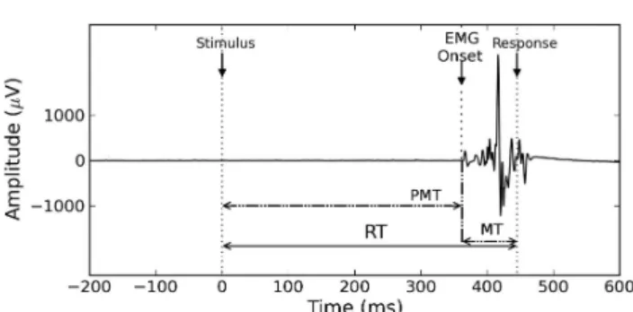
Here, we propose an alternative neurophysiological mea-sure that circumvents some of these limitations, and demon-strate how it can be used to address the previously-discussed issues of parameter attribution and inferential validity of the modeling. This neurophysiological measure is the elec-tromyographic (EMG) activity of the effector muscles that perform the responses. In contrast to lateralized readiness potentials computed from electro-encephalogram (Osman et al.,2000;Rinkenauer, Osman, Ulrich, Muller-Gethmann, & Mattes,2004), the high signal-to-noise ratio of EMG allows for a reliable decomposition of the RT of every single trial into two subcomponents: the time from stimulus onset to EMG onset (“pre-motor time”, PMT ), and the time from EMG onset to the behavioral response (“motor time”, MT ;
Botwinick & Thompson,1966;Burle, Possamaï, Vidal, Bon-net, & Hasbroucq, 2002; Figure 2). While the PMT cer-tainly contains many processes, linking the recorded MT with a psychological process is more straightforward. As
Luce (1986, p.97) states, “the time from that event [EMG onset] to the response is a proportion of the entire motor time
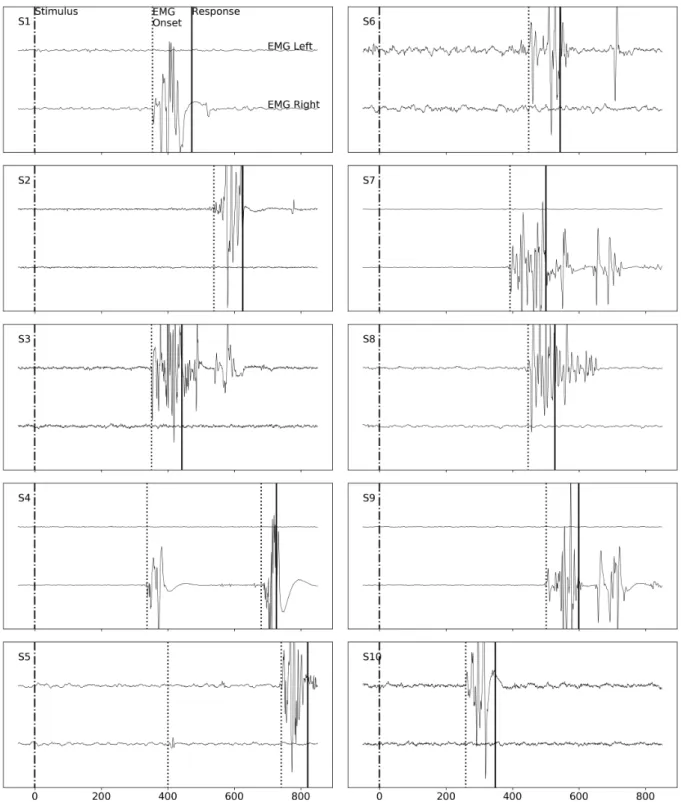
Figure 2. Single-trial RT decomposition using EMG The Pre-Motor Time PMT is the time between stimulus and EMG onsets; the Motor Time MT is the time between the EMG onset and the mechanical response. See FigureA1for additional examples of EMG recordings.
and that, in turn, is a proportion of the residual R [in our no-tation, Ter]”. In other words, the time postulated in the model
to execute the response (Trin Equation2) should be strongly
related to the recorded MT .
The relationship between MT and Tr might be
compli-cated by the fact that typical fitting procedures provide val-ues for Ter, not Tr. However, as proposed byLuce(1986, p.
118) :
The assumption is that if R’ [here, MT ] exhibits a dependence upon signal intensity [or other fac-tors], then the chances are that R [here, Ter] will be
affected also, which it will be unless the effects on R’ and R - R’ are equal and opposite - an unlikely possibility.
Following this rationale, if the covariance across trials be-tween MT and Ter turned out to be weak or non-existent,
then one would have to conclude that the measured MT is not contained in the estimated Ter. Consequently, if it is hence
the case that Terdoes not incorporate response execution
pro-cesses, this would severely put into question the current cog-nitive interpretative validity of this parameter, and hence of the other parameters too.
Previous research has already shown that the measured MTis not a mere constant value added to the PMT . Its vari-ability contributes to the overall performance one (i.e of the RTs). Furthermore, MT s have been found to be modulated by certain experimental manipulations. Early on, Grayson
(1983) suggested that stimulus intensity affects the estimated MT in a simple reaction task, andServant et al. (2016) re-ports a recent confirmation. It has also been shown that MT0s are shortened if advance information is provided about the timing (Tandonnet, Burle, Vidal, & Hasbroucq,2003,2006) or about the nature (Possamaï, Burle, Osman, & Hasbroucq,
2002) of the forthcoming stimulus or response.
Even if the functional interpretation of such perceptual
and decisional effects on late motor processes is still under discussion, the observations suggest that certain effects de-tected in the RT s, even among those assumed to be “cogni-tive/ decisional”, could be driven in part by modulations in motor processes. Inasmuch as motor time can be mapped to the parameter capturing response time execution Tr (see
above), this conclusion contradicts one of the assumptions often made about non-decision processes, which was sum-marized byTurner, Van Maanen, and Forstmann (2015, p. 316) : “[. . . ] the non-decision time parameter captures ef-fects that are not cognitively interesting [. . . ]”. The alterna-tive possibility that non-decision time is cognialterna-tively relevant has important implications for models of decision making.
The Present Study
The present study is based on two experiments, each in-volving a standard perceptual decision task. Our main hy-pothesis in this study is that decomposing RT s through EMG techniques into PMT and MT will help 1) better establish the locus of certain experimental manipulations, 2) test some central assumptions of the modeling framework regarding the postulated cognitive processes, and 3) assess to what ex-tent EMG-based and model-based decompositions of RT s provide (di)similar information about the non-decision time parameter.
Visual contrast was manipulated to adjust task difficulty, and verbal instructions emphasizing speed or accuracy were used to implement an SAT setting. Across the two exper-iments, we also manipulated the force required for the re-sponse to be produced. We recorded the EMG activation and the latency of every manual response, hence deriving single trial distributions not only for RT , but also for PMT and MT , and assessed the impact of the experimental factors on each of these variables. Based on previous studies (Spieser, Ser-vant, Hasbroucq, & Burle,2017;Steinemann, O’Connell, & Kelly,2018, see alsoOsman et al.,2000;Rinkenauer et al.,
2004, who suggested the existence of a SAT effect on motor
processes using LRP), we expected that the measured MT would be affected by SAT, and possibly by stimulus strength (Grayson,1983;Servant et al.,2016). In addition, by having a reliable EMG measure for every single trial, we were able to assess the stochastic dependency between PMT and MT . In other words, this provides a test for the subsidiary assump-tion of independence between decision and non-decision pro-cesses, a test that is not possible in most regular parameter estimation procedures.
Following this empirical exploration, we estimated the pa-rameters of the Drift Diffusion Model (DDM;Ratcliff,1978;
Ratcliff & McKoon,2008) from the data using a hierarchi-cal Bayesian fitting method (Wiecki, Sofer, & Frank,2013, HDDM package). First, we applied a model selection pro-cedure to find the best fitting model. Secondly, we evaluated the correlation between the estimated Terparameter and the
measured MT , across participants. Finally, we fitted a joint DDM that takes the MT as a by-trial regressor, to assess the link between the Terparameter and the measured MT .
Experiment 1 Methods
Participants. Sixteen participants (8 men and 8 women, mean age= 23.5, 2 left-handed) that were students at Aix-Marseille University, were recruited for this study. They were compensated at a rate of 15e per hour. All participants reported having normal or corrected vision, and no neurolog-ical disorders. The experiment was approved by the ethneurolog-ical experimental committee of Aix-Marseille University, and by the “Comité de Protection des Personnes Sud Méditerrannée 1” (Approval n° 1041). Participants gave their informed writ-ten consent, according to the declaration of Helsinki.
Apparatus. Participants performed the experiment in a dark and sound-shielded Faraday cage. They were seated in a comfortable chair in front of a 15 inch CRT monitor placed 100 cm away, that had a refresh rate of 75 Hz. Responses were given by pressing either a left or a right button with the corresponding thumb. Buttons were fixed on the top of two cylinders (3 cm in diameter, 7.5 cm in height) separated by a distance of 20 cm. They were mounted on force sen-sors allowing to continuously measure the force produced (A/D rate 2048 Hz), and to set the force threshold needed for the response to be recorded. In Experiment 1, this response threshold was set to 6N (600g). Response signals (threshold crossing) were transmitted to the parallel port of the record-ing computer with high temporal accuracy (< 1ms). At but-ton press, participants heard a 3ms sound feedback at 1000 Hz (resembling a small click). The forearms and hypothenar muscles of the participants rested comfortably on the table in order to minimize tonic muscular activity compromising the detection of voluntary EMG bursts. We measured the EMG activation of the flexor pollicis brevis of both hands with two electrodes placed 2 cm apart on the thenar emi-nences. This activity was recorded using a BioSemi Active II system (BioSemi Instrumentation, Amsterdam, the Nether-lands). The sampling rate was 2048 Hz.
Stimuli. Stimuli presentation was controlled by the soft-ware PsychoPy (Peirce,2007). Each stimulus was composed of two Gabor patches, presented to the left and the right of a fixation cross. The Gabor patches had a spatial frequency of 1.2 cycles/visual angle degree and had a size of 2.5 visual an-gle degrees each. The standard Gabor patch contrast was set to 0.5, on a scale between 1 (maximum contrast) and 0 (uni-form gray). Five levels of stimulus contrast were used (0.01, 0.025, 0.07, 0.15, 0.30). These contrast values were added to the target Gabor patch and subtracted from the distractor Gabor patch. These contrast levels were decided based on performance from a pilot study where they were found to
yield a full range of performance quality: from near perfect to almost chance level accuracy. The task of the participants was to press the button (left or right) ipsilateral to the patch with the highest contrast.
Procedure. All participants performed one single ses-sion with 24 blocks of 100 trials each. Sesses-sion duration was approximately 1h30, including a training session of 15 min-utes and self-paced breaks between each block. During the training session, participants were instructed that “Speed” in-structions required a mean RT near 400 ms and that “Accu-racy” instructions required a minimal response accuracy near 90% while maintaining RT s below 800 ms. Participants were also informed to keep their gaze on the central fixation cross during the blocks.
The beginning of each speed or accuracy block was pre-ceded by the corresponding visual instruction (the French word “Vitesse” or “Précision” for Speed and Accuracy, re-spectively). The end of each block was followed by the pre-sentation of the recorded mean RT and response accuracy performance of the block, along with oral feedbacks from the experimenter in those cases were the participant did not sat-isfy the condition goals. The training session included 40 tri-als without performance instructions followed by 2 blocks of 10 trials in the Speed condition, followed by 2 blocks in the Accuracy condition, and ended with 4 blocks of 10 trials with alternating instructions. For the experimental session, speed instructions alternated every three consecutive blocks. The order of the instructions was counterbalanced across partici-pants. The contrast conditions of the stimuli were fully ran-domized across the 5 levels within each block. No response deadline was applied, the stimulus disappeared when partic-ipant produced a button press, the response-stimulus interval was fixed to 1000ms.
EMG processing. The EMG recordings were read in Python using the MNE module (Gramfort et al.,2013), and filtered using a Butterworth 3rd order high pass filter at 10Hz from the scipy Python module (Oliphant,2007). The by-trial EMG signal was then processed in a window between 150 ms before, and 1500 ms after stimulus onset. A variance-based method was used to detect whether EMG activation was sig-nificantly present in either hand’s channel. The precise on-set was then identified with an algorithm based on the “In-tegrated Profile” of the EMG burst. This method takes the cumulative sum of the rectified EMG signal on each epoch and subtracts it from the straight line joining the first and the last data-points (corresponding to the cumulative sum of an uniform distribution). The onset of the EMG burst cor-responds to the minimum of this difference (seeLiu & Liu,
2016;Santello & Mcdonagh,1998for more details1). The EMG onsets determined by the algorithm were examined by
1A software implementing this two steps procedure will soon be
released with an open-source license, and is already accessible upon request.
the experimenter who could perform manual corrections as needed (18.3% of the trials). For this processing stage, the experimenter was unaware of the trial type he was exam-ining, to avoid any correction bias. Every muscular event (rapid change in the signal followed by a return to the base-line) in the trial was marked, thus quantifying how many times the muscle was triggered, even when the identified ac-tivation did not lead to an overt response (see FigureA1for examples of recorded EMG activity).
Motor time (MT ) was defined as the time between the on-set of the last EMG activation preceding the responding hand button press. Pre-motor time (PMT ) was defined as the time between stimulus onset and this last EMG onset. In this way, any intervening EMG activations were discarded. For the purpose of this study, we treated the trials with multiple ac-tivities (25.90% of the total number of trials, see for example participants S4 and S5 EMG plot in FigureA1) as trials with only the last EMG activation. Notice that if only RT was measured these trials would not have had any special status. It has not escaped our attention that these trials can repre-sent a challenge for evidence accumulation models (Servant, White, Montagnini, & Burle,2015;Servant et al.,2016), and that they will have to be investigated more thoroughly in fu-ture research.
Statistical procedure.
Bayesian Statistics. Apart from a few exceptions (see below), the analyses were performed within the Bayesian framework. Bayesian methods aim to estimate an unknown parameter (or set of parameters) and the uncertainty around it. More explicitly, Bayesian methods implement Bayes’ rule to generate a posterior distribution for each parameter based on a combination of prior information and the likelihood of the data given the parameters. This posterior distribution can then be naturally interpreted as the probability of any given parameter value given the data, the priors and the tested model. In our study, we summarize the posterior distribution using the mean, standard deviation and the 95% Bayesian credible interval (CrI). Our criterion to assess the presence of an effect was that the null value lied outside the CrI. While this method does not quantify the evidence in favor of the null hypothesis, it does provide an estimation of the effect size and its uncertainty. All the priors used in the manuscript are detailed in AppendixB.
Bayesian Mixed Models. To test our hypotheses on the behavioral and EMG variables we used linear mixed models (LMMs). These models estimate fixed effects (e.g. the effect of SAT on RT ) while accounting for random effects ((e.g. the inter-individual differences in the effect of SAT on RT), mak-ing them particularly useful in repeated measure design such as the one used in this study. Estimating inter-individual dif-ferences as random effects shares the information gathered from each participant while providing separate (but not inde-pendent) estimates for each one of them. Given our analysis
approach, we derived one generic LMM fitted independently for all chronometric dependent variables: RT , PMT and MT . In these LMMs, the log transformation of the chronometric variables on the ith trial for the jth participant (yi j) was
as-sumed to be drawn from a normal distribution with mean µj
and residual standard deviation σr:
yji∼ N (µj, σr) (3)
Where ∼ stands for “distributed as”. The mean of each par-ticipant µjis then defined by an intercept (αj) and slope
co-efficient (βj) for each experimental factor and their
interac-tions.
µj= αj+ β1 jS AT+ β2 jCont. + β3 jCorr.+
β4 jRS+ β12 jS AT × Cont. + β13 jS AT × Corr.+
β23 jCont. × Corr. + β123 jS AT × Cont. × Corr.
(4)
where Cont. stands for “Contrast”, Corr. stands for “Cor-rectness”, and RS stands for “Response side”2. The individ-ual intercepts (αj) and slopes of each predictor x (βx j) are
modelled as drawn from a normal distribution :
αj∼ N (µα, σα) (5)
βx j ∼ N (µβx, σβx) (6)
Where µαand µβx are the population estimated intercept and
slope while σαand σβx the estimated population variance of
the intercept and the slope (i.e. the random effect). In order to test our hypothesis, we report for each LMM the posterior distribution of the population-estimated intercept and regres-sion coefficients.
In Equation4, correctness of the response was included as a predictor because the relationship between the distri-butions of RT on correct and incorrect trials is known to change under speed pressure (Grice & Spiker,1979), and be-cause MT has been previously-reported to be affected by this factor (e.g.Allain, Carbonnell, Burle, Hasbroucq, & Vidal,
2004; Rochet, Spieser, Casini, Hasbroucq, & Burle,2014;
´Smigasiewicz, Ambrosi, Blaye, & Burle,2020). Response side was included as an additive predictor because left and right RT s often differ. Two remarks are in order concerning this last point. First, we did not expect any interaction with the other predictors. Second, motoneurons synchronization has been shown to depend on handedness (Schmied, Vedel, & Pagni,1994). As a consequence, we can expect Response side to affect MT and the effect to be, at least substantially, of motor origin.
We also tested the effects of these factors on the proportion of correct responses using a generalized linear mixed model assuming that each response (correct or incorrect) was drawn from a Bernoulli distribution whose parameter depends on
2The common R syntax for these LMMs would be : y ∼ SAT *
the same predictors as the LMM (except the correctness fac-tor and its interactions).
For each LMM and generalized LMM, 6 Markov Chain Monte Carlo (MCMC) sampling processes were run in par-allel, each composed of 2000 iterations among which the first 1000 samples were discarded as warm-up samples. We as-sessed convergence of the MCMC chains both by computing the potential scale reduction factor ( ˆR, see Gelman & Ru-bin,1992) and by means of visual inspection of the MCMC chains. We also visually checked the assumptions of the linear regression by inspecting the normality of the residu-als through QQ-plots and assessment of homeoscedasticity. The LMM and generalized LMM were fitted with a custom Stan code, available in the online repository, inspired from the code provided byNicenboim, Vasishth, Engelmann, and Suckow(2018) and using the pystan package (Stan Devel-opment Team,n.d.). Summary statistics and plots of the pa-rameters were created with the arviz python package (ver-sion 0.4.1,Kumar, Carroll, Hartikainen, & Martin,2019).
We also performed a frequentist replication of each G/LMM using the lme4 R package as a means to check for prior sensitivity. Any discrepancy with the main (Bayesian) analysis is reported in the Results.
Factor Coding and LMM parameter interpretation. For all LMMs, sum-contrasts were used for SAT (-0.5 for speed and 0.5 for accuracy) and for response side (-0.5 for right responses and 0.5 for left responses). Treatment-contrast was used for correctness (0 for correct and 1 for incorrect responses). The stimulus strength factor was cen-tered on its middle value and transformed such that -.5 rep-resented the lowest possible contrast and .5 the highest pos-sible contrast. These coding features were chosen to ease the interpretation of the resulting coefficients. When the binary predictor is sum-contrasted (-0.5 and 0.5), the estimated β value can be read as the difference between both conditions. When the binary predictor is treatment-contrasted (0 and 1), the estimated β can be read as the difference to add to the intercept (predictor at 0) to obtain the mean of the condition where the predictor is at value 1. Hence, in our analysis, the intercept can be read as the predicted time for the reference condition where the response is correct, and at an intermedi-ate value for the predictor SAT. The main effects and interac-tions can be read according to the coding scheme used, e.g. the correctness slope represents the benefit or cost of an error when contrast is at mid-level. The contrast slope represents the benefit or cost of a higher contrast when the response is correct. The interaction between contrast and correctness represents how the correctness/contrast effect changes when contrast is higher than mid-level/an error was made.
RT , PMT and MT specific adjustments. By-trial RT , PMT and MT were log transformed prior to the analysis be-cause these variables have heavily skewed distributions that would violate the normality assumption of residuals of the
LMM. To ease the interpretation of the estimated LMM pa-rameters, we back-transformed the intercepts by taking their exponential, and each slope by subtracting the exponential of the intercept from the exponential of the sum of the inter-cept and slope. We applied this back-transformation at each iteration of the MCMC procedure, hence computing the un-certainty around the parameter values on their natural scale.
Fast guess detection. Before applying any analysis we performed the Exponentially Weighted Moving Average (EWMA) filter developed by Vandekerckhove and Tuer-linckx(2007). This method iteratively computes a weighted accuracy measure (amount of correct responses relative to errors) on the sorted RT distribution, from the fastest to the longest RT . Participants are considered as being in a fast guess state until the weighted accuracy is higher than a de-fined threshold. The RT at which this change of state oc-curs is identified, and all trials faster than this RT are cen-sored. The user defined parameters in this method are the initial starting point of the weighted accuracy, the accuracy threshold for defining non-guess trials, and the amount of preceding trials (weight) retained in the accuracy computa-tion. The starting point was defined at 0.50 based on the assumption that a guessing strategy yields a 50% chance of correct response. The threshold was fixed at 0.60 based on a reasonable assumption that participants were not guessing when accuracy was superior to 0.60. The weight was heuris-tically fixed at 0.02 (bounded from 0 to 1, with 0 being all preceding trials used), after visual inspection of the rejec-tion plots with different weights. This method was applied for each participant’s RT distribution separately in the speed and accuracy conditions, as fast-guesses can have different latencies across both conditions. The figures illustrating these rejection procedures can be found in the online reposi-tory. We thank Michael Nunez for kindly providing the code used for this method (https://github.com/mdnunez/ bayesutils/blob/master/wienerutils.py).
Results
Two of the sixteen participants were excluded due to high tonic activity in the electromyogram, which otherwise would have made the detection of their EMG onsets too unreliable. This rejection was decided before performing any analyses. Due to technical constraints on the methods for detecting EMG onsets, we applied an upper limit of 1500 ms to the RTs, resulting in the loss of 0.50% of the trials. Trials with low signal-to-noise ratio, and trials with high spontaneous tonic activity, making appropriate EMG onset detection dif-ficult, were also removed. In total, these acceptability con-ditions led to the exclusion of 4.08% trials for all analyses. Additionally, the EWMA method removed 5.80% trials of the data.
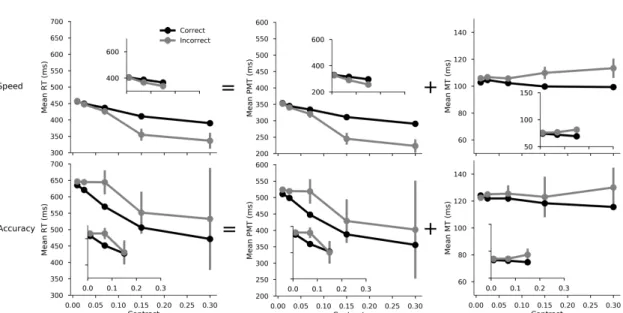
The descriptive statistics discussed for the chronometric variables are summarized in Figure3. The parameters of the
Bayesian LMM are represented on the same scale (in mil-liseconds) in Table1and in Figure4. Additional analyses of response accuracy are provided in AppendixC.
RT and PMT. PMTs and RT s become shorter as con-trast increases and when speed is stressed. Although the credible intervals contained the null value, we observe a weak positive main effect of correctness. However, an in-teraction with SAT instructions showed that when speed is emphasized, errors are faster, and when accuracy is empha-sized, errors are slower. A strong three-way interaction fur-thermore specified that this correctness effect according to SAT conditions is even stronger for easier contrasts. Overall, the results for PMT s and RT s mirrored each other except for one difference: response side (laterality) had a significant effect on the RTs but not on the PMTs (not shown in Figure
3)3.
MT. Replicating previous results, MT s were also faster under speed emphasis. However, contrary to RT and PMT , the effect of correctness was in the same direction in both SAT conditions (slower MT s during errors). MTs were faster when participants responded with their right hand, which explains that the previous laterality effect observed on RTs (but not on PMT s) was due to MT differences. Finally, there was a small but consistent effect of contrast on MT. This effect interacted significantly with response correctness indicating that the lengthening of response execution for er-rors (see Allain et al.,2004; ´Smigasiewicz et al.,2020, for interpretation) was larger in the easier contrast conditions. No additional interactions were observed (see Table1).
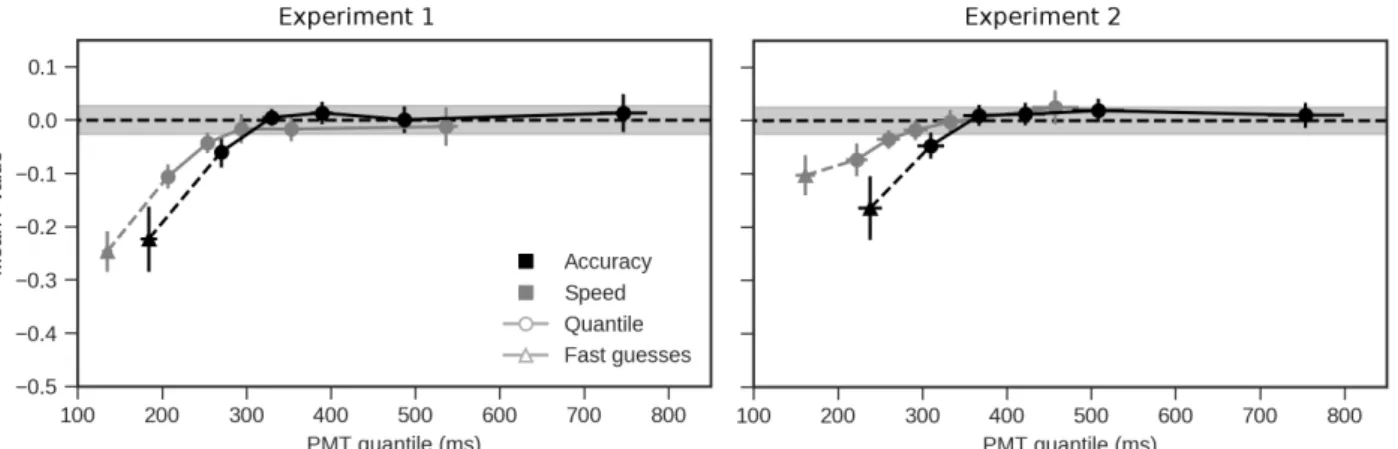
Correlations between PMT and MT. In most imple-mentations of the evidence accumulation framework, the de-cision and non-dede-cision stages are assumed to be indepen-dent from one another. We tested this assumption by exam-ining, for each participant, the Spearman correlation between by-trial PMT s and MT s, in the speed and the accuracy con-ditions separately. It is important to note that certain trial fea-tures may bias the correlation estimates. For example, fast-guess trials defined on the basis of their RT value could bias the computed correlation coefficients towards negative val-ues. Indeed, as the total RT is the sum of PMT and MT , fast RTs most likely result from both fast MT and PMT . Trim-ming lower RT values would remove trials in which PMT and MT likely show a positive co-variation, thus biasing the correlation estimates towards negative values. Additionally, as suggested by Stone(1960), trials with long PMT might be subject to a trade-off between PMT and MT based on an implicit deadline (a process that is not implemented in the DDM), hence generating a negative correlation.
To address these concerns, the correlation between these RT subcomponents was assessed separately for trials iden-tified as fast-guesses and, the remaining trials, for which the correlation was computed across five different quan-tiles (namely, .1, .3, .5, .7, and .9). With respect to fast
guesses, these were identified as before, with the exponen-tially weighted moving average (Vandekerckhove & Tuer-linckx,2007) now based on the sorted distribution of PMT rather than the distribution of RT 4. There was an average of 79.14 fast-guess trials per participant and SAT condition (range: 17-249). There was an average of 1065.93 remaining trials per participant and SAT condition (range: 786-1165), to be divided in 5 quantiles.
For the trials identified as fast guesses, we computed Spearman correlations between PMT and MT within each participant and SAT condition, and submitted these values to an LMM with SAT emphasis as a predictor5. The Accuracy condition was coded as 0 and Speed as 1, thus allowing us to interpret the intercept of the LMM as the mean correlation value when accuracy is emphasized and the slope (effect) as the change in this mean correlation when speed is empha-sized. Fast guesses presented a negative mean correlation in the accuracy condition, as shown by the intercept of the LMM (m= -0.22, 2.5% = -0.33, 97.5% = 0.10). The slope of the LMM (in other words, the change in this mean cor-relation when speed is emphasized) did not suggest that the correlation differed between conditions (m = -0.03, 2.5% = -0.15, 97.5%= 0.09) (see Figure5).
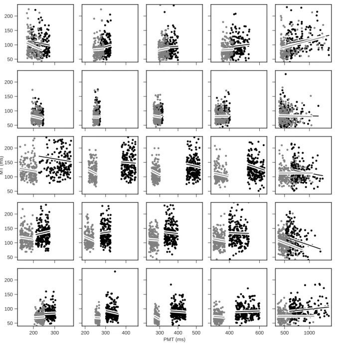
For the correlation analysis along quantiles, the likelihood of the mean correlation coefficient at each quantile was as-sessed with a Monte-Carlo procedure. We computed the Spearman correlation between draws from two random vari-ables following a normal distribution (with mean= 0 and SD = 1) for 14 simulated participants divided into two condi-tions, and 5 bins of data with the same amount of trials as the real data; this procedure was repeated 1,000 times. This non-parametric analysis was motivated by the fact that we did not have a specific hypothesis (e.g. a linear trend) for the effect of the quantiles on the mean correlation value. The first quantile in the speed condition, was outside the range of expected values for the normal variables (Figure5). Like-wise, the first quantile in the accuracy condition was also outside the expected range, even if less negative than in the speed condition. The other correlation values do not differ from random levels. To illustrate the relationship between PMT and MT at the participant level, in Appendix Dwe provide the scatter plots for the first 5 participants across the 5 quantiles.
3A frequentist replication of these tests provided the same
re-sults, except it included an additional significant interaction : be-tween contrast and correctness for PMT (log(β)= −0.07, t = 2.97)
4Both applications of the method revealed a strong but not
per-fect correlation on the amount of censored trials (r(28) = 0.76, p< .001).
5Note that, given low number of points (N= 14), this LMM only
R T PMT MT Predictor Coe ff . SE 2.5% 97.5% Coe ff . SE 2.5 97.5% Coe ff . SE 2.5% 97.5% Intercept 469 12 446 494 354 8 338 370 105 6 93 118 SA T 135 19 101 173 118 17 85 150 15 3 9 22 Contrast -94 10 -114 -74 -81 9 -99 -62 -6 1 -9 -3 Correctness 11 6 0 22 0 6 -11 12 6 1 4 8 Resp. Side 18 6 6 31 0 8 -16 17 17 4 10 24 SA T × Contrast -65 9 -82 -47 -62 8 -78 -44 -1 1 -3 1 SA T × Correctness 71 12 48 96 75 14 49 105 -1 1 -4 2 Contrast × Correctness 26 15 -3 55 3 16 -28 35 13 3 8 18 SA T × Contr . × Corr . 153 32 90 216 164 33 95 228 1 3 -5 7 T able 1 Results of the LMMs in Experiment 1 for eac h latency measur e. Coe ff . indicates estimated coe ffi cients of the LMM fitted on the lo g scale and bac k-tr ansformed to the millisecond-scale . SE indicates the standar d err or for the Coe ff . 2.5 and 97.5% indicate the lower and upper CrI ar ound the Coe ff . F or further details, see the Statistical Pr ocedur e section.
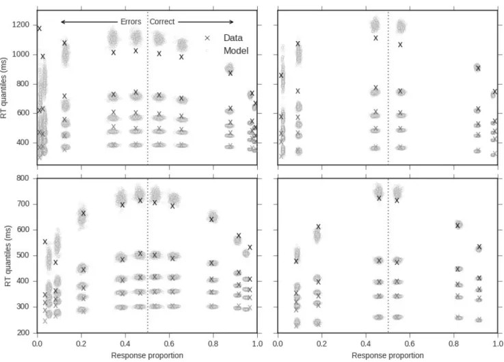
Figure 3. Observed results in Experiment 1, effect of stimulus strength level (contrast) on the mean RT (left column), PMT (center column) and MT (right column). This plot illustrates the interaction between contrast (x-axis), SAT conditions (top vs. bottom rows), and correctness of the response (black - correct vs. grey - incorrect). Bars around the mean represent 95% confidence intervals corrected for within-subject design using the method developed inCousineau (2005). To assess replication, the small insets provide the results obtained in Experiment 2 for a subset of the contrast levels (0.01, 0.07, 0.15). Note: these figures analyze the means in millisecond units, while the LMM analysis presented in Table1model the means in log-transformed units.
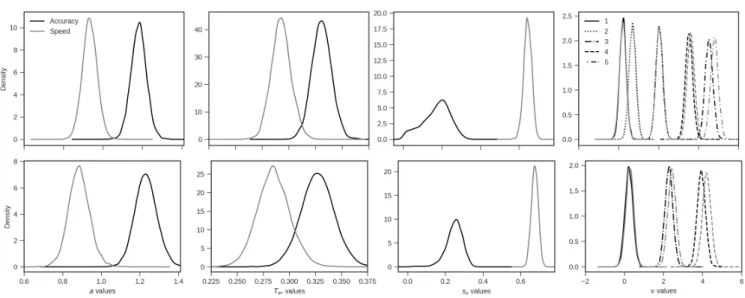
Figure 4. Posterior distributions for the regression coefficients from the LMM model fitted on the RT, PMT, and MT of Experiment 1 (black) and Experiment 2 (grey). The segments around the estimates represent 95% CrIs. As the coefficients for MT are of smaller magnitude, we provide a zoomed inset on the far right of the Figure to ease their visualisation.
Discussion
With respect to the RT s, the different manipulated factors led to clear results that were congruent with previous works discussed in the Introduction. As theories for the potential effects on PMT and MT are less developed, these results will be discussed in more detail in this section.
Firstly, consistent with previous studies, the SAT manip-ulation significantly affected RT and response accuracy (the
latter is reported in AppendixC). In agreement with a deci-sional locus of SAT, this factor also had a large impact on pre-motor time (PMT ). However, the effect of SAT was not restricted to PMT , as this factor also affected MT. This lat-ter observation replicates recently reported results (Spieser et al.,2017;Steinemann et al.,2018) and is thus taken to be robust. Furthermore, the effect of SAT on MT is large, ac-counting for 11% of the whole SAT effect measured on RT (it was up to 20% inSpieser et al. 2017).
Figure 5. Mean Spearman correlations between PMT and MT for the trials identified as fast-guesses (triangles), and the PMT quantiles (circles) across both speed (gray) and accuracy (black) conditions for Experiment 1 (left) and Experiment 2 (right). Error bars represent one standard error of the mean. Shaded intervals represent 95 % confidence intervals of the correlation coefficient based on 1000 draws of the simulated random, normally distributed variables.
The issue of how to properly account for observed RT variation between correct and error responses, has a long his-tory in the modelling of decision making. As early decision-making models could not account for errors resulting in dif-ferent latencies, additional parameters were added (for exam-ple to the DDM: Ratcliff & Tuerlinckx,2002). In our EMG decomposition, firstly we see that PMT was shorter for er-rors than correct responses when speed was stressed. This suggests that errors tend to be made based on either shorter encoding times and/or shorter decision times. Second, repli-cating previous reports in other task-settings (e.g.Allain et al.,2004;Rochet et al.,2014;Roger, Núñez Castellar, Pour-tois, & Fias,2014), MT was longer for errors than for cor-rect responses. Such longer MT s on errors are associated with a modulation of the EMG burst leading to the response (not explored here, but see:Allain et al.,2004;Rochet et al.,
2014;´Smigasiewicz et al.,2020) which has prompted the in-terpretation that they could reflect a desperate attempt to stop the incorrect response, hence revealing an on-line process of cognitive control. To date, no decision making models in-corporate such a process. The effect magnitude estimated for the reference condition (intermediate contrast) was a modest 6 ms, which may suggest that it is a reasonable simplifica-tion to not aim to account for this effect in decision making models. However for easy stimuli, the difference between correct and incorrect trials was threefold (mean MT di ffer-ence equal to 18ms in the condition emphasizing accuracy, see Figure3), which highlights the importance of considering this effect, depending on the experimental conditions. Most importantly, this observation suggests that motor processes can indeed be affected by experimental manipulations that have been considered to be purely “decisional” in previous research.
Stimulus contrast has been classically considered to affect
evidence accumulation processes (e.g. Palmer et al., 2005, experiment 5). In agreement with this view, its effect on PMT was clear and very similar in magnitude to that ob-served on total RT . More surprisingly, a small but highly reliable effect of stimulus contrast was observed on MT, in the same direction as on PMT . The presence of percep-tual effects on motor processes has been previously debated. For instance, in using a double response paradigm, Ulrich and Stapf(1984) showed that increasing stimulus duration shortened RT but also increased output response force. In three separate (unpublished) experiments, Grayson (1983) also reported evidence that higher signal intensities shorten MT in a simple reaction time task. More recently,Servant et al. (2015) reported color saturation effects on MT in a color discrimination conflict task. In contrast, other stud-ies have reported that MT is unaffected by stimulus intensity (Bartlett,1963;Miller, Ulrich, & Rinkenauer,1999;Smith,
1995). For example, Smith, Anson, and Sant (1992, unpub-lished manuscript, cited inSmith,1995) reported the invari-ance of mean motor time across stimulus conditions. Miller et al.(1999) also reported no effect of stimulus intensity on the lateralized readiness potential nor on the EMG-based MT in two independent experiments using a forced choice task6.
In the present study, the statistical robustness, along with the linear trend observed across contrast levels, leave no doubt that this effect exists in the data sets acquired. The question remains open, however, as to whether this effect reflects a “cognitive” or “energetic” process (seeSanders,1983). For
6There is potentially a very serious flaw in the EMG recording
of this study. The signal was low-pass filtered at 500 Hz before being sampled at 250 Hz. According to the Shannon-Nyquist theo-rem, the minimal sampling frequency given the filtering should have been at 1000 Hz. As a result, strong aliasing of the signal may have occurred, which could jeopardize the validity of its conclusions.
our current purpose, and irrespective of the origin of the ef-fect, the important aspect is that the factor contrast affects PMT and MT in a similar direction.
Response side affected the RTs, with longer RTs for the left than the right hand. This effect was selectively local-ized to MT rather than PMT . The effect is likely due to a left-right difference in the innervation of the motor units (Schmied et al.,1994). Such a pure motor laterality effect (no effect on the PMT) indicates that, contrary to what the RT data may have suggested, decision latencies are indepen-dent of the hand with which the response is given.
Finally, PMT and MT were not significantly correlated in the vast majority of PMT quantiles. It is important to disso-ciate the correlations between-trials, reported in the results, and the correlations between-participants, which would be computed on average measures per participant. The former were close to zero, which is a necessary, if not sufficient, condition for stochastic independence between the two mea-sures. The latter, between participants, appears to be positive, indicating that slow participants tend to be slow on both deci-sional and motor components. To the best of our knowledge, the absence of a significant between-trial correlation is for-mally reported here for the first time, but it was already ob-served in previous datasets (unpublished observations made on published data, e.g. Burle et al., 2002) instilling confi-dence on its reliability. A more detailed analysis showed that there is a negative correlation between PMT and MT on the early quantile of the PMT distribution, irrespective of the SAT instructions (Figure5). Such modulation of the corre-lation pattern could indicate that the trials are not generated from the same architecture across the quantiles of either con-dition. This interpretation is in line with the observation that trials identified as fast-guesses also present a negative corre-lation. We come back to this issue in the General Discussion. In summary, MT appears to be substantially affected by various experimental factors. These results were robust, and most of them were consistent with previously reported, or unreported, findings. Before interpreting these observations any further, however, we take up the issue that the force threshold for triggering a response was rather high in this experiment, which motivated Experiment 2. A high force might lengthen MT in such a way that it becomes modulated by parameters that do not affect it in more canonical deci-sion settings. The other important limitation of the exper-iment, potentially connected to the high force setting, was there being a high rate of trials exhibiting multiple EMG ac-tivations. Repeated muscle triggering during very short inter-vals could modify the activation dynamics of the cortical and spinal neurons, as well as the excitability of the neuromus-cular junction. This could result in a mis-estimation of the motor time for these trials, compared with trials showing a single EMG activation. To address these concerns, we hence sought to replicate our findings in a second experiment with
lower response force requirements. By reducing the force re-quired, we expected to, hopefully selectively, affect the motor components (MT s and Tr), and reduce the rate to which trials
with multiple EMG activations occur (Burle et al.,2002). Experiment 2
The main goal of Experiment 2 was to replicate and extend the previous results by refining the design. Specifically, this experiment differs from the first one based on the following two adjustments. First, the force threshold needed to respond was divided by 3 (from 6 to 2 N). Second, in order to increase the total number of trials per design cell (participant × SAT × contrast level) from 240 to 432, the number of contrast levels was lowered (from 5 to 3). Higher trial counts would allow us to reject trials with multiple EMG activity while keeping a sizeable amount of trials.
Methods
Participants. Sixteen participants (8 men and 8 women, mean age= 23.6, 1 left-handed) were recruited. None had participated in Experiment 1. They were all students from Aix-Marseille University. All reported having normal or cor-rected vision and no neurological disorder. Participants gave their informed written consent according to the declaration of Helsinki and were compensated at a rate of 15e per hour. Procedure. All participants completed a single experi-mental session comprised of 24 blocks with 108 trials each (2592 trials per participant). Session duration was similar to Experiment 1 (∼ 1h30), including an initial training com-ponent of 15 minutes and self-paced breaks between each block. The duration of the training session was shortened compared to Experiment 1, because asymptotic performance was reached quickly. Contrast levels were chosen from Experiment 1, targeting a full range of performance from almost-chance level to near-perfect (i.e. 0.01, 0.07, 0.15). The statistical procedures, EMG recordings, and processing techniques were the same as in Experiment 1.
Statistical analysis. As a part of data analysis, no par-ticipants presented conditions for exclusion. However, dur-ing data collection, two participants were stopped for exces-sively high tonic activity in the EMG that could not be re-duced. As for the identification of fast guesses and value transformations (log transform for RT , PMT and MT ), these were performed as in Experiment 1. The same factor coding features and priors were applied in the LMM models. Results
The upper limit of 1500 ms for the RT s resulted in the re-moval of less than 1% of trials. Next, trials with low signal-to-noise ratio, high spontaneous tonic activity, or multiple ac-tivities led to the exclusion of 14.18% of trials. With regard to the effectiveness of lowering the force needed to respond,
the rate of occurrence of trials with multiple EMG activations was successfully reduced in this experiment to 12.73% (from 25.90% in Experiment 1). After exclusion of the multiple ac-tivity trials, EMG onsets detected by the algorithm had to be visually corrected on 5.9% of the remaining trials. Addition-ally, the EWMA method removed 7% of trials taken to be fast guesses. As was done for Experiment 1, the analysis of the error rates is provided in AppendixC, and the overall pattern of variation on RT, PMT, and MT is represented in Figure
3(insets). All discussed LMM parameters can be found in Table2and are represented in Figure4.
RT and PMT. As in Experiment 1, PMT and RT fol-lowed the same trends, as reflected by effect estimates with the same sign and comparable magnitudes (Table2, Figure
4). Both PMT and RT were faster with increases in contrast or when speed is stressed, and all CrIs of the interactions excluded 0 as a plausible effect, with the exception of the in-teraction between correctness and contrast. The only notable difference with Experiment 1 was the result of response side not significantly affecting RT, which was localized to an MT effect7.
MT. All of the effects observed in Experiment 1 were replicated, except the effect of response side (Table2). This is shown As Figure4, where all estimates are of close magni-tude across experiments, and the corresponding CrIs largely overlap, except for the response side factor. We hence suc-cessfully replicated the finding that MT is sensitive to SAT, correctness, and contrast; and that the correctness and con-trast factors interact.
Correlations between PMT and MT. As in Experi-ment 1, we again computed the Spearman correlations on the fast-guess trials, as identified using the EWMA method on the PMT distribution, as well as on the quantiles of the PMT distribution that excludes fast guesses. As before, fast guess trials are associated with a negative correlation be-tween PMT and MT in accuracy (m= -0.17, 2.5% = -0.26, 97.5%= -0.06); emphasizing speed over accuracy did not change the negative correlation (m = 0.07, 2.5% = -0.08, 97.5%= 0.20). The by-quantile analysis revealed the same pattern as in Experiment 1, where early quantiles are asso-ciated with a negative correlation (Figure 5). Similarly as before, two quantiles also fell below the random simulation results in the speed condition, while only the first quantile did so in the accuracy condition.
Discussion
This experiment successfully replicated the principal re-sults observed in Experiment 1. With the response force set-tings being lower, shorter MT durations were obtained, and these force conditions are more resembling to the canonical publications in the field of decision making. Under these circumstances, the fact that we observed a sensitivity of mo-tor processes (indexed on the basis EMG activations) to SAT
instructions, stimulus contrast, and response correctness, in-dicates that these effects are not an artifact induced by the requirement of a large response force. Moreover, the exclu-sion of the multiple activity trials in Experiment 2 did not lead to a pattern of results that were different from those re-ported in Experiment 1. The only noticeable difference was the disappearance of the response-side effect on MT. This could indicate that, under low force requirements, the left-right difference in the innervation of motor units (Schmied et al.,1994) can be functionally compensated for.
The negative correlation between PMT and MT on the early quantiles of the PMT distribution was also replicated, confirming that the temporal relationship between “deci-sional” and “motor” processes changes with the duration of the processes contained in the PMT .
Overall, these results consolidate the interpretation that motor processes in decision making are not fixed ballistic processes, and that the factors thought to affect decision pro-cesses can also impact motor-related components. We will come back to the size of these effects in the General Discus-sion.
Having reliably established, from two experiments, how these experimental conditions affect decisional and motor components of RT s, it is worthwhile to explore the extent to which the parameters of a formal decision making model may covary with these EMG-based decompositions. We carry out this analysis with the DDM, which also aims to decompose RT s into decision and non-decision processes.
Modeling Method
The DDM (thoroughly reviewed byRatcliff & McKoon,
2008) was fitted to the RT s obtained in Experiments 1 and 2. We first determined the model that best fitted the behavioral data of both experiments. Then, to assess whether the EMG and model-based decompositions may lead to the same con-clusions, we evaluated how the variation of Teracross
partic-ipants co-varied with the variation of MT across particpartic-ipants. If such co-variation is present, modelers can presumably get some information about the motor system in the absence of EMG activity recordings by comparing Ter parameters
be-tween (groups of) participants. Finally, in order to formally probe the relationship between non-decision time (DDM) and motor processes (EMG), we estimated a linear depen-dency between Terand MT within the best-fitting model.
As for the behavioral analysis in Experiment 1 and Exper-iment 2, the data used for the following modeling section was filtered for fast-guesses using the EWMA method and trials
7As for Experiment 1, the frequentist replication shows the same
results except the significant interaction between contrast and cor-rectness for PMT (β= -0.06, t = 2.45)
R T PMT MT Predictor Coe ff . SE 2.5% 97.5% Coe ff . SE 2.5 97.5% Coe ff . SE 2.5% 97.5% Intercept 449 29 393 511 368 26 319 417 72 5 63 83 SA T 160 27 108 213 152 27 100 206 10 2 5 14 Contrast -94 12 -118 -70 -82 11 -104 -60 -6 1 -7 -4 Correctness 9 7 -5 24 -3 7 -16 12 5 1 4 7 Resp. Side 3 8 -14 19 1 6 -11 13 0 3 -5 6 SA T × Contrast -74 8 -91 -58 -72 8 -88 -55 1 1 -1 3 SA T × Correctness 77 13 53 102 82 14 55 110 -3 1 -5 0 Contrast × Correctness 14 13 -9 40 -5 12 -28 19 9 1 6 12 SA T × Contr . × Corr . 142 27 92 200 158 30 100 218 -5 2 -9 -1 T able 2 Results of the LMM models performed on on eac h latency measur e fr om Experiment 2 . Coe ff . repr esents estimated coe ffi cient of the LMM fitted on the lo g scale and bac k-tr ansformed to the millisecond scale . SE repr esent standar d err or for the estimate; 2.5% and 97.5% repr esent, respectively , the lower and upper CrI ar ound the estimate . The inter cepts corr espond to the mean value of the latency when all the pr edictor s ar e kept at 0. Main eff ects can be interpr eted as the chang e in the mean value when the other pr edictor s ar e kept at null value . Inter actions can be read as the chang e in the eff ect of the main eff ects when the other variable is added (cf . section on Statistical analysis of Experiment 1).
with RT longer than 1500 ms or with ambiguous EMG onset were discarded. No other filtering was applied.
Model estimation. We used a hierarchical Bayesian es-timation method for the model fit. As discussed in the Meth-ods of Experiment 1 (section on the behavioral analysis), a hierarchical Bayesian estimation of a cognitive model as-sumes that each parameter of a participant is drawn from a population distribution described by hyper-parameters, often the mean and variance of a normal distribution. This method preserves the uncertainties associated with the parameter val-ues (due to its Bayesian procedure) while sharing the infor-mation between participants to estimate individual parame-ters (due to its hierarchical nature). As was done for the LME in the behavioral analysis, we only report the hyper-parameter of the estimated population mean for each param-eter.
We used the implementation of a hierarchical Bayesian DDM provided in the HDDM python package (Wiecki et al.,2013). For each model, both in the “Model selection” section below and the model including MT as a covariate, we ran 18500 burn-in samples and 1500 actual recorded samples across four Markov chains Monte-Carlo (MCMC). We inspected each parameter of each chain visually to as-sess whether they reached their stationary distribution, and whether the ˆR(Gelman & Rubin,1992) was under the con-ventional threshold of 1.01. Additionally, we examined the autocorrelation of each chain to ensure that samples were drawn independently. For the priors, because our design is canonical and in order to ease convergence, we used the de-fault informative priors used in HDDM based on the work of
Matzke and Wagenmakers(2009).
Model selection. We designed a base model and added parameters according to our hypothesis. The base model was chosen based on previous studies and on the data reported in the previous section. For this base model, the boundary parameter was free to vary with SAT instructions, as it is thought to capture SAT changes. The drift rate was free to vary with the contrast, as this parameter has been shown to be associated with stimulus strength. The non-decision time was free to vary with SAT, as it has been observed (including in the present report) that this parameter also varies with SAT conditions (Palmer et al.,2005; Ratcliff,2006;Voss et al.,
2004). The accumulation starting point was assumed to be constant because the boundaries were accuracy-coded (cor-rect and incor(cor-rect). We also added inter-trial variability of the drift rate and the non-decision time, because of their ability to reduce the influence of contaminant fast-trials (Lerche, Voss, & Nagler,2017). Finally, we added the inter-trial variability of the starting point parameter which was free to vary with SAT instructions, because the data analysis clearly shows that the speed of errors compared to the speed of correct re-sponses does change according to the SAT condition. Almost all parameters were estimated individually with the constrain
of being drawn from a common normal distribution (or half-normal depending on the boundaries, e.g. variability param-eters cannot have a negative value). Only the inter-trial vari-ability parameters of the drift rate, of the starting point, and of the non-decision time were estimated at the group-level because they are notoriously difficult to estimate (Boehm et al.,2018;Wiecki, Sofer, & Frank,2016).
In addition to the base model, we also tested the following hypothesis, and combinations thereof: whether the drift rate also varies with SAT, as in Rae et al. (2014), whether the Ter varies with the response side, as was observed for MT ,
and whether the model needs to account for potential bias in the starting point of accumulation8. The various possible
combinations of these hypothesis is summarized in TableF1. We used the deviance information criterion (DIC) to se-lect among competing models. The DIC is an analog to the Akaiake information criterion (AIC) generalized to the hier-archical Bayesian estimation method, in which the improve-ment of the log-likelihood is weighted against the cost of ad-ditional parameters. Because, it has repeatedly been shown that DIC tends to select over-fitted models, we also report for each model the Bayesian predictive information criterion (Ando,2007, BPIC). BPIC is intended to correct DIC’s bias in favor of over-fitted models by increasing the penalty term for the number of parameters. For all these measures, a lower value of DIC or BPIC indicates a preferred model.
Assessing covariance. There are two reasons why we cannot use standard correlation coefficients to evaluate between-participant covariance of Ter and MT . First, by
taking a point estimate, a correlation coefficient ignores the uncertainty associated with the parameter estimation proce-dure. Second, point estimates are assumed to be indepen-dent from one another, which is not the case when using a hierarchical estimation method. To overcome these two is-sues, we used the plausible values method developed inLy et al.(2017). This method consists in drawing participants’ parameters (i.e. plausible values) from the posterior distribu-tion and correlating them with the variable of interest at each draw. In order to generalize this sample plausible correla-tion distribucorrela-tion to the populacorrela-tion, we then used an analytic posterior method (seeLy et al.,2017) using an R code pro-vided with the evidence accumulation model fitting package Dynamic Model of Choice (Heathcote et al.,2019).
8Estimating the starting point required a change in the coding of
the boundaries, from “correct” and “incorrect” to “left” and “right” responses. This change in coding does also change the meaning of the drift rate as it will represent evidence in favor of left/right instead of evidence for correct/incorrect. In order to keep the same meaning, and to avoid estimating a drift rate for each side (times the number of stimulus strength levels), we simply took the posi-tive or negaposi-tive sign according to the side of the correct response. Note that this last modification does not allow to recover a left/right bias in the drift rate but still allows to estimate a starting point bias between left and right responses