Aqueous systems from first-principles : structure, dynamics and electron-transfer reactions

(1)

Aqueous systems from first-principles:

dynamics and electron-transfer reactions

by

Patrick Hoi Land Sit

MPhys. in Physics, University of Oxford, UK. 2000

Submitted to the Department of Physics

in partial fulfillment of the requirements for the degree of

Doctor of Philosophy in Physics

at the

MASSACHUSETTS INSTITUTE OF TECHNOLOGY

@

Massachusetts

July 2006

Institute of Technology 2006. All rights reserved.

Author ...

...

r...

Department of Physics

J /7

July, 2006

Certified by. ...

.

..

Nicola Marzari

Associate Professor, Department of Materials Science and Engineering

Thesis Supervisor

Aciepted by...

.. :...

..-.

Thomas J

reytak

Professor (If Physics

Associate Department Head for Education ASSACHUSETTS INSTTMUTE] OF TECHNOLOGY

JUL 0 2 2007

LIBRARIES

f

M

structure,

(2)

(3)

Aqueous systems from first-principles: structure, dynamics

and electron-transfer reactions

by

Patrick Hoi Land Sit

Submitted to the Department of Physics on July, 2006, in partial fulfillment of the

requirements for the degree of Doctor of Philosophy in Physics

Abstract

In this thesis, we show for the first time how it is possible to calculated fully from first-principles the diabatic free-energy surfaces of electron-transfer reactions. The excitation energy corresponding to the transfer of an electron at any given ionic con-figuration (the Marcus energy gap) is accurately assessed within ground-state density-functional theory via a novel penalty density-functional for oxidation-reduction reactions that appropriately acts on the electronic degrees of freedom alone. The self-interaction er-ror intrinsic to common exchange-correlation functionals is also corrected by the same penalty functional. The diabatic free-energy surfaces are then constructed from um-brella sampling on large ensembles of configurations. As a paradigmatic case study, the self-exchange reaction between ferrous and ferric ions in water is studied in detail. Since the solvent plays an central role in mediating the process, studying electron-transfer reactions requires us to first understand the structure and dynamics of the solvent molecules (water molecules in our case). Therefore, we have also studied the static and dynamical properties of (heavy) water at ambient conditions with extensive first-principles molecular-dynamics simulations in the canonical ensemble, with tem-peratures ranging between 325 K and 400 K. Density-functional theory, paired with a modern exchange-correlation functional (PBE), provides an excellent agreement for the structural properties and binding energy of the water monomer and dimer. On the other hand, contrary to a long-standing belief, the structural and dynamical prop-erties of the bulk liquid show a clear enhancement of the local structure compared to experimental results; a distinctive transition to liquid-like diffusion occurs in the simulations only at the elevated temperature of 400 K.

The local coordination and structure of water is still a very debated matter and in collaboration with experimentalists at the European Synchrotron Radiation Fa-cility in Grenoble, we have characterized the structure and the local environment in water with a combination of inelastic X-ray scattering and first-principles calcu-lations, under conditions ranging from the normal state to the supercritical regime. The same temperature dependence of the Compton profile is observed in experiment and simulation. A well-defined linear correlation is identified between Compton

(4)

pro-file differences and changes in the number of hydrogen bonds per molecule, that is consistent with well-established structural models, and that confirms the prevailing picture of hydrogen bonding under normal conditions. While close to the critical point we observe a clear signature of density fluctuations, supercritical water is char-acterized by a sharp increase in under-coordinated clusters, with a significant number of dimers and trimers.

Last, we implemented a Hubbard U correction in our first-principles molecular dynamics to improve the hybridization between a transition metal ion and its sur-roundings. The implementation has been tested for ferrous and ferric ions solvation in water. The effects of the Hubbard U correction on the electron-transfer reaction is also studied.

Thesis Supervisor: Nicola Marzari

(5)

Acknowledgments

During my time at MIT, I am fortunate enough to have met so many great people from whom I have learned much and with whom I have spent many enjoyable times. First and foremost, I would like to express my deepest gratitude to my thesis advisor, Prof. Nicola Marzari, for his support and guidance throughout my research. He is the one who first introduced me to the study of water and the complexity of aqueous systems, with which I have been enchanted with ever since. Nicola has shown me how to think like a scientist and how to effectively deliver scientific messages through presentations and writing. Without his patience and enthusiasm, this research would never have been possible.

I am also grateful for having the opportunity to work with all of the exciting people in the group. I am thankful for all the help I have received throughout the years. I am happy to thank Matteo for his help on LDA+U implementation in Car-Parrinello molecular dynamics and his advice on the electron-transfer study, and Damian for all his patience in answering my naive chemistry and computer questions. I am also grateful to Young-Su for all her help both scientific and in making our office a nice working environment, Brandon for all his help whenever English was involved, and Ismaila for always making the office a happy place to work. Also, thanks to other past and present group members, including Paolo, Nicola B., Arash, Boris, Nicholas, Nicolas, Heather, Mike, Francesca, Manu, Mikael, and Mayeul for all of their efforts in making the group an enjoyable place to work, from setting up and maintaining computer clusters to preparing food for group meetings.

Throughout my academic career, I am lucky to have met so many great teachers and researchers. My interest in ab-initio methods started when I took the exceptional class on the theory of solids given by Prof. John Joannopoulos. John is an excellent teacher who gave me a lot of help both inside and outside the classroom. Being my academic advisor, he gave me valuable advice when I was looking for a research group and agreed to become my co-supervisor in the Physics Department. Also, thanks to Prof. Patrick Lee for his guidance on a summer project during my first year. It was

(6)

a privilege for me to have the opportunity to work with him, albeit for only a brief duration. I also want to thank my collaborators, namely, Dr. Bernardo Barbiellini, Dr. Abhay Shukla and Dr. Christophe Bellin. In particular, thanks to Bernardo for all his help in the calculations of Compton profiles, and Abhay and Christophe for carrying out all the delicate experiments. I am also thankful for the teachers I met at Oxford, namely, Dr. Brooker, Dr. Sukumar and Prof. Ross. Without them, I would not have been able to come to MIT to pursue my Ph.D.

My life at MIT would not have been as enjoyable had I not been surrounded by all my fantastic friends in Boston. Every moment-from spending evenings at dinner and a movie to weekend getaways was always memorable. Most importantly, I owe the deepest gratitude to my father, mother, and brother, who encouraged me to study overseas when I was offered the opportunity. They have always been my support and my shelter during ups and downs in all these years, and have provided me all the luxury of pursuing my ambitions free of any external concerns. I am deeply indebted to them. Special thanks is given to my grandma, who took care of me during my childhood. She is the one who shaped my personality and still cares for me the most.

(7)

List of Figures

1-1 Diabatic free-energy surfaces for a typical electron-transfer reaction. . 19 2-1 An illustration of the concept of pseudopotential approximations. . . 31

3-1 Mean square displacement and potential energy as a function of time for our first 32-water molecules simulations at 325 K. . ... . 43 3-2 0-0 radial distribution function before (A) and after (B) the

equilib-rium is attained. ... 44 3-3 Mean square displacements as a function of time of our initial

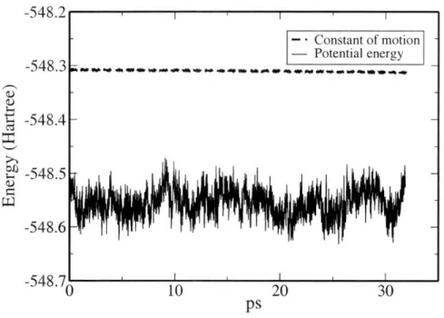
equili-bration runs for 32 water molecules at 325, 350, 375 and 400 K. . . . 45 3-4 Potential energy and constant of motion in a production run at 400 K. 46 3-5 Kinetic energy of the ions and the electrons in a production run at 400

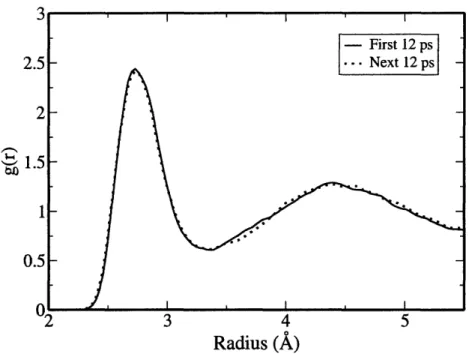
K . . . .. . 46 3-6 0-0 radial distribution functions calculated from the first and the next

12 ps of the simulation at 400 K. . ... . 47 3-7 0-0 radial distribution functions calculated from the production runs

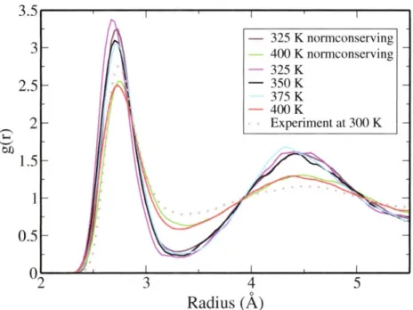
at 325 K, 350 K, 375 K and 400 K for ultrasoft and norm-conserving pseudopotentials. ... 50 3-8 O-D radial distribution functions calculated from simulations at 325

K, 350 K, 375 K and 400 K for ultrasoft and norm-conserving pseu-dopotentials... . .. .. .. . . .. ... . . . . .. . . . . .. . . 51 3-9 Mean square displacements calculated from simulations at 325 K, 350

(12)

3-10 0-0 radial distribution function for a Car-Parrinello simulations with 32 or 64 molecules. ... 54 3-11 0-0 radial distribution function for a classical (SPC) simulation with

64 or 1000 water molecules. ... 55 3-12 Power spectrum of deuterium atoms calculated from the velocity-velocity

correlation function. ... 56

4-1 A schematic diagram of inelastic X-ray scattering by an electron: a photon with energy h1wl and momentum kl hits an electron with initial energy El and momentum pi. The photon is scattered away with energy hw2 and momentum k2. . . .. . . 61

4-2 0-0 radial distribution functions from simulations at different thermo-dynamic state points and comparison with the experimental data at ambient condition. ... 67 4-3 The absolute Compton profiles for the simulations at 77 0C and 430 OC. 69 4-4 (a) Experimental Compton profile difference AJ(p) with respect to

the liquid reference state at different temperatures. (b) Theoretical Compton profile difference AJ(p) with respect to the liquid reference state at different temperatures. ... 70 4-5 The integration of the absolute value of the profile difference, ne, as a

function of temperature for simulations . ... 72 4-6 Procedure to calculate the Compton profiles at different nHB using a

model structure of 5 water molecules. . ... . 73 4-7 Compton profile differences for different nHB calculated from different

clusters with 77 "C as the reference state. . ... 74 4-8 n, as function of the number of H-bonds per molecule (nHB) ... 75

(13)

4-9 (a) snapshots of simulations at 200 OC, 300 OC and 430 "C. The color code represents water molecule connectivity. Blue: molecules net-worked with more than 5 other molecules; green: molecules netnet-worked with 2 to 5 other molecules; red: monomers. (b) Number of water molecules (y-axis) distributed in clusters of different sizes (x-axis) for various temperatures ... 77

5-1 Schematic diagram of the electron-transfer process. . ... 81 5-2 Diabatic free-energy surfaces for a typical electron-transfer reaction.. 82 5-3 Diabatic free-energy surfaces for Fe2+-Fe3+ electron transfer reaction

calculated using classical molecular dynamics simulations when the ions are 5.5

A apart. The figure is taken from Ref. [114] ...

90 5-4 Schematic diagram showing the division of the reorganization energy

contributions into inner and outer sphere. . ... 92 5-5 Procedure to calculate the inner-sphere and outer-sphere contributions

to the reorganization energy. . ... .... 93 5-6 Procedure used to calculate the diabatic free energy surfaces for

elec-tron transfer from first-principles molecular dynamics.... . . . . 96 5-7 The Fe-O radial distribution functions for Fe(2+r)+ solvated in water

with r=0, 0.25, 0.5, 0.75, 1. ... ... . 98 5-8 Diabatic free energy surfaces for ferrous-ferric electron transfer in the

special case when two ions are infinitely apart. . ... 99 5-9 The HOMO orbital charge density distribution in the case when one

hexa-aqua ferrous and one hexa-aqua ferric ions in the same unit cell. 100 5-10 The transferring electron can be localized at the desired location with

the appropriate sign of P' and value of fo ... 101 5-11 Charge density difference compared to DFT ground state charge

den-sity (calculated from ferrous and ferric ion clusters in separate cells), without (above) and with (below) penalty functional. . ... 104

(14)

5-12 Diabatic free energy surface for ferrous-ferric electron transfer when the two ions are 5.5 A apart... .. 106

A-1 The total energy profile as a function of the number of electrons in the

system .. . ... . . . .. .. 117 A-2 Uot as a function of Ui, for ferrous and ferric hexa-aqua ion clusters. 122 A-3 The potential energy, constant of motion and Fe-O radial distribution

functions of the simulation with ferrous ion and ferric solvated in 31 water m olecules ... 125

(15)

List of Tables

3.1 Structural properties of the water monomer and dimer and binding energy of the dimer, as obtained in DFT-PBE using ultrasoft or norm-conserving pseudopotentials, and compared to available experimental and theoretical results. ... 39

3.2 Vibrational frequencies of water monomer: vj, v2 and v3 are the

sym-metric stretching, bending and asymsym-metric modes, respectively. . . . 40

3.3 Vibrational frequencies of water dimer: vy, v2 and v3 are the symmetric stretching, bending and asymmetric stretching modes, respectively. . 40

3.4 Structural and dynamical parameters before and after the 10 ps mark, compared with the experimental results at 298 K. . ... . . 43 3.5 Details of the production runs ... 48 3.6 Summary of structural and dynamical properties of water at different

temperatures. ... 51

4.1 Temperatures and densities used in ab-initio simulations for different thermodynamics state points studied . ... 65 4.2 Comparison of self-diffusion coefficients between simulations and

(16)

4.3 Experimental and theoretical (after scaling of 0.73) ne, and theoretical nHB at different state points. The first column shows the experimental temperature and pressure at each state point. The theoretical temper-atures and pressures are the same as the experimental ones except in the first and the last state points shown below, which are (77 OC, 1 bar) and (430 OC, 300 bar). respectively. . ... 76 5.1 The energy gaps calculated with the penalty functional and the

"4-point" approach for different random cluster geometries. . ... 104 A.1 The dFe-o's of the relaxed structures for hexa-aqua ferrous and ferric

(17)

Chapter 1 Introduction

Electron-transfer reactions are one of the most ubiquitous processes in organic and inorganic redox reactions. They cover processes and applications as diverse as solar-energy conversion in the early steps of photosynthesis, oxidation-reduction reac-tions between a metallic electrode and solvated ions, and the I-V characteristics of molecular-electronics devices [1]. According to the seminal work by Marcus [2], fluctu-ations of the environment (solvent) are crucial in mediating the transfer of an electron from the reactants to the products. The central role played by the structure and dy-namics of the solvent (water in our case) requires also an extensive first-principles characterization of water and aqueous systems.

Water, due to its abundance on the planet and its role in many chemical reac-tions, has been widely studied both experimentally [3,4] and theoretically. Despite the effort devoted to this, many questions remain unanswered or controversial down to the average number of hydrogen bonds or the radial distribution functions of liq-uid water. The peculiar interplay of hydrogen bonding, glassy behavior, electronic structure, and of quantum-mechanical effects on the dynamics of the atomic nuclei make computer simulations challenging, and a great effort has been expended to build a comprehensive and consistent microscopic picture, and a link with observed macroscopic properties [5-22].

Computational studies based on molecular dynamics simulations have a long his-tory in the field. Simulations using force-fields models [5-10] have been successful at

(18)

reproducing many structural and dynamical properties of liquid water. However, em-pirical models rely on parameters which are determined by fits to known experimental data, or occasionally to ab-initio results. Their transferability to different environ-ments, or the ability to reproduce faithfully the microscopic characteristics of hydro-gen bonding, are often in question. Due to development of novel techniques [23-25] and the ever-increasing improvement in computational power, extensive molecular-dynamics simulations from first-principles are now possible. The increased accuracy and predictive power of these simulations allow studies of many systems with excellent quantitative accuracy, which had not been feasible before.

In this thesis, we first carry out extensive studies of the structural, dynamical and electrochemical properties of water and of aqueous systems using first-principles methods. The structural properties and binding energy of the water monomer and dimer are studied in details using density-functional theory, paired with a modern exchange-correlation functional (PBE). Although there has been a long-standing be-lief that the structural and dynamics from first-principles molecular simulations of water at ambient conditions are in excellent agreements with experiments, this pic-ture has recently been revised by a number of investigations [26, 27] including our own [28].

Our efforts have not been confined to studying water at ambient conditions. Due to the potential applications of water at supercritical regime (e.g. as a solvent in organic waste disposal), the microscopic properties of supercritical water are also of central interest. Despite numerous efforts, the hydrogen bonding structure of water at supercritical regime is also controversial. Neutron diffraction results have been interpreted differently: some authors [29,30] conclude that nHB - 0 above the critical point whereas others conclude that nHB is still sizable [31,32]. Other experimental techniques, such as X-ray diffraction [33], infrared spectroscopy [34], or NMR [35] point to a persistence of hydrogen bonds in supercritical water (SCW).

We combine here theoretical and experimental efforts to derive a robust measure of the hydrogen bonding structures from the ground-state electronic structure of the system, not from the ionic structure as it is done in the neutron and X-ray

(19)

Figure 1-1: Diabatic free-energy surfaces for a typical electron-transfer reaction.

diffractions. The electronic ground state can be unambiguously accessed in X-ray inelastic (Compton) scattering experiments and straight-forwardly calculated from our first-principles methods.

With these understandings of structure and dynamics of water, we then proceed to study electron-transfer reactions in aqueous environments. The key quantities of interest are the reaction rates (or, equivalently, the conductance) and the reaction pathways. Reaction rates, in the general scenario of Marcus theory [19,36,37], have a thermodynamic contribution (the classical Franck-Condon factor, broadly related to the free energy cost of a nuclear fluctuation that makes the donor and the acceptor levels degenerate in energy), and an electronic-structure, tunneling contribution (the Landau-Zener term, related to the overlap of the initial and final states).

According to the Marcus theory of electron transfer, which we will discuss in details in Chapter 5, electron tunneling would occurs only when the system is at the crossing point of the two free energy surfaces. As indicated in Fig. 1-1, a free energy barrier of AG* has to be overcome to reach the crossing point. In the limit of small

(20)

tunneling matrix element (diabatic limit), the reaction rate can be treated according to Fermi's golden rule,

2ir

kET = -IHDAI 2FC (1.1)

where HDA is the electronic coupling matrix element between the donor and the acceptor and FC is the Franck-Condon factor [36],

FC = exp(-(AGO + A)2/4AkBT) (4?rAkBT)1/2

where A and AGo are the reorganization energy and the free energy of reaction as indicated in Fig. 1-1. From the above equation, we can see that there are three parameters defining the electron-transfer rate in the diabatic limit, namely HDA, A

and AGo

There have been numerous studies of electron-transfer reactions in the context of Marcus theory. Most studies provide the correct qualitative picture but fail to describe the reactions with quantitative accuracy. This discrepancy is due to the inaccuracy of classical potentials in dealing with processes where there is a significant change in the electronic structure. In order to provide a better quantitative picture of electron-transfer reactions, we develop a novel approach to allow the study of electron-transfer reactions from first-principles molecular dynamics. Our approach involves extensive umbrella sampling of the solvent phase space and the introduction of a novel energy functional to calculate accurately both the ground and first excited state of electron-transfer reactions. With aqueous ferrous-ferric self-exchange as a paradigmatic example, we show how accurate the diabatic free energy surfaces can be obtained with excellent agreement with the experiments.

Last, in the appendix, we discuss a DFT + Hubbard U [38,39] approach targeted at correcting the over hybridization of localized orbitals that takes place at standard density-functional theory.

The thesis is organized as follows:

* Chapter 2, We describe the general computational techniques used in this re-search.

(21)

* Chapter 3, We present in details the simulations procedure and results of first-principles studies of water at ambient conditions.

* Chapter 4, X-ray inelastic scattering study of water at ambient and supercritical conditions are presented. We also derive a robust measure of the hydrogen bonding structure so that the average number of hydrogen bonds per molecule can be easily obtain from Compton scattering spectra of water in experiments. * Chapter 5, We present our approach to study electron-transfer reactions from first-principles molecular dynamics. Using aqueous ferrous-ferric self-exchange as a paradigmatic example, we present the full diabatic free-energy surfaces calculations from first-principles.

* Chapter 6, The works are summarized in the conclusions.

* Appendix A, We discuss the DFT + Hubbard U studies of strongly correlated systems and its implementation in Car-Parrinello molecular dynamics. We also study the effects of the Hubbard U corrections on the ferrous and ferric ions solvation in water.

(22)

(23)

Chapter 2 Computational techniques

2.1 Introduction

In this chapter, we will provide a brief review of the theoretical approaches and the approximations used in this research. Our work is based on the study of the properties of matters from first-principles. A calculation is said to be from first-principles if it relies on basic and established laws of nature without additional assumptions or special models. In studying the electronic properties of matters, the established law of nature is the Schroedinger's equation. Although the exact form of the Schroedinger's equation is known, getting the exact solution is almost impossible in realistic systems, due to the interactions between electrons. Many techniques have been developed to solve this equation via various approximations. Density-functional theory (DFT), which has become one of the most widely used first-principles techniques to efficiently solve the Schroedinger's equation, will be discussed in this Chapter. Although density-functional theory is, in principle, exact, in practice, its ability to describe correctly the properties depends on the accuracy of the exchange-correlation functionals used. the ability of the theory to correctly describe electronic properties of matters depends on the accuracy of the exchange-correlation functional. We will review briefly the more common approximations available.

In actual calculations, the wavefunctions have to be expanded in a basis set. One of the set most commonly used is the plane-wave basis set and we will discuss its use

(24)

and its advantages over others. The concepts of norm-conserving pseudopotentials and ultrasoft pseudopotentials to lower the computational costs in simulations will also be explained. We will then review the Car-Parrinello method, which greatly reduces the computational cost for finite temperature studies from first-principles molecular dynamics. Moreover, we will mention an extension to the technique to allow molecular dynamics at constant temperature.

2.2 Density-functional theory

In studying the electronic properties of matter, solving exactly the Schroedinger's equation is all we would need. A physical observable (0) can be calculated from the expectation value of a corresponding operator (0) through the relation, O = (TI~II), where T is the many-body eigenfunction of the Schroedinger's equation. For an isolated N-electron and M-atom system, the electronic wavefunctions can be calculated and all the physical properties can be described by the Schroedinger's equation,

HI({rs})'I({r,}) = E'({r,}), (2.1)

N 1 N M N

H({ri}) = T + Vne + Vee = V2) + ZI +Z (2.2)

2i

Iri

-RII+

r&j

H is the many-body Hamiltonian and T is antisymmetric due to fermion spin statis-tics. The ground-state wavefunction is the one that minimizes the energy and the corresponding energy is the ground-state energy. Although the above equation can, in principle, be solved exactly, the problem becomes practically unsolvable as the number of electrons increases. A very successful reformulation of the problem was in-troduced in 1964-65 by Hohenberg, Kohn and Sham [40,44] that provides a tractable approach to deal with the many-electron problem.

In particular, the first Hohenberg-Kohn theorem [40] states that if the ground state electronic density, no(3f, is known, the external potential acting on the elec-trons (i.e. the potential due to the electrostatic interaction with the ions) is also

(25)

uniquely determined, at least for the case with non-degenerate ground state. Since no(rj also determines the number of electrons in the system, the ground state many-body wavefunction, 90 is then uniquely defined, in principle, from any given no(r). Therefore, the total energy, besides being a functional of the ground state wavefunc-tion, can be written as a functional of the electronic density itself. Hohenberg and Kohn then introduced,

F[n(rj] (T It+ ~ee ~), (2.3)

E [n(rl] v(r--n(rdr + F[n(r-], (2.4)

where F[n(rl], which is an universal functional independent of the external potential, contains the kinetic energy and the electron-electron interaction term, and Ev[n(rj] is the total energy functional with the external potential included. In the above formula, F[n(r)] is defined only with v-representable charge densities. A density is v-representable if it is the density associated with the antisymmetric ground-state wavefunction of the interacting Hamiltonian (Eq. 2.2) with some external potential. The second Hohenberg-Kohn theorem [40] provides a variational principle,

Eo < E"[A((rj], (2.5)

for any trial v-representable electronic density such that f P(rjdr = N.

Note that many "reasonable" densities are not v-representable, but, as proposed by Levy [41,42] and Lieb [43], density-functional theory can be reformulated so that the electronic densities satisfy a weaker condition, of N-representability. A density is N-representable if it can be obtained from some antisymmetric wavefunction (not nec-essarily the ground state wavefunction in some external potential). N-representability is satisfied for any reasonable density. With the Levy-Lieb constrained-search defini-tion,

F[n(rj] = min_,n( (I( It + V~eel). (2.6) The universal functional F[n(r-)] is now defined for any N-representable charge

(26)

den-sity. Note that there can be many I's that give the same N-representable n(F) and F[n(rj] is defined as the minimum expectation value of T + Ve searching over all the antisymmetric wavefunctions that integrate to n(r).

The determination of the ground state is in principle greatly simplified by Eq. 2.5; instead of minimizing the energy functional with respect to the many-body wave-function, we can now minimize the energy functional with respect to the electronic density. However, the universal functional F[n(')] is unknown in practice and this prevents any real applications. Kohn and Sham [44] provided a practical solution by introducing the concept of a noninteracting-electron reference system,

N N

Hs

=

Z(-

v)

+

Z v(r), (2.7)

i i

where the potential v,(ri) is such that the ground state density is exactly the same as the interacting system. For the noninteracting system, the exact ground state wavefunction is the Slater determinant,

1

9, = det['lI1 2 ... PN], (2.8)

where the 0i are the N lowest eigenstates of the noninteracting Hamiltonian. There-fore, the problem is now shifted from finding the correct n(rj to finding the correct

noninteracting Hamiltonian. We can rewrite the universal energy functional as, F[n(rl] = T,[n(l)] + EH[n(rl] + Exc[n(rj], (2.9)

where

Exc[n(rj] - T[n(rl] - T,[n(rl] + Vee[n(rl] - EH[n(rj], (2.10)

with T[n(r)] the kinetic energy of the independent electrons Hamiltonian, EH[n(r-)] the Hartree energy and Eýc[n(r-] the exchange-correlation energy that contains the difference between T and T, (presumably fairly small), and the non-classical part of Vee[n(r1]. Functional minimization is performed according to the Euler-Lagrange

(27)

equation,

/i = ZAijy, (2.11)

where the right-hand-side comes from the orthogonality constraint on the Kohn-Sham wavefunctions and

1 2 f n(r')

HT = [(---V) + v(r- +

dr ' +

_vxc(rj],

_(2.12)

2 r _r_

-with the exchange-correlation potential

V 6 E c [ n ()rj ]

vc(r =

_{6n (rj}

(2.13)

Since the potential on the electrons depends on the charge density via the Hartree and the exchange-correlation terms, the equation has to be solved self-consistently. The Kohn-Sham approach is also, in principle, exact, but still requires the knowledge of Exc. Finding more and more accurate E.c is an active field of research.

2.3 Functionals for exchange and correlation

The crucial quantity in the Kohn-Sham approach is the exchange-correlation energy, which is expressed as a functional of the charge density Exc[n(rj]. As discussed in the Kohn and Sham's seminal paper [44I, by explicitly separating out the independent-particle kinetic energy and the long-range Hartree terms, the remaining exchange-correlation functional Exc[n(r-] can be reasonably approximated as a local or nearly local functional density. They pointed out that electrons in solid can often be con-sidered close to the limit of the homogeneous electron gas. In this limit, the effects of exchange and correlation can be treated as local in character, and therefore, the correlation functionals becomes an integral over all space with the exchange-correlation energy density at each point assumed to be the same as in a homogeneous

(28)

electron gas with that density,

EFcDA[n(rj] = d rn( c (n(I' ). (2.14)

This is the local density approximation (LDA). In the case of studying a magnetic system, the spin densities nt_{(rj and n((rf are not equivalent at every point in the}

system. An extension to LDA to study magnetic systems is the local spin density approximation (LSDA) where,

EfsDA[nt_{(r), n(r)]} ₌

J

_d3 _rn(r-rhzf _(nt_{(r), nt(r-))}

= d3rn(rfE* (nt (ri)n (r)) + Eahm(nft(rl, n (r).(2.15)

The exchange-correlation energy density can subsequently be separated into the ex-change energy and the correlation energy density. The exex-change energy of the homo-geneous gas is given by a simple analytical form using the Dirac exchange formula [45],

Eh" (nt (r, n J(rj))=- (- 6nt(r-) 1/3 - n (r ' )

3. (2.16)

T

4 i4

4 7r

On the other hand, the correlation energy density has been accurately calculated for the homogeneous electron gas as a function of density using high precision using Quantum Monte Carlo techniques [46].

The first step beyond the local approximation is a functional of the magnitude of the gradient of the density

IVnUI

at each point. The term generalized-gradient approximation (GGA) denotes various ways to include this dependence,

EGcGA [nt(?, n(f] = df rn(frExc(n ,'(rj, (I,

Vn( l|, Vn(r'))l

(2.17) Numerous forms for the GGA exchange-correlation functionals have been proposed, and among them, the most widely used functionals are B88 [47], PW91 [48], BLYP [49, 50] and PBE [51]. The generalized-gradient approximations show improvements over LSDA in many chemical problems, and therefore GGAs are widely adopted by the

(29)

chemistry community. However, every approximation has its limitations. Among the most serious faults is the spurious self-interaction present in most exchange-correlation functionals. In the Hartree-Fock approximation, the unphysical self-interaction term in the Hartree interaction is exactly canceled by the non-local exchange interaction. However, this cancellation is only approximate in most exchange-correlation func-tionals. This self-interaction effect is negligible in the homogeneous gas but large in cases with localized charge density, for example the d-electrons in transition metals. In Appendix A, we will actually look into a DFT + Hubbard U approach and discuss how it can better describe the physical properties of transition metal complexes.

2.4 Plane-wave basis set

In solving for the Kohn-Sham wavefunctions, it is necessary to expand them in a basis set. Many choices are possible, including atomic orbitals, Gaussians, linearized augmented plane wave (LAPW) and plane waves. The plane-wave basis set is most commonly used in extended systems with periodic boundary conditions. The use of a plane wave (PW) basis set has a number of advantages over other choices, including the simplicity of the basis functions, which make no assumptions regarding the form of the solution, the absence of basis set superposition error, and the ability to efficiently calculate forces on atoms. Moreover, full convergence of the forces acting on the ions with respect to the basis set is easily achieved with plane waves, and no Pulay forces arise in the dynamics, since the basis set is independent of the atomic positions.

Despite the advantages of using plane-waves, plane-waves with continuous values of the k-vector are, in principle, needed to fully represent a wavefunction. However, the use of periodic boundary conditions together with the Bloch theorem allow us to simplify the expansion. According to Bloch theorem, the wavefunctions can be written as Bloch wavefunctions,

(30)

In order to satisfy periodic-boundary conditions, the Bloch wavefunctions with quan-tum number k can be expanded in a discrete set of plane waves with k-vector (k+G), where G is the set of reciprocal lattice vectors. The set of values of k-vectors needed to represent a wavefunction now changes from continuous to discrete, but still infinite. In practice, the set of plane waves is restricted to a sphere in reciprocal space most conveniently represented in terms of a cut-off energy, Ect, such that for all values of G used in the expansion,

<h Ecut

(2.19) 2me

The choice of Ect depends on how structured wavefunctions are. Usually, to represent accurately the wavefunctions near the ionic cores, a large number of plane waves would be needed, making simulations very expensive computationally. The pseudopotential approximation, which we discuss in the next section, provides a solution to smooth the wavefunction around the core region and, therefore, requires a significant smaller number of plane waves.

2.5 Pseudopotential

Electrons in matter can be broadly categorized into two types - core electrons, which are strongly localized in the closed inner atomic shells, and valence electrons, which exist also outside the core. Since the potential in the region close to an atomic nucleus varies as 1_{, which diverges as r -- 0, an extremely large number of plane}

waves would be needed to expand the core electron wavefunctions and the valence electrons wavefunctions around the core region. This large number of plane waves would make the computational cost extremely high.

The use of pseudopotential approximation is a way to solve this problem, by re-moving the core electrons and replacing the interaction between the core and the valence electrons (vi"o(rf)) by a weaker pseudopotential with core electron screen-ing (vPS(rf) [52] (Fig. 2-1). Since most physical properties are determined by the valence electrons, this treatment is able to greatly reduce the computational cost,

(31)

r(' _PS. !I _I

O-OO

r)

Ion

Figure 2-1: An illustration of the concept of pseudopotential approximations. while describing physical properties with high accuracy. With this treatment, the valence pseudo-wavefunctions are smoother and nodeless in the core region and are identical to the real wavefunctions outside the core region. The computational cost in calculations using pseudopotentials is reduced in two ways. Firstly, the number of wavefunctions needed in a calculation is reduced by removing the core electrons. Sec-ondly, the valence wavefunctions are smoother within the core region and fewer plane waves are needed to adequately describe the valence wavefunctions. To ensure that a pseudopotential calculation reproduces the same energy differences as an all-electron calculation, it is necessary for the normalized pseudo-wavefunctions to be identical to the normalized all-electron wavefunctions outside the core. This condition is called 'norm-conservation'.

2.6 Ultrasoft pseudopotential

Ultrasoft pseudopotentials, developed by Vanderbilt [53], further relax the norm-conserving constraint. With this flexibility, ultrasoft pseudopotentials attain much smoother (softer) pseudo-wavefunctions and therefore can use considerably fewer

(32)

plane waves for calculations with the same accuracy. In this scheme the total va-lence density n(rJ is partitioned into hard and soft contributions,

n(ri =

Zr

5n(rJ;12_{+ Qij(rJ (On I ýj) (AI n) 1}

(2.20)

where ýi's are projector functions that depend on the ionic positions, and the aug-mentation function Qij(r) are given by

Qi,(r) = Oi* M 10i M - Of* M j (I (2.21)

where #i(i) are the all-electron wavefunctions, and 0i( ) are ultrasoft wavefunctions constructed without satisfying the norm-conserving condition Qi (j( = 0 . Also, the

orthonormality condition takes on a generalized form

(<i S({R,})i¢>) = 6ij,

(2.22)

where S({RI}) depends on the ionic positions through I/i) and is defined as, S({RI}) = 1i) + E qij (j ,

with,

qij =

f

Qij(rdr.

2.7 Car-Parrinello molecular dynamics

In performing molecular dynamics simulations, the motion of the atoms are described by the Lagrangian

C = T- - V. (2.25)

(2.23)

(33)

T and V are the kinetic and potential energies of the atoms. The Newton equations of motion can be obtained by minimizing the action (S =

f

£dt),

d (O& 0

dt ORI ORI

d2 RI dV

mI dt2 _d _(2.26)

dt2

'dRI

where R, is the position of atom I. In actual simulations, the trajectories of the atoms are obtained from the numerical integration of the equations of motion with a finite timestep 6t. The forces of on atoms, i.e. the right hand side of the equation of motion, are calculated in classical molecular dynamics from classical force-fields. However, classical force-fields usually contain experimentally fitted parameters to a particular condition, and the transferability and accuracy are usually in questions. A more accurate approach to obtain forces on atoms would be to calculate them quantum-mechanically (i.e. from first-principles). In the Born-Oppenheimer approximation, the ions move on the potential energy surface of the electronic ground state V =

(IF lHI I), where H is the Hamiltonian. The right hand side on the equations of motion now becomes

dV d( -I ')

dRI dRI

ORFI •RI

oRI

EOft

'a'>

<'o

fR

-E0

' '

_OR,

s'

_ORI

IF)

= -(~ I

I)

=

-(

)'I

),

(2.27)

where V is the operator for the external potential acting on the electrons, which is the only RI-dependent term in Hf. This is the Hellmann-Feynman theorem, which makes the calculation of forces a lot simpler, since the forces on atoms can now be calculated without the computation of the derivative of the wavefunction with respect to the positions of atoms and all is needed is the analytical form of d. Despite this

(34)

simplifications, the calculation of forces on atoms quantum-mechanically is still very time-consuming since it requires the computation of the ground state wavefunction at every timestep.

In 1985, Car and Parrinello [23-25] introduced a different approach to significantly lower the computational costs in performing first-principles molecular dynamics simu-lations. In this method, the ground state wavefunctions (i.e. the Kohn-Sham orbitals) are allowed to evolve simultaneously with the ions and the computation of the ground state wavefunctions is not needed at every timestep. The dynamics of the ions and the wavefunctions are described by the extended Lagrangian:

£cP = P fi Jdr

Ii

(r)+ 2 MIR - EKS [{'i}, {RI}]

i I

+

Aij

(f

dr'V* (r)

j

(r)

-

56ij) ,

(2.28)

ij

where EKS[{bi}, {RJ}] is the DFT energy functional and the 'i are the Kohn-Sham orbitals. The equation of motions for the ions and wavefunctions are, respectively,

dEKS[10i i

JRIJ]

MIR = dE [{ , {R(2.29) dRI

S 6EKs[{ i}, {RI}]

PIAi = - 6¢* + E Aijoj. (2.30)

The Kohn-Sham orbitals are allowed to evolve as classical degrees of freedom with the inertial parameters pi. The Lagrange multiplier Aij restricts the evolution of the wavefunctions to preserve the orthonormality. In performing Car-Parrinello molecular dynamics, the wavefunctions are relaxed to the ground state at a fixed set of ionic positions and then the ions are allowed to move according to the equations of motion. The electronic wavefunctions adiabatically follow the motion of the ions, with some small oscillations about the electronic ground state (Born-Oppenheimer surface). The electronic wavefunctions will have a "fictitious" kinetic energy associated with their motion and the fictitious mass pi. By choosing a small enough pi, the motion of the wavefunctions will be very fast relative to the motion of the ions and the wavefunctions

(35)

will stay very close to the instantaneous ground state.

Moreover, to ensure the wavefunctions stay close to the ground state in the course of the simulation, the ionic degrees of freedom need to be adiabatically separated from the electronic degrees of freedom so that the ionic dynamics would not heat up the "fictitious" electronic dynamics. This is achieved by ensuring that the frequency spectra of the electronic wavefunctions and the ions are well separated from one another; this condition can always be satisfied if there exists an energy gap between the occupied and unoccupied Kohn-Sham orbitals. Within a harmonic approximation, the lowest frequency of oscillation of the wavefunctions about the ground state may be written as

W= = 2(- ) (2.31)

where Ei and ej are the eigenvalues of the highest occupied and the lowest unoccupied

orbitals respectively. Therefore, a small enough pi is chosen so that wo is significantly larger than the highest ionic vibrational frequency so that the exchange of energy between the ionic and the electronic degrees of freedom is practically zero. However, a small pi requires a small timestep to correctly integrate the equations of motion for the wavefunctions. Special care is needed to choose the value of ui to obtain an optimal balance between the accuracy and the speed of the simulations.

2.8 Extended Lagrangian methods for molecular

dynamics in different ensembles

In the above discussion of the Car-Parrinello extended Lagrangian, the system is implicitly assumed to be in the micro-canonical (NVE) ensemble. Often, it is more convenient to fix the temperature rather than the total energy throughout the sim-ulation. While the temperature is an intensive quantity, it is related to its extensive counterpart (kinetic energy of the ions) by

2 Pi

T = -EkinNkB

₃

= 3 B p (2.32)

(36)

In this work, we adopt the integral thermostat method (or Nose-Hoover thermo-stat [54-57]) to control the temperature on the ions. The Nose-Hoover thermothermo-stat introduces additional degrees of freedom into the system's Hamiltonian, that becomes,

N 2 2

H = + V(r") + + (3N + 1)kBTln(s) (2.33)

i=2ms 2Q

where s is the additional degree of freedom and T is the target temperature. The equation for the additional degree of freedom evolves together with original spatial coordinates and momenta. Physically, the Nose-Hoover thermostat acts as a heat reservoir, with which the system can exchange energy, so that temperature (i.e. the total kinetic energy of ions) fluctuates around a target value. In some systems with small HOMO-LUMO gaps that it is not practical to choose a small enough "fictitious" mass to adiabatically separate the ionic and electronic degrees of freedom, a thermo-stat can be! applied to the electronic degrees of freedom so that the wavefunctions do not heat up and stay close to the Born-Oppenheimer surface.

(37)

Chapter 3 Static and dynamical properties

of

heavy water at ambient conditions

from.

first-principles molecular

dynamics

3.1 Introduction

Water, due to its abundance on the planet and its role in many of the organic and inorganic chemical processes, has been studied extensively and for decades both at the theoretical and at the experimental level [3-18,58]. In the last two decades, numerous ab-initio simulations on water have appeared [11-18], showing good agreement with experiments for the structural and dynamical data. However, this good agreement has recently been challenged by a number of investigations [26, 27] including our own [28, 59].

We have undertaken an extensive investigation of the static and dynamical prop-erties of water, to ascertain its phase stability around ambient conditions as predicted by first-principles molecular dynamics. Particular care has been given to the statis-tical accuracy of the results, assuring that the time scales and length scales of the

(38)

simulations were chosen appropriately for the given conditions.

In this chapter, we will first detail all the technical aspects of our simulations. Then, we will surveys the static and vibrational properties of the water molecule and the water dimer in vacuum, at the GGA-PBE [51] density-functional level. We will also discuss the extensive liquid water simulations, performed with Car-Parrinello molecular dynamics, in the temperature range between 325 K and 400 K. Moreover, we will discuss the limitations of this approach, and some of the possible reasons to explain the remaining discrepancies with experimental results.

3.2 Technical Details

The structural and vibrational properties of the water monomer and dimer and the binding energy of the dimer have been calculated using density-functional theory in the generalized-gradient approximation and the total energy pseudopotential method, and density-functional perturbation theory [60], as implemented in PWscf of our electronic structure package [61]. We performed separate calculations using either norm-conserving pseudopotentials for both the hydrogen and the oxygen, or ultrasoft ones. These same pseudopotentials were also used for the norm-conserving or ultra-soft molecular dynamics simulations. In particular, the O Troullier-Martins norm-conserving pseudopotential [62] was generated using the FHI98PP package [63] with core radii for the s, p and d components of 1.25 a.u., 1.25 a.u., and 1.4 a.u. re-spectively. The Troullier-Martins hydrogen pseudopotential was generated using the Atom code [64] with a core radius for the s component of 0.8 a.u. The ultrasoft pseu-dopotentials were taken from the standard PWscf distribution [65]. The Kohn-Sham orbitals and charge density have been expanded in plane waves up to a kinetic energy cutoff of 25 and 200 Ry (respectively) for the ultrasoft case, and of 80 Ry and 320 Ry for the norm-conserving case. A cubic supercell of side 30 a.u. was used; interaction with periodic images is negligible [66] with this unit cell size.

(39)

Table 3.1: Structural properties of the water monomer and dimer and binding energy of the dimer, as obtained in DFT-PBE using ultrasoft or norm-conserving pseudopotentials, and compared to available experimental and theoretical results.

PBE US PBE NC PBE NC Experiments BLYP (This work) (This work) (Ref [71]) (Ref. [67-70]) (Ref. [66])

ZHOH 104.60 104.20 104.20 104.50 104.40 doH(A) 0.98 0.97 0.97 0.96 0.97 ZOHO 1730 1720 1740 1740 1730 doo(A) 2.89 2.88 2.90 2.98 2.95 Edimer -23.2 -23.8 -21.4 -22.8 -18 (kJ/mol)

3.3 Water monomer and dimer: Structural and

Vibrational Properties

The equilibrium structures and energetics are summarized in Table 3.1. We have included published results [66] using the BLYP functional for comparison. Both ultrasoft and norm-conserving PBE density functionals show very good agreement with experimental values. In particular, the PBE results have a dimer binding energy in closer agreement to the experiments than BLYP; the binding energy in this latter case is too weak by 4 kJ/mol, and exhibits a longer 0-0 distance.

Table 3.2 and 3.3 show respectively the vibrational frequencies of the water monomer and dimer in vacuum. In this calculation, a hydrogen mass of 1 a.m.u. was used (as opposed to the 2 a.m.u. mass used for the dynamical simulations of heavy wa-ter). The calculations of the vibrational frequencies were performed using density functional perturbation theory using a cubic cell of size (30 a.u.)3. To achieve a con-vergence of a few cm- 1 in the frequencies, cutoffs of 35 Ryd and 420 Ryd were used for wavefunctions and charge densities, respectively, in the ultrasoft case and, in the norm-conserving case, 100 Ryd and 400 Ryd were used. As shown in Table 3.2 and 3.3, the PBE functional gives intramolecular stretching modes that are in general blue-shifted compared to BLYP and experimental results. In the calculations for the dimer, the libration modes are also higher for the PBE functionals then those given

(40)

Table 3.2: Vibrational frequencies of water monomer: vy, v2 and u3 are the symmetric

stretching, bending and asymmetric modes, respectively. PBE (US) PBE (NC) Expt [67] BLYP [66] v, (cm- 1) 3781 3704 3657 3567 v2 (cm-1') 1573 1599 1595 1585

u3(cm-1) 3908 3816 3756 3663

Table 3.3: Vibrational frequencies of water dimer: vj, v2 and v3 are the symmetric stretching, bending and asymmetric stretching modes, respectively. Proton acceptor and donor molecules are denoted as (A) and (D). v(Hb) are the two libration modes between molecules and v(O- O) is the hydrogen-bond stretching mode.

PBE (US) PBE (NC) Expt [67-70] BLYP [66] v, (A)(cm- 1) 3778 3695 3622 3577 v2(A)(cm'- ) 1570 1596 1600 1593 v3 (A)(cm- 1₎ ₃₉₀₁ ₃₈₀₄ ₃₇₁₄ ₃₆₇₅ v (D) (cm- ') 3601 3532 3548 3446 v2(D)(cm- 1) 1593 1616 1618 1616 v3(D)(cm- 1) 3871 3781 3698 3647 v(Hb)(cm-1) 666 644 520 600 v(Hb)(cm- 1) 379 378 320 333 v(O - O)(cm-1) 202 196 243 214

by experiments and BLYP. We note in passing that the errors (especially the low energy ones) are slightly larger than usually We will return to this point in a later section.

on these frequencies expected from DFT.

3.4 Liquid water simulations

3.4.1 Liquid water simulation at 325 K

Simulation Details

In this first simulation, we used a body-centered-cubic supercell with 32 heavy water molecules, periodic boundary conditions, and the volume corresponding to the exper-imental [72] density of 1.0957 g/cm3 _{at 325 K. A body-centered-cubic supercell strikes}

(41)

the optimal balance, for a given volume, in the distance between a molecule and its periodic neighbors, and the number of these periodic neighbors. Ultrasoft pseudopo-tentials were first used, as detailed in the previous section, with plane-wave kinetic energy cutoffs of 25 Ry (wavefunctions) and 200 Ry (charge densities). The deuterium mass was used in place of hydrogen to allow for a larger timestep of integration. It should be noted that for classical ions this choice does not affect thermodynamic properties such as the melting temperature (the momentum integrals for the kinetic energy factor out in the Boltzmann averages). Of course, dynamical properties such as the diffusion coefficient will be affected by our choice of heavier ions. Extensive experimental data for deuterated (heavy) water are in any case widely available.

The wavefunction fictitious mass (p) is chosen to be 700 a.u.; this results in a factor of -14 between the average kinetic energy of the ions and that of the electrons. A timestep of 10 a.u. was used to integrate the electron and ionic equations of motions. This combined choice of parameters allows for roughly 25 ps of simulation time without a significant drift in the kinetic energy of wavefunctions and the constant of motion for the Lagrangian (2.28). Our choice of fictitious mass is consistent with the ratio p/M < 1 for heavy water molecules suggested by Grossman et al. [26] and assures that the physical properties are not influenced by the electronic degrees of freedom. Our initial configuration was obtained from a comparatively short 1.2 ps simulation at twice the value of the target temperature (650 K instead of 325 K); a restart with zero initial velocities was then performed at 325 K, with the temperature controlled by a single Nose-Hoover thermostat on the ions (no electronic thermostat is applied in any of the simulations).

Results

The thermostat stabilizes quickly (-1 ps) the temperature around the target value of 325 K, with the usual fluctuations due to small size of the system. However, the system is still far from equilibrium; this can be clearly observed by looking at the time evolution of the radial distribution function (RDF) and mean square displace-ments (MSDs). We plot in Fig. 3-1 the MSDs of the oxygen atoms as a function of

(42)

time. For the first 10 ps, the water molecules diffuse with a velocity comparable with experimental data; after 10 ps, a sharp drop in diffusivity is observed, accompanied by a distinctive sharpening of the features in the oxygen-oxygen radial distribution function (see Fig. 3-2). The radial distribution functions was calculated from the infinite bulk system by repeating the unit cell in all directions. This means that molecules up to 5.5 A in a 32-molecule cell are inequivalent. As we move beyond this cutoff distance, the radial distribution functions will include both molecules that are inequivalent, and some that are equivalent. The statistical accuracy is going to be gradually, but slowly, affected. In this graph, and most of the latter figures, we plot radial distribution functions only up to 5.5 A(but see e.g. Fig. 10 for a discussion of the finite-size effects).

The potential energy for the dynamics (Fig. 3-1) also drifts downward in these first 10 ps, and stabilizes afterward. We calculated the self-diffusion coefficient (Dself) from the Einstein relation (in 3 dimensions):

6Delf = lim

(Iri

(t) - ri (0)12). (3.1)

The structural and dynamical properties before and after this 10 ps mark are sum-marized in Table 3.4; experimental values at 298 K are included for comparison. All these observation conjure to a picture in which the system takes at least 10 ps to reach a reasonably thermalized state, in a process somewhat reminiscent of a glass transition. Although the time needed for equilibration will be dependent on the initial conditions, these preliminary result suggests that simulation times in the order of ten of picoseconds might be need to calculate well-converged thermodynamic observables.

Once the initial thermalization trajectory was discarded from our averages, we obtained a self-diffusion coefficient one order of magnitude smaller than the experi-mental value measured at room temperature. This result, combined with the clear over-structuring of the oxygen-oxygen radial distribution function goo(r), indicates that our system has reached a "frozen" equilibrium state very different from what expected for liquid water (strictly speaking, a system with a finite and small number

(43)

(1 rJ -548.32 -548.4 -548.48 -548.56q -548.64 T 0548.72

Figure 3-1: Mean square displacement and potential energy as a function of time for our first 32-water molecules simulations at 325 K. A: Diffusive region in the first stage of the simulation. B: After about 10 ps diffusivity drops abruptly.

Table 3.4: Structural a compared wi

nd dynamical parameters before and after the 10 ps mark, th the experimental results at 298 K.

g(r),maz D (cm /s) Before 2.82 1.5 x 10- 5

After 3.21 0.14 x 10- 5 Expt [4, 72] 2.75 2.0 x 10- 5

of inequivalent atoms or molecules will never undergo a phase transition).

These considerations indicates the need to assess accurately the phase stability of liquid water as obtained from first-principle molecular dynamics. At the same time, they point out the requirement of long simulation times, and a careful analysis of the technical details of the simulations.

Aqueous systems from first-principles : structure, dynamics and electron-transfer reactions

Aqueous systems from first-principles:

dynamics and electron-transfer reactions

by

Patrick Hoi Land Sit

MPhys. in Physics, University of Oxford, UK. 2000

Submitted to the Department of Physics

in partial fulfillment of the requirements for the degree of

Doctor of Philosophy in Physics

at the

MASSACHUSETTS INSTITUTE OF TECHNOLOGY

@

Massachusetts

July 2006

Institute of Technology 2006. All rights reserved.

Author ...

...

r...

Department of Physics

July, 2006

Certified by. ...

.

..

Nicola Marzari

Associate Professor, Department of Materials Science and Engineering

Thesis Supervisor

Aciepted by...

.. :...

..-.

Thomas J

reytak

Professor (If Physics

JUL 0 2 2007

LIBRARIES

ARCHIVES

f

structure,

Aqueous systems from first-principles: structure, dynamics

and electron-transfer reactions

by

Patrick Hoi Land Sit

Abstract

Acknowledgments

Contents

List of Figures

A apart. The figure is taken from Ref. [114] ...

List of Tables

Chapter 1

Introduction

Chapter 2

Computational techniques

2.1

Introduction

2.2

Density-functional theory

Iri

r&j

Hs

=

Z(-

v)

+

HT = [(---V) + v(r- +

vxc(rj],

6n (rj

2.3

Functionals for exchange and correlation

J

T

4 i4

4 7r

IVnUI

Vn( l|, Vn(r'))l

2.4

Plane-wave basis set

2.5

Pseudopotential

O-OO

r)

2.6

_vxc(rj],

_{6n (rj}

_OR,

_ORI

₃