Color imaging segmentation for automatic alignment of Atomic Force Microscope

Color Image Segmentation for Automatic Alignment of Atomic Force Microscope.

by

Pradya Prempraneerach B.S., Mechanical Engineering Carnegie Mellon University, 1998 Submitted to the Department of Mechanical

in Partial Fulfillment of the Requirements for the Degree of Master of Science in Mechanical Engineering

at the

Massachusetts Institute of Technology February 2001

© 2001 Massachusetts Institute of Technology

All rights reserved

ENPI

Signature of Author...

Certified by...

V I

...

Department of Mechanical Engineering February 1, 2001

-fV

Prof. Kamal Youcef-Toumi Professor, Mechanical Engineering Thesis Supervisor

A ccepted by ...

Dr. Ain A. Sonin Professor, Mechanical Engineering Chairperson, Departmental Committee on Graduate Students

MASSA C HLUS EUTS INaTITUTE OF TECHNOLOGY

JAN

16 2002

Color Image Segmentation for Automatic Alignment of Atomic Force

Microscope.

by

Pradya Prempraneerach

Submitted to the Department of Mechanical Engineering on February 1, 2001 in Partial Fulfillment of the Requirements for the

Degree of Master of Science in Mechanical Engineering

ABSTRACT

Traditionally, an alignment process of the Atomic Force Microscopy's (AFM) probe and sample manually and accurately is slow and tedious procedure. To be able to carry out this procedure repeatedly in large volume process, an image recognition system is needed to process this procedure autonomously. An image recognition system is mainly composed of two separated parts, segmentation and classification methods.

In this research, a new color-image segmentation procedure is proposed to overcome the difficulty of using only gray-scale image segmentation and over-segmentation. To extract color information similar to human perception, a perceptually uniform color space and to separate a chromatic value from an achromatic value,

CIELUV and IHS color spaces are used as basis dimensions to obtain the coarse

segmentation. The intervals of each dimension: intensity, hue and saturation are determined by the histogram-based segmentation with our valley-seeking technique. Then the proposed three-dimensional clustering method combines this coarse structure into distinct classes corresponding to objects' region in the image.

Furthermore, the artificial neural networks is employed as classification method. The training and recognition processes of desired images are applied using unsupervised learning neural networks: competitive learning algorithm. Typically, images acquired from the AFM are restricted only to similarity and affine projections so that main deformations of the objects are planar translation, rotation and scaling. The segmentation method can identify the position of samples, while the objects' orientation must be correctly adjusted before processing the recognition algorithm.

Thesis Supervisor: Prof. Kamal Youcef-Toumi Title : Professor of Mechanical Engineering

Acknowledgements

These thesis and research become successful with many supports of several persons, whom I am really appreciated and would like to thank here. First of all, my advisor, Prof. Kamal Youcef-Toumi, I would like to thank him for giving me an opportunity to work on this exciting research topic and also his motivation and suggestions to make this research become possible. It has been an invaluable experience for me to accomplish this project.

Furthermore, I would like to extend my thanks to my family, especially my father, mother and grandmother for supporting and taking care of me through my life. I am very grateful to have them as my family. Also, I like to thank my sister for her thoughtfulness and cheer.

In addition, I would like to give special thanks to my friends, both in Thailand and at MIT. I would like to thank my lab-mates, particularly Bernardo D. Aumond, El Rifai Osamah M, and Namik Yilmaz, in the "Mechatronics Research Laboratory" for many recommendations on how to operate the equipment as well as the software and a friendly-working environment. I also like to thank Susan Brown for several suggestions on editing this thesis. Lastly, I like to give a special thank to my friend, who I do not want to mention name here, in Thailand for understanding and support me during this time.

ABSTRACT ACKNOWLEDGEMENTS TABLE OF CONTENTS Chapte Chapt Chapt Chapt

-Conclusion and future works

Conclusion

Further improvement and future works

Appendix A: Introduction of Morphological operations. Table of Contents 2 3 4-5 r 1: - Introduction 1.1) Introduction

1.2) Background and Motivation

1.3) Objective of this research 1.4) Thesis Organization

-r 2: -Recognition System and Comparison 2.1) Introduction

2.2) Recognition system

2.3) Segmentation algorithm

2.4) Feature selection for segmentation 2.5) Clustering

2.6) Summary

-r3: - Science of color

3.1) Science of color

3.2) The CIE system

3.3) Uniform Color spaces and color difference formulas 3.4) Different color space for representing color image 3.5) Summary

r 4: -Proposed Segmentation Technique

4.1) Introduction

4.2) Histogram-based segmentation

4.3) Filtering: Morphological filtering operations and Edge-preserving filtering operation 4.4) Histogram valley-seeking technique

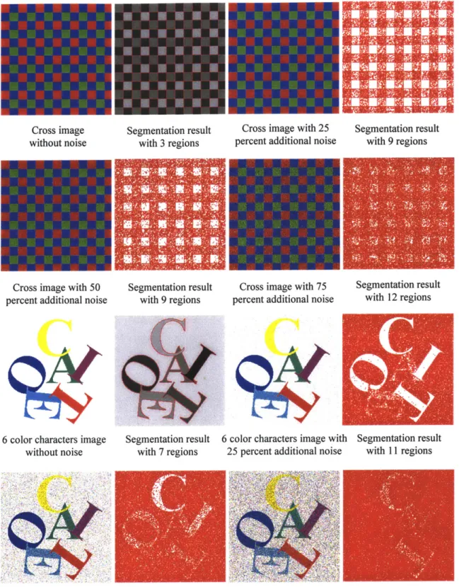
4.5) Three-dimensional color-space cluster detection 4.6) Experimental results, discussion and evaluation

4.6.1) Evaluation measurement function 4.6.2) Experimental results and evaluation 4.6.3) Segmentation results of natural scenes 4.7) Summary 6-8 8-10 10-11 11 12 12-13 13-15 15-18 18 19 20 20-31 31-35 35-45 45-46 47-48 48-52 52-56 56-62 62-67 67-76 76-77 77-92 93-103 104-106 107-108 109-110 110-111 112-115 Chapter 5: 5.1) 5.2)

Appendix B:

B.1)

B.2) B.3) B.4)

Classification -Neural Networks

Introduction to Neural Networks Competitive learning Neural Networks Experimental results and discussion

Summary

Appendix C: Segmentation program References 116-117 117-122 123-127 128 129-176 177-179

Chapter 1: - Introduction

1.1: Introduction

For the past decade, profilometry and instrumentation techniques for imaging material surface at atomic level with outstanding accuracy have been developed rapidly.

All these techniques are known as Scanning Probe Microscopy (SPM), including

Scanning Tunneling Microscopy (STM), Atomic Force Microscopy (AFM) and etc. However, in this research, the main focus is only on the AFM. The AFM operation is carried out by detection of a displacement of cantilever's probe due to an inter-atomic interaction known as van der Waals forces between the probe and the samples' surface, while the probe scans the samples' surface. Generally, the AFM cantilevers have dimensions in the order of 100 micrometers and the tip of the probe that is mounted on the cantilever is usually in the 10 micrometers range. The main components of the AFM are the cantilever with mounted probe, a large photodetector array for measuring the cantilevers' deflection, sample holder and positioner, a piezoelectric actuator, and a control system to maintain the position of the probe with the samples' surface. In addition, the AFM in our experimental setup also consists of a ccd camera, motorized and non-stacked x-y translation stages and z-axis motorized stage for a visual purpose of aligning and positioning the probe over certain samples' part to be scanned.

Traditionally, a manually probe-alignment process between the tip of cantilever with the particular features of sample is very tedious and repeated process. This manual procedure uses the adjustable microscope eyepiece for visualization and then adjusts the samples' position with a manual x-y-z stage. In macroscopic manufacturing processes such as semiconductor industries also require a high dimension accuracy with small range of tolerance; thus, high productivity rate and rapid improvement become very difficult to achieve with manual probe-sample alignment of the AFM. Then, the computerized control system with the vision feedback is desirable to achieve the automatic probe-sample alignment.

With the improvement in computer hardware and software performance, especially in computer graphic, the real-time image processing have just been

accomplished in the past few years. One of the most important image-processing implementation is an object recognition system. Even though, the first object recognition research started in the early 1960s, the primary goals of the object recognition have not been altered since then.

The basic objective of object recognition system is the identification of what and where the objects are presented in either a single image or a sequence of images. In the literature, there are two major kinds of the recognition systems. Both approaches suffer from different difficulties. The first approach is known as the geometric or invariant approach, such as Grimson's [13], LEWIS (Rothwell [27]), Vosselman's [33] approaches, this method can solve the objects' pose or orientation simultaneously along with specify the objects' location. This procedure requires objects' contours or edges that are often obtained as small fragments of curve; thus, an efficient search algorithm is required to reduce the search time for the objects' geometric correspondence. Typically, the edges are computed from gradient of illumination only. On the other hand, the second technique is composed of two main algorithms: segmentation and classification. The segmentation is used to answer the question of where the locations of each object are in the image, while the classification is employed to identify what objects are existing in the viewing area. The efficiency and accuracy of this approach depend upon both of these algorithms. In this research, the attention is focused on the second approach, since it is not strictly constrained with geometric shapes of objects. Nevertheless, all algorithms need the objects' geometric pose or orientation for interpretation of objects in three dimensions from planar images. In our experimental setup, the images viewing from the AFM are only affected by an orthographic projection in Euclidean plane. Therefore, a problem with the large distortion in the image caused by perspective projection does not apply in our case.

In general, the segmentation technique is a method that partitions the images into independent and uniform regions corresponding to parts of object or objects of interest to satisfy certain criterions. Then these segmented regions can be used to answer where each objects' position is in the field of view of the camera. A three-dimensional clustering technique in the XYZ normalized color space studied by Sarabi and Aggarwal [30] is one of the segmentation techniques. In their method, the clusters of each class are formed, if

the value of each pixel locates within some distance determining from certain thresholds. Our proposed segmentation technique is explained later in more detail.

The classification method employs the resulting regions from segmentation technique in such a way that the classification algorithm can react purposefully to these segmented regions or signal-like inputs. In other words, classification is a decision-making process deriving from particular functions so that the computer can perform certain intelligence for assigned tasks. One of the simplest decision-making functions is a correlation function. If the value of correlation is above a predetermined threshold value, then that object has certain characteristic that most likely match with the desired object. Other existing classification methods, such as parametric and nonparametric classification (from Fukunaga [9]) and neural network, have been extensively researched; however, they are beyond the scope of this thesis.

In this thesis, we will cover the two main issues. The first topic is the formulation of the proposed segmentation technique and the second one is the probe-sample alignment of the AFM with use of our segmentation technique. The following chapter begins with the motivation of this research and the issues of segmentation and the AFM alignment.

1.2: Background and Motivation

The AFM is one of the most popular profilometry instruments among the SPM technique, since the AFM operation bases on the contact force between tip-sample interaction. Therefore, the AFM does not have a limitation to image a non-conductive sample. Comparing to the STM, which is relied on the electrical current flowing through between a tip-sample separation, is restrict to operate on conducting samples' surface only. As mentioned in last section that in manufacturing process of large quantities with small-error tolerance, the probe-sample alignment is time-consuming process and in certain case it must be done repeatedly. The computerized recognition system becomes essential in this alignment procedure. In addition, our great interest is focused on the capability in aligning the probe with the straight edge of sample, because with this particular sample, the capability of our algorithm can be tested easily for an aligning

accuracy. Our experiments use the AFM machine, model Q-Scope 250, with additional motorized x-y translation stage manufactured by Quesant Instruments Corporation. The picture of this model of AFM is shown in Figure 1.1.

phctosensibve array _piezo-tube

Image X

Figure 1.1: The AFM machine model Q-Scope 250 manufactured by Quesant

Instrumentation Corporation (On the right - from "Quesant Instrument Corporation") and the typically schematic diagram shows how the AFM operates (On the left - from "Image Processing for Precision Atomic Force Microscopy." by Y. Yeo).

In the past, several segmentation techniques commonly produced a over-segmentation problem caused by illumination variation of the images, since most segmentation algorithms depended on gray-scale images which contain only intensity information. These illumination effects include shadow, bright reflection, gradual variation of lighting. The primary reason is that computer have not been powerful enough to incorporate the images' color information into those algorithms. Recently, the computation of large number of data can be accomplished within remarkable small amount of time. Hence, it is our advantage to combine color information into segmentation algorithm, similar to other works done in [5] and [30], to overcome the variation of lighting. However, the most appropriate color space must be taken into the consideration. In this thesis, the uniform CIELUV color space that was recommended by the "Commission Internationale de l'Eclairage" (CIE) for graphical industry applications

is used as for the color conversion. Then, the perceptual color space, IHS, which is similar to human perception, is derived from the CIELUV. The transformations of different kinds of color spaces, including CIELUV and IHS, are explained in more detail

in chapter 3.

Most progress in object recognition system that is currently used in industrial applications strictly applies to simple and repeatable tasks in the controlled environments. For instance, the packaging industries employ a vision system to classify the different products so that robots or machines can separate and pack them accordingly. However, the vision system that can recognize any general objects or tasks is far more complicate because of requirement of tremendous amount of data bases and computational complexity.

Therefore, in this study, a proposed segmentation algorithm, that is one of significant part of recognition system, is concentrate on method that can apply with any general images, as described in more detail in chapter 4. Another major advantage of our segmentation over many existing segmentation methods is that the prior information of objects in the image as well as the number of classes of objects and user interaction is not required. Moreover, our proposed procedure makes use of coarse-scale segmentation and then refine these results with proposed clustering technique to achieve fast computational time for real-time implementation.

1.3: Objective of this research

According to the need of the general purposed objection recognition system, in this research, the proposed segmentation technique is the first phase to achieve this complex system in the near future. Currently, most existing recognition systems operate in controlled environment for certain specific tasks. Therefore, our formulation technique is concentrate on 1) partition any acquired images into meaningful regions corresponding to specific part of objects or object of interest, 2) fast computational time for real-time implementation as well as 3) incorporation of color information to overcome conventional problems with use of gray-scale information only.

Another goal of this research is to apply the proposed segmentation algorithm to accomplish the probe-sample alignment of the AFM. Our segmentation algorithm must correctly detect and locate both the AFM cantilever and the desired sample from the image viewing from the AFM so that the position of the tip of the AFM cantilever can be aligned with the particular position of the sample. Both of these positions is then used as feedback signals to control motorized x-y translation stage to reposition the sample accordingly.

Finally, in the literature, most segmentation results are evaluated visually; therefore, the evaluation methods for determining the segmentation results are proposed to satisfy our objectives based upon the general segmentation criteria suggested by Haralick and Shapiro [14].

1.4: Thesis Organization

Chapter 2 briefly describes the recognition system of this study and several segmentation techniques are compared and discussed. In chapter 3, the color science, including colorimetry, color matching functions similar to the human perception, the CIE chromaticity diagrams and etc., will be describe in great detail. Furthermore, the explanation, formulation and comparison of different kinds of color spaces; RGB, XYZ,

CIELAB, CIELUV, YUV, YIQ, YCbCr, 111213 and IHS, are also given in chapter 3. Then,

in chapter 4, the three main steps of our proposed segmentation technique are presented along with the evaluation and discussion of this method tested on both synthetic and real images. The experimental results of the probe-sample alignment of the AFM with use of this algorithm are shown and discussed in section following the formulation of the proposed algorithm. The evaluation functions to justify the segmentation results are given in chapter 4 as well. Finally, the conclusion and further improvements of this proposed technique are presented in chapter 5.

Chapter 2: Recognition System and Segmentation Comparison

2.1: Introduction

This chapter briefly introduces the structure of the second type of recognition system in section 2.2. Then, the different segmentation algorithms that have been researched in the literature are presented along with their advantages and disadvantages in section 2.3. In section 2.4, the several segmentation results are compared to choose the most appropriate method in the sense of feature selection. Various clustering techniques, given in section 2.5, are introduced as basic for the proposed clustering algorithm in chapter 4. Finally, the summary of selection is discussed in section 2.6.

2.2: Recognition system

As mentioned briefly in last chapter, answering the questions of what and where the objects are existing in the image are the primary purposes of general recognition systems. The reason for using recognition system is to automatically perform the tasks that are required high accuracy and done repeatedly in a short period of time. The second type of recognition system, which is consisted of segmentation and classification algorithms, is major focus of our interest due to its adaptation for a general-purpose system. The schematic diagram of this type of recognition system is shown in Figure 2.1 below. Generally, one of the most important image enhancements is the noise reduction process. Several kinds of filtering process; such as low-pass, band-pass and gaussian filters, have been used for smoothing out the images. A feature selection is predetermined alternative for different segmentation and classification techniques, as described later in this chapter. For the past few years, classification algorithms have been extensively researched and formulated; such as several standard methods in Fukunaga's book [9]; nevertheless, their inputs are based on the good and meaningful segmentation results. Therefore, in this research, a new segmentation algorithm is proposed and implemented to fulfill this need.

Enag en ,e Featr 1n Segmentation Classification

Figure 2.1: The schematic diagram of the second type of the recognition system.

2.3: Segmentation algorithms

The main objectives of image segmentation are to partition an original image into homogeneous separated regions corresponding to desired objects and then to identify the position of the segmented regions representing the existing objects in the image. Interior regions should be uniform. And each region should not contain too many small holes. Boundaries of each segment should be simple and the spatial information should be correctly located on the regions' boundary. For illustration purpose, if the original image is composed of a single object, which is blue color, on a white background; this is obvious that blue region must correspond to the existing object in the image. Therefore, this is a very simple task to label all pixels with blue color in the original image as one object and pixels with white color as the other object. However, in natural scenes, there are many variations, such as, shadow, change in lighting, color fading and etc, in the viewing image. All variations come from both environment and viewing equipment. These uncertainties make the segmentation problems more challenging. Satisfying all of the desired requirements is very difficult task. In the literature, image segmentation algorithms were classified mainly into four categories: pixel-based, edge-based,

region-based and physically-region-based segmentation techniques.

The pixel-based segmentation uses the gray-scale or color information from each pixel to group them into certain classes for specifying or labeling objects in image. There are many ways to classify each pixel corresponding to objects of interest and each method has different benefits and drawbacks. Histogram-based segmentation, distance-based pixel classification and maximum likelihood pixel classification are some examples of the pixel-based segmentation technique. All of these techniques use only the global information described in a certain space to classify each pixel in the original image. In this study, the histogram-based segmentation approach is used as a basis to obtain a coarse segmentation, since histogram can be considered as a density distribution function.

Therefore, the pixels that are in the same interval of histogram show the same specific characteristic. The benefit of this approach is neither user's input nor "priori" information of the image required, more details of this method are described in section 4.2.

The major difficulty of the edge-based segmentation is to obtain closed and connected contours of each object. This technique first computes the edge features of the image and assigns these features in a vector form. Then, the segmentation results are achieved by clustering these edge vectors to form close-contour regions. As mentioned earlier, the edges are calculated from a gradient in specific area of image; therefore, the edges usually scatter as a fragment in the image as the result of images' variation. Examples of this technique are the edge tracking and edge clustering (Z. Wu and R. Leahy [34]). The computation of this approach is very expensive; for example, Wu's and Leachy's approach take about 10 minutes to accomplish the good segmentation result of the brain image acquired from the Magnetic Resonance Imaging (MRI) process.

Primary advantage of the region-based segmentation over the pixel-based segmentation is that spatial information is conserved; therefore, there is less small isolated noise or improper classified regions from images' variation of color and illumination within uniform regions. The most important criterion of this method is to partition the original image into separated regions that are smooth or homogeneous. The homogeneity measurement, seed-based region growing (R. Adams and L. Bischof [1]), recursive split-merge segmentation, neighborhood-based approach using Markov Random Fields (J. Liu and Y. Yang [19]) and watershed algorithm (J.M. Gauch [10]) are some examples of this type of segmentation technique. Most of these methods, particularly region growing, demand a prior information, posteriori probability, and iterative processes with large computational expense. To deal with image processing in real time, iterative process is a major disadvantage.

The elementary physical models of the color image formation to produce color differences are used in the physically-based segmentation. However, in this method, the main drawback is that segmented regions do not follow the objects' boundaries, segmented perimeters instead follow the variation in lighting and color similar to the edge finding process and the pixel-base segmentation. Even though, in 1990 Klinker, Shafer and Kanade [17] proposed a model called "Dichromatic Reflection Model

(DRM)", this model yields good segmented results only in restrict viewing environment because of rigid assumptions of the model.

2.4: Feature selection for segmentation

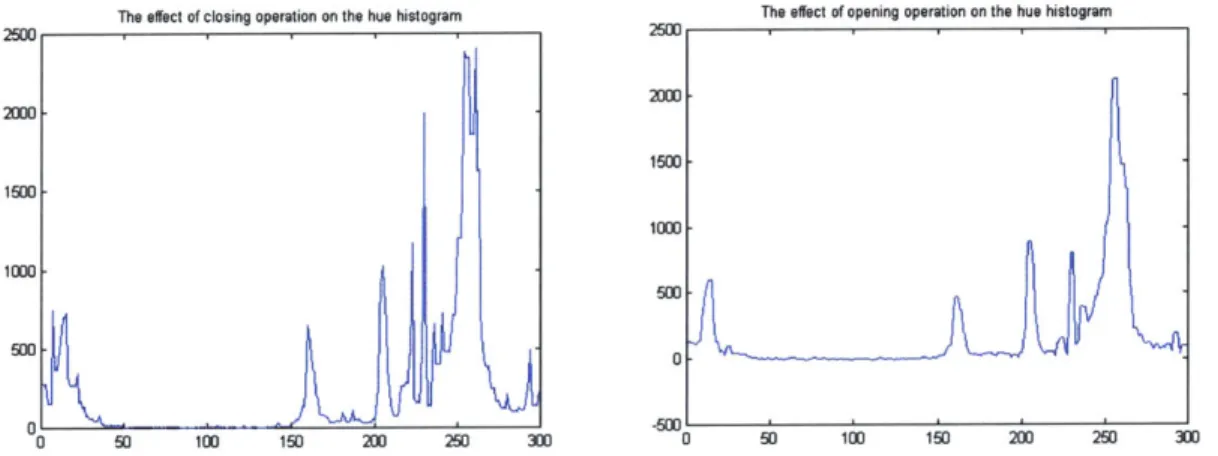
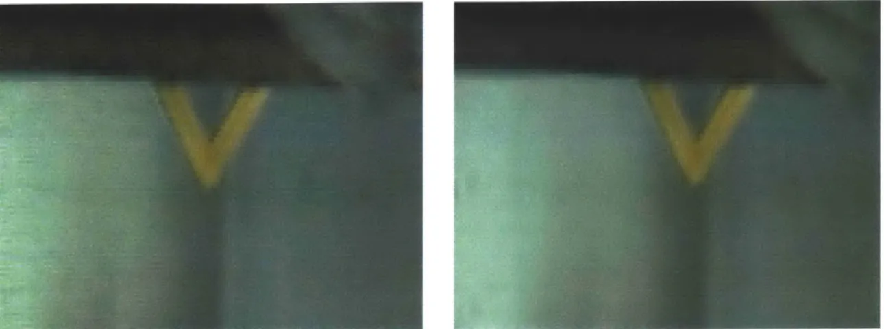
According to all segmentation techniques explained in the last section, so far no report of the segmentation techniques is confirmed to be the best approach. In our opinion, the region-based segmentation seems to give the best results in the sense of their feature selection, region base, instead of using edge or pixel information. However, typically the region-based segmentation required iteration process to achieve good results. For the feature-selection comparison purpose, the examples of edge detection, watershed algorithm [10] and histogram-based segmentation [29] are applied to the AFM images with poor and with good illumination conditions, the photograph of parrots and Lena, as shown in Figures 2.3, 2.4, 2.5 and 2.6 respectively. Before applying these segmentation algorithms, all of the original images are filtered with the edge-preserving filter, described later in section 4.3. All original images are shown in Figure 2.2. The edge detection is done using the canny operator in Matlab and the watershed algorithm based on the Gauch's algorithm is implemented using the gaussian filter with G=20 in

C++ language. The Matlab's command of the edge detection operation used in these

examples is "edge(I,'canny')", where I is a gray-scale image. The histogram-based

(a) (b) (c) (d)

Figure 2.2: (a) An original AFM image with poor lighting condition; (b) An original AFM image with good lighting condition; (c) An original parrots image; (d) An original Lena image.

-t-(a) (b)

Figure 2.3: (a) The canny edge detection; (b) Watershed segmentation; (c) Histogram-based segmentation.

(a) (b) (c)

Figure 2.4: (a) The canny edge detection; (b) Watershed segmentation; (c) Histogram-based segmentation.

(a) (b) (c)

Figure 2.5: (a) The canny edge detection; (b) Watershed segmentation; (c) Histogram-based segmentation.

. . .... .. ... ... -.... ... .....

(c)

(a) (b) (c)

Figure 2.6: (a) The canny edge detection; (b) Watershed segmentation; (c) Histogram-based segmentation.

segmentation, done in C++ language, uses our histogram valley-seeking technique, described later in section 4.4, to separate the intensity histogram of each picture into certain intervals. The computational time of the canny edge detection, watershed algorithm and histogram-based segmentation are in the order of less than 10 seconds, 2 minutes and less than 10 seconds respectively.

From the above results, the canny edge detection gives very poor performance, since usually the edges are not connected across the regions that have low value of gradient. Besides that there are some cases that two edges corresponding to the same line are obtained. Hence, the close boundaries of objects are remarkably difficult to recover from the edges. On the other hand, with use of the watershed algorithm, close contours of objects are guaranteed, since the segmentation results are often small-segmented regions. Although, most segmented regions preserve all edge information due to their local minimum property, its main disadvantage is over-segmented. The histogram-based segmentation of intensity also results in closed contour and most of the boundaries of segmented regions are corresponded to the objects' edge. Nevertheless, the images' variations, especially illumination, lead this method to over-segmentation problems. Particular, the AFM image with poor illumination condition separated into many segmented areas due to the shadow, illumination fading and noise effect. As a result of comparison above, the histogram-base segmentation is more suitable in several aspects: fast computational time, closed boundary and less over-segmentation of segmented

regions. Thus, this technique is then used as the coarse segmentation of the proposed algorithm, described later in chapter 4.

2.5: Clustering

In this section, several clustering techniques are briefly introduced along with their benefits and drawbacks as a background for the proposed clustering method in chapter 4. One of the well-known unsupervised classification methods that do not requires an assist of training sets is the clustering technique. Most clustering methods do not require any prior information of the sample data; therefore, certain characteristic in those data must be used to separate them into distinct groups or classes. The particular characteristic for defining the clustering is the most significant and basic issue that is

predetermined to satisfy the desired objective.

In the literature, the clustering algorithm is categorized into two main approaches:

the parametric approach and the nonparametric approach. Most parametric approaches

require a specific clustering criterion and a given number of samples so as to optimize the separation of samples according to that desired criterion. The class separability measures method is the best parametric approach. However, all parametric approaches demand iterative process to classify sampled points in specific spaces. In case of the image processing, these processes need to classify each pixel according to their criterion in each iteration. The convergence to satisfy that particular criterion is another problem of iterative procedure. Furthermore there is no discrete theory for determining the number of classes. The examples of the parametric clustering are the nearest mean reclassification algorithm, branch and bound procedure and maximum likelihood estimation (Fukunaga

[9]). For the nonparametric approach, the valleys of density function are used for

separation of each class. Nonetheless, the problem associates with this approach occurs when the shape of density functions becomes very complex to define the boundaries. The estimation of density gradient and reduced parzen classifier (Fukunaga [9]) and the three-dimensional clustering technique based on a binary three of RGB values (Rosenfeld [26]) are the examples of nonparametric procedures.

2.6: Summary

The image segmentation is the first component of the object recognition system, because the classification methods are based upon good segmentation results for solving the question of where each object does exist in the viewing image. Even though, various segmentation algorithms were proposed in last few years, the most common criterion of these algorithms is to partition the image into meaningful and uniform regions corresponding to the object presenting in the picture. All other general criteria are proposed and summarized by Haralick and Shapiro [14]. Several segmentation techniques, edge detection, watershed algorithm and histogram threshold are shown in this chapter for a feature-selection purpose. From the comparison, the histogram-base segmentation yields most suitable result in several aspects: fast computation, producing closed contour and less over-segmentation. Therefore, our proposed segmentation technique uses the histogram-base segmentation method as coarse segmentation. Then, the proposed clustering technique, described in chapter 4, refines this coarse segmentation to obtain better segmentation results.

Chapter 3: - Science of color

3.1: Introduction

In this chapter, we discuss a science of color that have been developed for standard measurements and representations by the "Commission International de l'Eclairage" (CIE). Most researchers have searched for the color representations that closely matches with human perception. This chapter covers the most important color representations, RGB, XYZ, YUV, YIQ and etc. The CIE recommended the well-known

CIELAB and CIELUV color spaces that closely represent human visualization. Both of

these color spaces are suitable for industrial-graphical applications. Our proposed algorithm, in chapter 4, also uses CIELUV color space as basic space for clustering. Lastly, the advantage and disadvantage of each color space are discussed.

3.2: Science of color

According to Isaac Newton's experiment, he discovered that a prism separates white light into strips of light or "visible spectrum". These strips of light, consisting of violet, blue, green, yellow, orange, and red, include all color in human visible range. Subsequently, these visible spectrums form white light by directing it through a second prism. This is the first evidence that spectral colors in the visible spectrum are the basic component of white light. Later on, light is discovered as a form of electromagnetic radiation that can be described by its physical property, wavelength (symbol X). Wavelength has units of nanometer (nm). The electromagnetic radiation varies from the shortest cosmic rays (10-6 nm) to radio waves with wavelength of several thousands meter. Therefore, the visible spectrum is a small range of electromagnetic spectrum from

380 to 780 nm.

Color science study can be divided into many topics such as radiometry, colorimetry, photometry, and color vision. It also covers how human beings distinguish color. However, this study is concentrate only on colorimetry, which numerically specifies color stimulus of human's color perception. Due to the recent development of

cheaper and more advanced image processing devices so that concepts and methods of colorimetry have become more practical.

The basis of colorimetry is developed by the "Commission Internationale de l'Eclairage" (CIE), well know as "CIE system". According to CIE, colorimetry is divided mainly into three areas: color specification, color difference and color appearance. In this study, we will focus on color difference and appearance. Most of the basis colorimetry theories have been developed by the CIE.

3.3: CIE system

There are a lot of existing color specification systems and color spaces; for example, RGB, XYZ, YIQ, LUV, however, the most significant of all color specification systems is developed by the CIE. A standard procedure for specifying a color stimulus within controlled viewing conditions was provided by the CIE system. It was first established in 1931 and further developed in 1964. Both of these systems are well known as the "CfIE 1931" and "CIE 1964" supplementary systems. Three important components of color perception are light, object and eye. These also were studied and standardized according to the CIE system as explained in following sections.

3.3.1: Light

All color perception came from lighting. A light source can be identified by

measuring its "spectral power distribution" (SPD - S(X)) using a spectroradiometer. This

SPD is defined in term of the relative distribution; so, the absolute SPD is not significant

for colorimetric formulation. There are many kinds of light sources. For example, daylight is the most common one, it is a mixture of direct and sky-scattered sunlight. Daylight's SPD varies from quite blue to quite red. In addition, artificial light sources are also widely used such as fluorescent, incandescent, and etc. The SPD variation of light sources is varies in wide range, therefore, it is not necessary to make color measurement using all possible light sources. The CIE suggested a set of standard illuminants in form

of a SPD-value table for industrial applications, but the illumination may not have a corresponding light source.

Moreover, the light source can be specified in term of "color temperature", which has unit of Kelvins, K. Color temperatures are separated mainly into three types, distribution temperature, color temperature and correlated color temperature. Firstly, a distribution temperature is temperature of a "Planckian" or black-body radiator. When the Planckian radiator, an ideal furnace, is kept at a particular temperature, it will discharge radiation of constant spectral composition. Secondly, a color temperature is the temperature of a Planckian radiator whose radiation has the same chromaticity as that of a given color stimulus. This is mainly used to prescribe a light source that has SPD similar to a Planckian radiator. Thirdly, a correlated color temperature is the temperature of a Planckian radiator whose color is match closely to a given color stimulus. This is commonly used for light source that has SPD quite different from a Planckian radiators such as fluorescent lamps.

According to CIE in 1931, three standard illuminants are known as A, B, and C which corresponding to the representation of incandescent light, direct sunlight, and average daylight respectively. Color temperature of A, B, and C are 2856, 4874 and 6774 K correspondingly and their SPD are shown in Figure 3.1. The CIE suggested a gas-filled tungsten filament lamp denoting the standard source A. The suggested standard sources B and C can be produced by using the standard source A combining with liquid color filters of specified chemical compositions and thickness. Later on, the CIE found that the illuminants B and C were unsatisfied for certain applications due to very small power in the ultraviolet region. Therefore, the CIE recommended another series of the D illuminants in 1964. The SPD of D65 also display in Figure and noticeably there is large distinction between illuminants of D65 and B or C around the blue-color wavelength. The most common used of D illuminants are D50 and D65 for the graphics arts and the surface color industries respectively.

A 1200 0900 B 600 .. 300 04 300 400 500 600 700 800 900 Wavelength ( nm )

Figure 3.1: Relatives SPDs of CIE standard illuminants: A, B, C and D65 (from "The Colour Image Processing Handbook" by S.J. Sangwine and R.E.N. Home [29]).

3.3.2: Object

Reflectance, R(X), of an object defines the objects' color as a function of wavelength. Reflectance can be described by the ratio of the light reflected from a sample to the light reflected from a reference white standard. Moreover, there are two types of reflectance, "specular" and "diffuse". Generally, some part of the light that direct into the surface will reflect back with the same angle as incident angle respect to the surfaces' normal axis, this is called specular reflection. Some part of the light will penetrate into the object. The rest will be absorbed and scattered back to the surface, this scattered light is called diffuse reflection. Measuring surface reflectance can be done using a spectrophotometer. The CIE also specifies standard methods to achieve instrumental precision and accuracy measurement. Firstly, a perfect reflecting diffuser is recommended as the reference white standard. Secondly, four different types of illuminating and viewing geometries, 45 degree/Normal, Normal/45 degree,

Diffuse/Normal, and Normal/Diffuse are recommended as shown in Figure 3.2. These four illuminating and viewing geometries can be divided into two categories: with and without an integrating sphere. Therefore, to obtain accurate reflectance result, it is very essential to specify the viewing geometry and illumination together with inclusion and exclusion of specular reflectance.

Illuminating Viewing

Integrating a Gloss trap

Viewing _sphere

Illuminating Baffle

0/45 d/O

Viewing Illuminating

Illuminating Integrating Gloss trap sphere

Viewing --- Baffle

45/0 0/d

Figure 3.2: Schematic diagram showing the four CIE standard illuminating and viewing geometries for reflectance measurement.

3.3.3: Eyes

The most important components of the CIE system is the color matching functions. These functions characterize how human eyes match color stimuli using a standard set of red, green, and blue references. Also, the color matching properties of the "CIE Standard Colorimetric Observers" are described by these functions.

The CIE color matching functions are based on the fundamentals of additive color mixing. In additive colorimetry, red, green and blue are the primary colors. For example, the addition of red and green light fluxes in appropriate proportions produces a new color, yellow. In general, a color "C" is produced by adding "R" units of the red primary,

"G" units of the green primary and "B" units of the blue primary. Thus, color match can

be formulated as the following equation:

C[C] = R[R] + G[G] + B[B]

Where R, G, and B are the amount of red [R], green [G], and blue [B] references stimuli required to match the C units of [C] target stimulus. The + and = sign represent an additive mixture and matching or defining respectively. Above equation is a unique

definition of the color C or known as Grassman's first law of color mixture. Another fundamental law of color mixture, Grassman's second law, defines a color as a mixture of two stimuli 1 and 2. It can be expressed by:

Stimulus 1 C1[C] = R1[R] + G1[G] + B1[B]

Stimulus 2 C2[C] = R2[R] + G2[G] + B2[B]

Resulting Color (C1+C2)[C] = (R1+R2)[R] + (G1+G2)[G] + (B1+B2)[B]

Generally, to represent a particular color required three independent quantities, red, green and blue primaries, so graphical representations have difficulty in representing a three-dimensional quantities onto two-three-dimensional plane. Thus, chromaticity coordinates, r, g, and b represent the proportions of red [R], green [G] and blue [B] instead of their absolute values become advantageous. Thus, only two of these variable are need for color representation. The chromaticity coordinates are calculated using:

r = R/(R+G+B)

g = G/(R+G+B)

b = B/(R+G+B)

Where r, g, and b are the proportions of the three reference basics, [R], [G], and [B], and r, g and b sum to unity. Color mixture is one of the significant property of a chromaticity diagram, For example, colors Cl and C2 are mixed additively, the resulting color C3 is on the straight line drawn from CI to C2.

According to the CIE in 1931, a set of standard color matching functions, known as the "CIE 1931 Standard Colorimetric Observer" (or 2 degree Observer) for use with visual color matching between 1-degree and 4-degree field sizes. These functions were derived from two equivalent sets of visual experiment carried out by "Wright"

(1928-1929) and Guild (1931) based upon 10 and 7 observers respectively. In order to combine

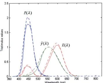
the results from these two sets of experimental data, they are normalized and averaged. The functions are denoted as r(X), g(X) and b(X) which corresponding to color stimuli of wavelengths 700 nm, 546.1 nm, and 435.8 nm for red, green, and blue primaries

respectively. Their units were adjusted to match an "equal energy white", which has a constant SPD over the spectrum. These functions are shown in Figure 3.3 below.

3, 2.5 2 1.5 0 -0.5 1 4 5 Wavelength (nm)

Figure 3.3: The color matching functions for the CfIE 1931 Standard Colorimetric Observer expressed using R, G, and B basic at 700, 546.1 and 435.8 nm, respectively.

From the plot, negative tristimulus value show that the light was added to the test color instead of to the red, green, and blue mixture. Consequently, these CIE 1931 2-degree color matching functions seriously underestimates sensitivity at wavelengths below 460 nm or at short wavelengths. Therefore, these functions, r(X), g(X) and b(X), were

linearly transformed to a new set of functions, x(X), y(X) and z(X), to get rid of the negative coefficients in the previous set. The x(X), y(X) and z(X) functions are also plotted on Figure 3.4. Furthermore, in 1964, a new set of color matching functions were formulated by the CIE for use with a more accurate correlation with visual color matching of fields of larger than 4 degree at the eye of the observer. This set of new functions was also derived from the experimental results by Stiles and Burch in 1959 and

by Speranskaya in 1959. These functions is called the "CIE 1964 Supplementary

Standard Colorimetric Observer" (or 10 degree Observer), and is denoted by xio(X),

yio(X) and z1o(X). These functions are also plotted on the same Figure 3.4 below.

2.5111 1 1 2 0.5 -05 0 - -- -- - .. 4.._ - --- '--350 400 450 50 550 6 650 70 750 WO Wavelength (nm)

Figure 3.4: The color matching function for the 1931 Standard Colorimetric Observer (solid lines) and for the 1964 Supplementary Standard Colorimetric Observer (dashed lines).

3.3.4: Tristimulus values

In the previous section, three essential components of color perception have been expressed in terms of functions of the visible spectrum. The standard colorimetric observer is defined by either the functions of x(X), y(X)and z(X) or the function of xio(X), ylo(X) and zio(X), to represent the person having normal color vision. The illuminants are standardized in terms of the SPD, S(X). In addition, the CIE standardized the illuminants and viewing conditions for measuring a reflecting surface. Surface reflectance is defined by R(X). Thus, the "tristimulus values", (X,Y,Z) are the triple numbers that described any color. These X, Y, and Z values define a color in the amounts of red, green and blue CIE basics required to match with a color by the standard observer under a certain CIE illuminant. So, these values are the integration of the products of S(X), R(X), and x(X), y(X) and z(X) in three components over the visible spectrum.

X = kJS(X)R(X) x(X) d% Y = kfS(X)R(X) y(X) d%

Where the k constant was chosen such that Y = 100 for the perfect reflecting diffuser.

And either ( x, y, z ) or ( x10, yio, Z10 ) can be use for small and large angle observer respectively.

For measuring self-luminous colors such as light-emitting colors or light sources, the following equation must be applied instead of the above equations, since the object and illuminant are not defined.

X = kIP(X) x(X) d

Y = kIP(X) y(X) d

Z = kfP(X) z(X) dX

Where P(X) is the function representing the spectral radiance or spectral irradiance of the source. Similarly to previous equations, the k constant is chosen such that Y = 100 for the

appropriate reference white. Usually, the areas color display have quite small angular subtense so that the CIE 1931 Standard Colorimetric Observer (x,y,z) is more accurate functions to be applied.

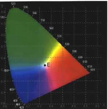
The color described in the CIE system generally plots on the "chromaticity diagram" shown in Figure 3.5 below. And the chromaticity coordinates are calculated using the formulation as followed.

x = X / (X+Y+Z)

y = Y / (X+Y+Z)

z = Z / (X+Y+Z) and x+y+z=1

Thus, only two variables from x, y and z coordinates are need to represent the color on the chromaticity diagram.

Figure 3.5: The CIE chromaticity diagrams for the 1931 2-degree standard colorimetric observer.

Noticeably, the region of all perceptible color is bounded by the horseshoe-shaped curve of pure monochromatic spectral colors or "spectrum locus", with a straight line connecting the chromaticity of extreme red and blue. This line is known as the "purple line". Point E in the middle of the spectrum locus is denoted the white color and other colors become more saturated toward the outer curve. An important feature of this chromaticity diagram is that only point, that lies on any straight lines, comes from an additive mixture of two color lights, that lies on the same straight line. This property is similar to the property in r, g and b coordinates. For example, if the amounts of two given colors are known, the position of the mixture of these two can be calculated.

Consequently, color specification can be specified by tristimulus values and chromaticity coordinates. Nevertheless, these representations cannot characterize color appearance, such as, lightness, saturation, and hue, it is very conceptual to visualize color from either tristimulus values or chromaticity coordinates. From tristimulus value, lightness or intensity can be calculated from Y value. The brighter the color is, the larger Y value will be. So, the CIE recommended another variables, "dominant wavelength" and "excitation purity" to represent the hue and saturation attributes respectively. These

two parameters can be calculated from chromaticity diagram as the following example, which specified attribute values plotted on Figure 3.6 below. Let a surface color, denoted

by point C, it observes with a particular illuminant, denoted by point N, on diagram

below. Draw a straight line from point N pass through point C to intersect with the spectrum locus at point D, so a dominant wavelength of color C is about 485 nm, which is equivalent to a greenish blue color. Also, excitation purity, (Pe), is a ratio of line NC to line ND. The excitation purity is closely related to saturation attribute. In this example, it is about 0.7, representing a quite saturation color.

Moreover, for a certain color that lie close to the purple line, like the color C', a line NC' doesn't join the spectral locus. The line NC' must be extended in the opposite direction until it intersect the spectrum locus. The intersection point on the spectrum locus denotes the "complementary wavelength", in this case is about 516 nm. Also, its excitation purity, which is about 0.85, is still a ratio of line NC' to line ND'.

Figure 3.6: Variable values plotted on the CiIE 1931 chromaticity diagram to demonstrate the calculation of the dominant wavelength, complementary wavelength and excitation purity. (from -"The Colour Image Processing Handbook" by S.J. Sangwine and R.E.N. Home [29]).

3.4: Uniform Color spaces and color difference formulas

To standardize color in industrial applications, the CIE proposed a way to

represent the color under a standard viewing conditions as described in previous section. Colorimetry is also useful for evaluating color difference in color quality control. However, after 1964, several color discrimination experimental results had shown that the XYZ space in chromaticity diagram from CIE 1931 and 1964 shown very poor uniformity results. Since, for all color, color differences are not represented by lines or circles of equal size from the white point E in Figure 3.5. The lines representing noticeable vary in size by about 40 to 1, being shortest in the violet region and longest in the green region on 1931 chromaticity diagram. This showed that attempt have been made to find a diagram that approaches more nearly "uniform chromaticity diagram". In

1937, MacAdam suggested the transformation below from (x,y) coordinate to (u,v)

coordinate and was accepted by the CIE in 1964.

u=4x /(-2x+ 12y+3) v=6y/(-2x +12y+3)

This transformation has been used until 1974, when more recent investigations, particularly from Eastwood, suggested that the v coordinate should increase by 50%, while the u coordinate remain unchanged. Then, in 1976, the CIE restrain this modification as a new chromaticity diagram called the "CIE 1976 uniform color space diagram" or " the "CIE 1976 UCS diagram, which represent uniform space perceptually. This new space, (u',v') coordinates, is a projective transformation from the tristimulus values or (x,y) coordinates as the following equations:

u' = 4X / (X + 15Y + 3Z)= 4x / (-2x + 12y + 3) v' = 9Y / (X + 15Y + 3Z)= 9y / (-2x + 12y + 3)

Unfortunately, this leads to an ambiguous decision from users' point of view to choose between (u,v) and (u',v') coordinates for more accurate color representation. Therefore,

this subject still continues to be under active consideration by the CIE colorimetry committee. The CIE 1976 UCS diagram, shown in Figure 3.7 below, also has the additive mixture property as well as the CIE 1931 and 1964 diagrams.

Figure 3.7: The CIE u'v' chromaticity diagram.

CIELAB and CIELUV color spaces

In 1976, the CIE recommended two new uniform color spaces, CIE L*a*b* (CIELAB) and CIE L*u*v* (CIELUV). CIELAB is a nonlinear transform of the tristimulus space to simplify the original ANLAB formulation by Adams in 1942, widely used in color industrial. CIELAB and CIELUV is given as the following equations:

3.4.1: CIELAB color space

L*=ll6f(- -16

a*=500[f( -f

b* =200

f-= O[f (YY

f (Zj]

And _{x 1/3}

if x >0.008856

f(x)=

Where X, Y, Z and Xo, Yo, Zo are the tristimulus values of the sample and a specific reference white respectively. Generally, the value of Xo, Yo, Zo can be obtained from the perfect diffuser illuminated by a CIE illuminant or a light source. L* denotes the lightness value and it is orthogonal to a* and b* spaces, while a* and b* represent relative redness-greenness, yellowness-blueness respectively. Converting from a*, b* axes to polar coordinate related to hue and chroma attributes as the following.

hab* tan-,lb

(a*

Cab*= a* 2 +b*2

The equation of color difference between two sets of L*a*b* coordinates (L*i,a*i,b*i)

and (L*2,a*2,b*2) is :

AEab = 2 +A*2+ *2

where AL* = L*2 - L*1, Aa* = a*2 - a*i and Ab* = b*2 - b*1.

or ab A*2 +AC *ab2 + *ab 2

where Al *ab = PV2(C *ab,1

C

b*

= {I- if a*, b*2 >a*2 _b*1

P _otherwise

and subscripts 1 and 2 represent the considered standard pair and considered sample pair respectively.

3.4.2: CIELUV color space

In CIELUV color space, L* is the same as in CIELAB color space. The other coordinate are given as the following:

U*= 13L *(u - uo)

V* = 13L * (v - vo)

h =

tan-C.. =

u*

_+v

*

Where u, v, Y and uO, vo, Yo are the u, v coordinates of samples and a suitable chosen white respectively. Variables, u and v in above equation can be substituted by either u

and v or u' and v'.

The equation of color difference is:

AEU = VAL *2 _{+Au *}2 _{+Av *}2

where AL* = L*2 - L*i, Au* = u*2 - u*I and Av* = v*2 - v*i.

or AE AL *2 +AC* 2+AH * 2

where AH * = pJ2(C *uvl

C

=-1 ifu*₁v*₂ >u*₂v*I

P

Iotherwise

and similarly subscripts 1 and 2 represent the considered standard pair and considered sample pair respectively.

Also, the saturation attribute can be calculated from CIELUV color space as followed:

The three dimensional representation of the CIELAB color space is shown in Figure 3.8 in L*a*b* coordinates. The value of L* vary from 0 to 100 corresponding to a black and reference white respectively. And a* and b* values represent the redness-greenness and yellowness-blueness values correspondingly. In CIELUV color space, u* and v* have the similar representation as a* and b*. The Cab* scale is an open scale on

horizontal plane with zero at the origin on the L* vertical line. The hue angle has range between 0 to 360 degrees; however, a pure red, yellow, green and blue colors are not located at 0 degree, 90 degree, 180 degree and 270 degree angles. Instead, hue angle is corresponding to the rainbow-color sequence.

L* 100 White _Yellow+) C*ab Green ()1 Red (+) Blue() 0 Black

Figure 3.8: A three dimensional representation of the CIELAB color space.

3.5: Different color space for representing color image

Generally, color space or coordinate system usually describes in three dimensions depending upon image processing application. Certain color space and color transformation is more suitable for one image processing system than regular RGB. This is discussed and explained in the following section. However, each color can be presented in one of these three-dimensional spaces. Different color spaces were derived

3.5.1: RGB color space

RGB color space is the most basic space for other types of color space in image processing. Also, RGB is the most commonly used one for both direct input and output signals in color graphics and displays. However, different devices provide variation in RGB outputs signals, so certain characteristic for each device must be taken into account during processing. Generally, most TV system uses either standard PAL/RGB or

NTSC/RGB in encoder and decoder operations. The RGB color gamut can be model as a

cube in Figure 3.9 below such that a point either on a surface or inside of this cube designates each RGB color. Then, the gray color can be describe on the main diagonal of this cube from black color, which has R, G and B values equal to 0, to white color, which has R, G and B values equal to maximum value of the cube.

B

Blue (O,OBmax) _{Cyan (0,Gmax,Bmax)}

Magent

(Rmax,O,Bma ) White (Rbaax,Gmax,Bmax) Gray color

Line

Green (0,Gmax,0)

~ G

Black (0,0,C)

Red (Rmax,0,0) Yellow (Rmax,Grnax,0)

R

Figure 3.9: RGB color space for representing each color.

The main disadvantage of RGB color space in most applications involves in natural high correlation between its elements: about 0.78 for R-B, 0.98 for R-G and 0.94 for G-B elements. Their components' unorthogonality is the reason why RGB color space is not desirable for compression purpose. Furthermore, other drawbacks of RGB color space are hard for visualization of color based on R, G and B components and its non-uniformity in evaluating the perceptual difference depending upon distance in RGB color

gamut. As mentioned in section 3.3.3 that normalization is required to transform from R,

G and B to r, g and b coordinate for illumination independence. According to some

experiments by Ailisto and Piironen in 1987 and Berry in 1987 verified that rgb coordinates are much more stable with changes in illumination level than RGB coordinates. Importantly, dark color pixels can produce incorrect rgb values because of noise effect, so that these pixels should be ignored in image segmentation process (Gunzinger, Mathis and Guggenbuehl, 1990). This dark color effect appears in the AFM image with poor illumination condition; thus, the noise level is very high as shown in section 4.6.

3.5.2: XYZ color space

As described in section 3.3.3, the XYZ color space was accepted by the CIE in

1931 and its main objective was to eliminate negative tristimulus values in each r, g and b

coordinate. The transformation from RGB to XYZ color space is described as the following equations given by Wyszecki and Stiles in 1982:

X = 0.490 R + 0.310 G + 0.200 B Y = 0.177 R + 0.812 G + 0.011 B

Z = 0.000 R + 0.010 G + 0.990 B

For the chromaticity coordinate system, the XYZ coordinate also has the normalized transformation equations given by Wyszecki and Stiles in 1982, similar to RGB coordinate. Thus, only two variables are independent and need to describe color in two-dimensional plane. The Y element in this color space represents the image illumination.

x = X / (X + Y + Z)

y = Y / (X + Y + Z)

From above transformation, reference stimuli in the CIE RGB space, R, G, B and white reference, convert into the following values:

Reference Stimuli x y

Reference Red 0.735 0.265

Reference Green 0.274 0.717

Reference Blue 0.167 0.009

Reference White 0.333 0.333

There are another two versions for transforming from RGB to XYZ color space, they are called EBU RGB (European Broadcasting Union) and FCC RGB (Federal Communications Commission, USA). Both of these transformations, based on the tristimulus values of cathode ray tube phosphors, have been employed in color reproduction of most color cameras. The transformation from RGB to EBU color space is given as the following:

X = 0.430 R + 0.342 G + 0.178 B

Y = 0.222 R + 0.707 G + 0.071 B Z = 0.020 R + 0.130 G + 0.939 B

And the transformation from RGB to FCC color space is given as the following:

X = 0.607 R + 0.174 G + 0.200 B

Y = 0.299 R + 0.587 G + 0.114 B Z = 0.000 R + 0.066 G + 1.116 B

According to, both transformations, reference stimuli in EBU and FCC color space, R, G, B and white reference, are calculate as the following values: