HAL Id: ensl-00274849
https://hal-ens-lyon.archives-ouvertes.fr/ensl-00274849
Preprint submitted on 21 Apr 2008
HAL is a multi-disciplinary open access archive for the deposit and dissemination of sci-entific research documents, whether they are pub-lished or not. The documents may come from teaching and research institutions in France or abroad, or from public or private research centers.
L’archive ouverte pluridisciplinaire HAL, est destinée au dépôt et à la diffusion de documents scientifiques de niveau recherche, publiés ou non, émanant des établissements d’enseignement et de recherche français ou étrangers, des laboratoires publics ou privés.
Revisiting and testing stationarity
Patrick Flandrin, Pierre Borgnat
To cite this version:
Revisiting and testing stationarity
Patrick Flandrin & Pierre Borgnat
Universit´e de Lyon, ´Ecole Normale Sup´erieure de Lyon, Laboratoire de Physique (UMR 5672 CNRS), 46 all´ee d’Italie, 69364 Lyon Cedex 07, France
E-mail: {FirstName.LastName}@ens-lyon.fr
Abstract. The concept of stationarity is revisited from an operational perspective that explicitly takes into account the observation scale. A general framework is described for testing such a relative stationarity via the introduction of stationarized surrogate data.
1. Introduction
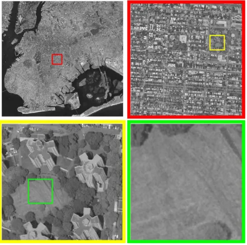
The concept of stationarity is ubiquitous in the signal and image processing literature, but its actual theoretical definition fails to be operational when confronted to practice. Strictly speaking, stationarity is a stochastic concept and—even when restricted to second order—its definition relies on an invariance with respect to any shift (in time or space), no matter how large this shift may be. This obviously contrasts with common practice which often accepts to loosely extend the definition to deterministic periodicities and to implicitly restrict its application to some finite observation range. As a result, practical “stationarity” turns out to be a relative concept, the very same physical object having the ability of appearing as stationary or not, depending on the observation scale. A schematic example of this situation is given in Fig. 1, in which zooming in on a scene makes successively appear, in an intertwined way, “stationary” and “nonstationary” features.1
2. A general framework
In order to cope with the aforementioned issues, a methodology has recently been proposed [8, 9], that basically relies on two ingredients:
(i) selecting an appropriate representation space in which local features can be compared to global ones so as to assess variability;
(ii) giving this assessment a statistical significance by comparing the actual observation with stationarized data sharing the same global structure.
2.1. A time-frequency/space-scale approach
Considered from either a stochastic or a deterministic point of view, stationarity of a time series is usually meant for an invariance of spectral properties over time. This naturally makes of the time-frequency plane [3] a natural representation space, with stationarity defined as an equivalence between local spectra and the global spectrum obtained by marginalization (see, e.g., [4, 5] for early attempts in this direction). Whereas the initial setting was developed for 1 The images used in Figs. 1 to 3 of this paper have been downloaded from http://maps.google.com/.
Figure 1. Zooming in on a given scene makes appear structures that, depending on the corresponding observation scale, can be interpreted as “stationary” or “nonstationary”. In this example, observation at a large scale (top left) evidences large distinct regions that make the overall scene “nonstationary”. At some smaller scale (top right), the scene is dominated by roughly periodic structures that turn it into a “stationary” one. Zooming in further (bottom left) turns back to “nonstationarity” whereas an observation at an even smaller scale (bottom right) reveals again a “stationary” structure attached to an homogeneous texture.
1D time series only, with spectra considered the usual way as a function of frequency (via the Fourier transform), it is clear that the proposed picture extends trivially to scale-based spectra (via the wavelet transform) as well as to 2D data in space. In any case, the rationale is to test for the variablity of differences (in a sense to be precised further) between local and global features over a given observation domain.
2.2. Stationarization via surrogates
From a practical point of view, local frequency/scale features will always exhibit fluctuations, and the question is to give them some statistical significance. For this to make sense, there is a need for some reference for the null hypothesis of stationarity. Since, in general, such a reference is not available, it is proposed to create it in a data-driven way by synthesizing a set of surrogate data that all share with the actual one the same global structure while being stationarized. For a given marginal spectrum, “nonstationary” processes differ from “stationary” ones by some organized structure in time or space. Recognizing that such an organization is encoded in
the spectrum phase, stationarized surrogates can then be easily constructed by randomizing uniformly the phase of the actual data spectrum while keeping its magnitude unchanged (this is in fact a new way of using the technique of surrogate data that has been primarily introduced in the physics literature and mostly used for testing nonlinearity [6]).
3. Tests
Within the above general framework, the principle of any surrogates-based test is therefore very simple, since it essentially amounts to
(i) creating a suitable set of stationarized surrogates from the observed data under test; (ii) elaborating from this set a statistical characterization of what the distribution of natural
fluctuations is supposed to be in the corresponding stationary situation;
(iii) computing the actual fluctuation for the observed data and deciding whether it is an outlier or not with respect to this distribution.
3.1. The 1D case
Two variations have been proposed in the 1D case, both based on (multitaper) spectrograms. In the first one [8], local and global frequency spectra are compared via a suitable “distance” combining the Kullback-Leibler divergence and the log-spectral deviation [7]. The mean-square deviation in time (over the considered interval) of this dissimilarity measure has been shown to follow a Gamma distribution. For a given confidence level, this modelling allows for the determination of an objective threshold on the basis of the two Gamma parameters, as estimated (e.g., in a maximum likelihood sense) from a limited number of surrogates (typically, about 50) [8]. (Matlab routines are available at http://perso.ens-lyon.fr/patrick.flandrin/stat test.html.)
A second variation [9] is aimed at by-passing the pre-requisite of the null hypothesis distribution modelling by directly considering the family of surrogates as a learning set. This viewpoint makes possible the use of (kernel-based) machine learning methods, and in particular of one-class support vector machines [10]. For the sake of learning, different time-frequency features can be envisioned but, as previously, nonstationarity is assessed by the fact that the actual data feature vector lies outside the domain of the empirical distribution derived from the training.
3.2. Some 2D extensions
Going from 1D to 2D can be made in a straightforward manner, replacing mutatis mutandis time by space and spectrograms by scalograms (i.e., squared magnitude of wavelet transforms). An example—in the spirit of the distance-based approach—is given in Figs. 2 and 3: it makes use of an undecimated dyadic wavelet transform, the overall test being constructed as the ℓ1-norm of a distance map computed pointwise. In order to compensate for the estimation variability, the wavelet transform is dyadically weighted in scale and, for both the distance map and its fluctuations, the comparison “local vs. global” is achieved in a directional way, ending up in fact with 3 different test measures attached to the horizontal, vertical and “diagonal” features extracted by the (tensor) 2D wavelet transform.
One further example is given in Fig. 4, dealing with a 2D fractional Brownian motion (fBm) with Hurst exponent H = 0.3. From a strictly theoretical point of view [1], such a self-similar process is classically referred to as nonstationary whereas, within the framework considered here, it appears as “stationary”. This result is however in accordance with the principles underlying the approach proposed here, since identifying “stationarity” with a statistical equivalence between local and global properties tends naturally to label as stationary those fractal processes (such as fBm) for which “the part is identical to the whole”. Moreover, the distance measure
original image
one surrogate image
distance map (H) average map (R = 50) 0 5 10 15 20 25 30 35 H V D test (p = 1)
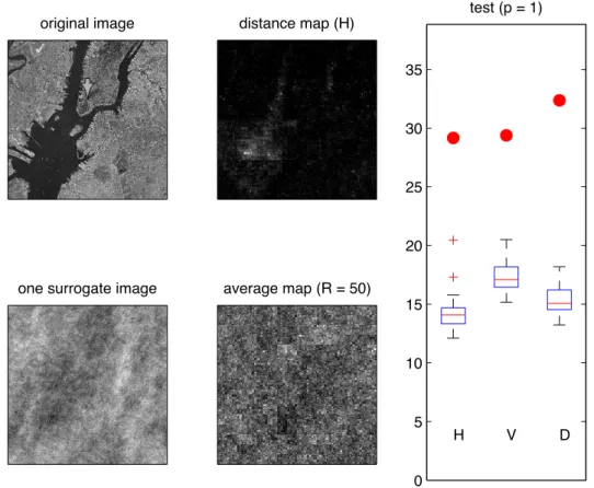
Figure 2. A “nonstationary” scene and one of its stationarized surrogates are displayed in the left column, while the middle column represents the corresponding (horizontal) distance maps between local and global scalogram spectra, the bottom one being an average based the use of 50 surrogates. The “nonstationary” nature of the scene at the considered scale is assessed in the far right diagram by the 3 test values (in horizontal (H), vertical (V) and “diagonal” (D) directions) for the actual scene (red dots) that appear as outliers when compared to the distributions boxplots of the corresponding surrogates test values.
aimed at quantifying the difference local vs. global is based on detail wavelet coefficients only, getting rid of the companion approximation coefficients that are known to carry the nonstationary part of processes with stationary increments [2]. Revisiting stationarity this way appears therefore as operational, adding a quantitative characterization to a meaningful interpretation.
4. Conclusion
A general methodology has been proposed for testing stationarity in an operational way, i.e., in a relative sense that explicitly includes the observation scale, and with a statistical significance stemming from the construction of an adequate set of surrogate data. Only the principle has been outlined, and the efficiency of the approach has been supported by simple, schematic examples. Whereas more details can be found in [8, 9], further studies are necessary to thoroughly evaluate performance and to make comparisons with related approaches.
original image
one surrogate image
distance map (H) average map (R = 50) 0 5 10 15 20 25 30 H V D test (p = 1)
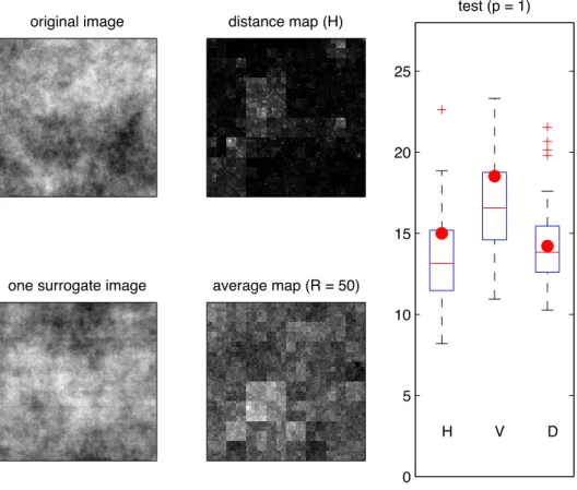
Figure 3. Same as in Fig. 2 when zooming in on a “stationary” region. At such a refined scale, stationarity is assessed by the test values for the actual scene (red dots) that lie within the corresponding distributions of the surrogates test values.
Acknowledgments
Part of this work is supported by ANR-07-BLAN-0191-01 StaRAC and conducted in collaboration with Pierre-Olivier Amblard (GIPSA-lab, Grenoble), C´edric Richard (UTT, Troyes) and Jun Xiao (ENS Lyon and ECNU, Shanghai).
References
[1] P. Embrechts and S. Maejima, Self-Similar Processes, Princeton Univ. Press, 2002.
[2] P. Flandrin, “Wavelet analysis and synthesis of fractional Brownian motion,” IEEE Trans. on Info. Theory, Vol. IT-38, No. 2, pp. 910–917, 1992.
[3] P. Flandrin, Time-Frequency/Time-Scale Analysis. San Diego: Academic Press, 1999.
[4] W. Martin, “Measuring the degree of non-stationarity by using the Wigner-Ville spectrum,” in Proc. IEEE ICASSP-84, pp. 41B.3.1–41B.3.4, San Diego (CA), 1984.
[5] W. Martin and P. Flandrin, “Detection of changes of signal structure by using the Wigner-Ville spectrum,”
Signal Proc., Vol. 8, pp. 215–233, 1985.
[6] J. Theiler, S. Eubank, A. Longtin, B. Galdrikian and J.D. Farmer, “Testing for nonlinearity in time series: the method of surrogate data,” Physica D, Vol. 58, No. 1–4, pp. 77–94, 1992.
[7] M. Basseville, “Distance measures for signal processing and pattern recognition,” Signal Proc., vol. 18, no.4, pp. 349-369, 1989.
original image
one surrogate image
distance map (H) average map (R = 50) 0 5 10 15 20 25 H V D test (p = 1)
Figure 4. Same as in Fig. 2, but in the case of a 2D fractional Brownian motion with Hurst exponent H = 0.3. Within the considered framework, such a self-similar process appears as stationary.
[8] J. Xiao, P. Borgnat and P. Flandrin, “Testing stationarity with time-frequency surrogates,” Proc.
EUSIPCO-07, Poznan (PL), 2007. Preprint available at http://prunel.ccsd.cnrs.fr/ensl-00175965/fr/.
[9] J. Xiao, P. Borgnat, P. Flandrin and C. Richard, “Testing stationarity with surrogates – A one-class SVM approach,” Proc. IEEE Stat. Sig. Proc. Workshop SSP-07, Madison (WI), 2007. Preprint available at http://prunel.ccsd.cnrs.fr/ensl-00175481/fr/.
[10] B. Sch¨olkopf and A.J. Smola, Learning With Kernels: Support Vector Machines, Regularization, Optimization