Combination of zero-valent iron and granular activated carbon for the treatment of groundwater contaminated with chlorinated solvents

Combination of Zero-Valent Iron and Granular Activated

Carbon for the Treatment of Groundwater Contaminated with

Chlorinated Solvents

by

Donald E. Tillman

Swiss Federal Institute of Technology, 1991

Submitted to the Department of Civil and Environmental Engineering In Partial Fulfillment of the Requirements for the Degree of

MASTER OF ENGINEERING in Civil and Environmental Engineering

at the

MASSACHUSETTS INSTITUTE OF TECHNOLOGY June 1996

O Donald E. Tillman. All rights reserved.

The author hereby grants to MIT permission to reproduce and to distribute publicly paper and electronic copies of this thesis document in whole and in part.

Signature of the Author

Department of Civil and Environmental Engineering May 17, 1996 Certified by

Philip M. Gschwend Professor of Civil and Environmental Engineering

Thesis Supervisor Accepted by

MASSACHUSETTS INST'ITU

OF TECHNOLOGY

JUN 0 5

1996

re Professor Joseph M. Sussman

Chairman, Departmental Committee on Graduate Studies

SARCMIVES

Combination of Zero-Valent Iron and Granular Activated Carbon for the Treatment of Groundwater Contaminated with Chlorinated Solvents

by

Donald E. Tillman

Submitted to the Department of Civil and Environmental Engineering May, 1996

In Partial Fulfillment of the Requirements for the Degree of Master of Engineering in Civil and Environmental Engineering

ABSTRACT

This study addressed the long-term economical benefits of adding the innovative zero-valent iron technology to a currently operating granular activated carbon (GAC) system. The concept is based on aboveground vessels, filled with zero-valent iron, which would pretreat the extracted water before it flows through the GAC. This was examined for the remediation of the CS-4 groundwater plume underlying the Massachusetts Military Reservation at Cape Cod. Contaminants to be treated are tetrachloroethylene, trichloroethylene, 1,2-dichloroethylene, 1,1,2,2-tetrachloroethane in concentrations up to 62 ppb. The study was based on data from literature and from reports of previous studies of the site. No laboratory tests were conducted.

The results indicated that the combination of these two technologies is pobably not an effective means to reduce long-term treatment costs. The investments of adding an aboveground zero-valent iron vessel do not balance the overall savings. The build up of vinyl chloride (VC) as a result of the degradation of the chlorinated hydrocarbons by the iron was a major concern and was modeled using kinetic expressions. It was shown that an increase of VC over regulatory limits must be expected if contact time of the contaminated water with the iron is more than 0.17 hr. Depending on the degradation rate of VC, a worst case increase up to 50 ppb was modeled. The design of the combined treatment system impeded excessive build up of VC. A required bulk volume of iron of 500 ft3 was estimated to pretreat the water. A bench-scale study should be conducted to verify the results.

Thesis Supervisor: Dr. Philip M. Gschwend

Acknowledgments

I would like to address sincere thanks to several people who supported me greatly in getting this thesis done, and who also provided an environment in which I could thoroughly enjoy my year at MIT. Especially I would like to mention:

Philip M. Gschwend as my thesis advisor for his generous giving of time, excellent

guidance, and patient explanations. His enthusiasm and "fire" for the scientific work always motivated and encouraged me enormously. He not only taught me how to critically review and question my own and other peoples work, but also made it possible that I could move from the first row in the classroom (and take notes) to the last one (and making some back of the envelope calculations).

Lynn W. Gelhar, who guided the whole team project process in a most superior and smooth way. His help and constructive inputs are greatly acknowledged.

Dave H. Marks and Shawn P. Morrisey, who showed me the way through the corridors

of MIT. Thanks for their function as a lighthouse, helping me directing my boat around the cliffs. I appreciated the always open doors, their humorous spirit and good advice. All the colleagues from the M.Eng. program, who helped creating and maintaining a pleasant working environment. In particular, I would like to thank my team-mates, Crist

Khachikian, Alberto Lizaro, Enrique L6pez-Calva, Christine Picazo, and Pete

Skiadas, who never lost their humor and happiness despite the many long working nights in the M.Eng. Room. Special thanks to Crist who always helped me climbing over small hills (e.g. Vermont) and big mountains (e.g. Switzerland).

My roommates Romana and Marko, with whom I greatly enjoyed sharing our apartment. Our common study breaks, discussions and jokes will not be forgotten. Thanks for Romanas famous cakes and cookies which prevented me from starving.

Most of all, I thank my Parents for the wonderful education and support I received throughout my live. They provided the foundation for my achievements.

Table of Contents

A bstract ... ... 2

A cknow ledgm ents... 3

List of Figures... ₆ List of Tables ... ... 7

1. Introduction ...

8...

2. Background and Site Description...

...

11

2.1 Location... 11

2.2 M M R Setting and History ... 12

2.3 Importance of Aquifer Restoration... 13

2.3.1 Natural Resources ... 13

2.3.2 Land and W ater Use ... ... 13

3. Current Situation ...

...

... 15

3.3 Existing Remedial Action... ... 19

3.3.1 Interim Remedial Action ... ... 19

3.3.2 Pumping Schemes and Treatment Technology ... 20

3.4 Objectives for Final Remedy... ... 20

3.4.1 Expected Performance of Pump-and-Treat: General Review ... 21

3.4.2 Conclusion... ... 23

4. Expected Performance of GAC

...

... 24

4. 1 Description of System ... 24

4.2 Theoretical Background ... ... ... ... ... 25

4.2.1 General Considerations ... 25

4.2.2 Preparation and Reactivation of the Carbon... ... 25

4.2.3 Adsorption Capacity... ... 26

4.2.4 M ulticomponent Solutions ... ... 27

4.2.5 Kinetics of Adsorption ... ... 29

4.3 Adsorption Capacity of GAC at CS-4 ... ... 30

4.3.1 Isotherms for Single Components ... ... 30

4.3.3 Loading Rate ... ... ... 32

4.3.4 D esign Loading Rates ... ... 36

4.3.5 Carbon Exchange Rate ... 37

4.4 Cost Estimation ... 37

5. Technology Review...

40

5.1 G A C E valuation ... ... 40

5.1.1 Evaluation Criteria for GAC Selection...40

5.1.2 Other Technologies Considered ... 40

5.2 Innovative Treatment Alternatives ... 42

6.

Abiotic

Dehalogenation with Zero-Valent Iron...43

6.1 Description of Technology ... ... ... 43

6.2 Degradation Process ... ... 44

6.2.1 Kinetic Considerations ... ... .... ... ... ... ... 46

6.2.2 H alf-life D ata... ... ... ... ... ... 48

6.3 Design Parameters ... ... 50

6.3.1 Required Degradation Time ... ... ... 50

6.3.2 Required Volume of Iron ... ... ... 57

6.3.3 Flowrate Through Iron ... .. ... ... 58

6.3.4 Effluent Concentrations... . ... .... .... ... 58

6.4 Cost... ... .... ... .... ...59

7. Combination of Zero-Valent Iron and GAC

...

61

8. Conclusions ...

64

R eferences ... .... ... ... ... 65

Appendices: Appendix A: Chemistry of Plumewater and Soil at Source ... 74

Appendix B: Literature Values for Freundlich Constants ... ... 76

Appendix C: Isotherms of Calgon Carbon Corporation ... ... 77

Appendix D: Empty Bed Contact Time (Calgon Carbon Corporation) ... 78

Appendix E: Spreadsheet Calculations for Carbon Exchange and Zero-Valent Iron Cost ... 80

List of Figures

Map of the Commonwealth of Massachusetts. ... 11

CS-4 plume and well-fence location ... ... 17

Source loadings for the CS-4 plume (Sum of PCE, TCE and DCE only)...19

GAC configuration at CS-4. ... 24

Expected concentrations versus time for scenario 1. ... 53

Sensitivity analysis of DCE with respect to half-life of DCE degradation....54

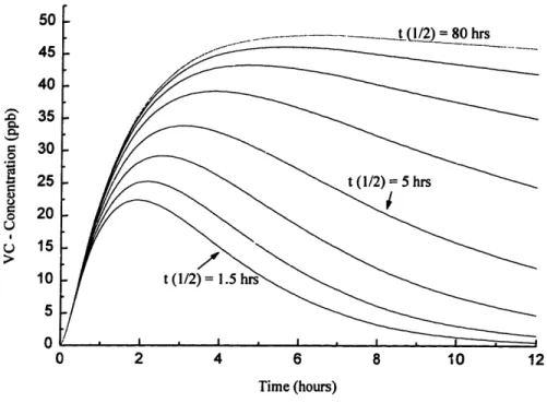
Sensitivity analysis of VC with respect to half-life of VC degradation...55

Expected concentrations versus time for scenario 2 ... 56

List of Tables

3-1: Groundwater properties (E. C. Jordan, 1990; LeBlanc et al., 1991;

A BB ES, 1992b)... 16

3-2: Contaminants of concern and treatment target levels... 18

4-1: Freundlich constants from Dobbs and Cohen, (1980) and Calgon Carbon Corporation (1996). Capacities are calculated for maximum contaminant concentrations encountered at CS-4 ... ... 30

4-2: Two scenarios for influent concentrations... 31

4-3: Inflow concentrations to treatment facility, scenarios 1 and 2 ... 32

4-4: Calculation of loading rates with different methods for scenario 1. ... 35

4-5: Calculation of design loading rates LR for the two scenarios ... 36

4-6: Carbon usage rate for two different scenarios of plume concentrations. ... 37

4-7: Total estimated carbon exchange cost (net present value) over expected duration of pum ping. ... ... ... ... 39

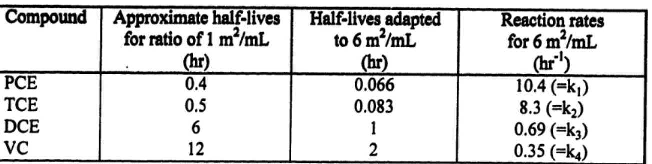
Table 6-1: Half-lives reported from different references (Gillham, 1996a). Normalized to the same area-to-volume of solution ratio of 1 m2/mL...48

Table 6-2: Half-lives for TCE from field measurements (Gillham, 1996a). ... 49

Table 6-3: Half-lives from column tests ... 49

Table 6-4: Design reaction rates. ... 52

Table 6-5: Design contact time ... 57

Table 6-6: Influent and effluent concentrations of iron vessel. ... 59

Table 7-1: Carbon exchange cost after zero-valent iron pretreatment ... 62

Table 7-2: Net savings yielding in combination of GAC with zero-valent iron ... 63 Ttible Table Table Table Table Table Table Table , Table 4

1. Introduction

1.1 Context

The Cape Cod aquifer is contaminated by various pollutants emanating from the Massachusetts Military Reservation (MMR). One such plume of contaminants, termed Chemical Spill 4 (CS-4), is being contained. At present, a pump-and-treat system has been installed as an interim remedial action to prevent the advancement of the plume. Contaminated water is extracted at the toe of the plume, treated to reduce the contaminant concentrations to regulatory levels, and discharged back into the aquifer. However, operation and maintenance costs of pump-and-treat systems are high. A final remedial plan must be formulated to completely clean up the groundwater.

To develop a final remediation scheme for the CS-4 site was the project objective of a team of six graduate students at the Massachusetts Institute of Technology (MIT). This team-project was completed within the frame of the Masters of Engineering Program of the Department of Civil and Environmental Engineering at MIT. Each team member addressed a different aspect of the overall objective in depth. The findings of these studies were then put together to present a possible, final remediation scheme. The executive summary and the results of the team-project are given in Appendix F.

Within this context and as part of the overall team-project, this thesis focuses on the aboveground treatment of the extracted groundwater.

1.2 Problem

At almost all remediation sites where contaminated groundwater is involved, the prevailing method to achieve cleanup goals is pump-and-treat. Treatment of the extracted groundwater is often achieved by a Granular Activated Carbon (GAC) system (Mackay and Cherry, 1989). This concept may also be considered as a final remedial system for the CS-4 site.

GAC is a proven and reliable technology (Stenzel et al., 1989). However, one of the disadvantages is that the operation and maintenance cost are relatively high. Principal cost contributions are due to the periodical exchange and reactivation of the exhausted carbon, when no more organic compounds can be adsorbed to it. Since typical pump-and-treat remediation requires operation of the system over a long period of time (see chapter 3.4.1; for CS-4 approximately 90 years), this procedure results in high long-term costs. More cost-effective treatment alternatives are needed.

1.3 Objectives

The objective of the present thesis was to answer to the following questions:

* Can the currently operating GAC system at the CS-4 site be optimized in a way which would result in less cost-intensive long-term operation?

* What are the expected savings for such an optimization?

This task was addressed by focusing on a concept of combining the currently operating GAC treatment with another treatment technology. Consequently, the first goal of this study was to get a thorough understanding of the principles, cost and design considerations of the GAC treatment technology. The second goal was to estimate potential cost savings by combining the GAC with an alternative treatment technology.

1.4 Scope

All the used data was based on the review of reports of previous studies at the CS-4 site as part of the Installation Restoration Program (IRP), and on the other theses within the CS-4 team-project. Also, literature data and direct information provided by treatment technology suppliers were consulted.

Chapter 2 and 3 describe briefly the site, its characteristics and the current remedial situation. This part was adapted primarily from the team-project.

Chapter 4, 5, and 6 elucidate the GAC treatment technology, treatment alternatives, and the emerging valent iron technology, respectively. The costs of GAC and zero-valent iron technology were only estimated to an extent which allows comparison of the technologies and estimation of savings or cost due to their combination. Specific evaluation of the construction and design considerations of the combination concept were not examined.

The combination concept was developed to a preliminary stage only. While conclusions regarding its feasibility can be drawn, greater details need to be studied further.

2. Background and Site Description

2.1 Location

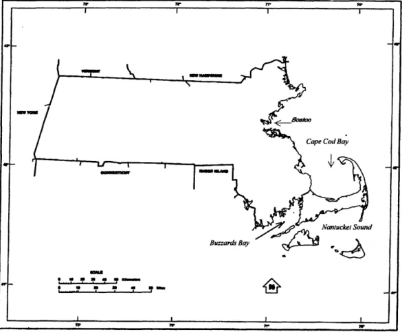
Cape Cod is located in southeastern of Massachusetts (Figure 2-1). It is surrounded by Cape Cod Bay on the north, Buzzards Bay on the west, Nantucket Sound to the south, and the Atlantic Ocean to the east. Cape Cod, a peninsula, is separated from the rest of Massachusetts by the man-made Cape Cod Canal.

Figure 2-1: Map of the Commonwealth of Massachusetts.

The MMR is situated in the northern part of western Cape Cod (Figure 2-2). Previously known as the Otis Air Force Base, the MMR occupies an area of approximately 22,000 acres (30 square miles).

Figure 2-2: Location of MMR.

2.2 MMR Setting and History

The MMR has been used for military purposes since 1911. From 1911 to 1935, the Massachusetts National Guard periodically camped, conducted maneuvers, and provided weapons training in the Shawme Crowell State Forest. In 1935, the Commonwealth of Massachusetts purchased the area and established permanent training facilities. Most of the activity at the MMR occurred after 1935, including operations by the U.S. Army, U.S. Navy, U.S. Air Force, U.S. Coast Guard, Massachusetts Army National Guard, Air National Guard, and the Veterans Administration.

The majority of the activities consisted of mechanized army training and maneuvers as well as military aircraft operations. These operations inevitably included the maintenance and support of military vehicles and aircraft as well. The level of activity varied greatly over the operational years. The onset of World War II and the demobilization period following the war (1940-1946) were the periods of most intensive army activity. The period from 1955 to 1973 saw the most intensive aircraft operations. Today, both army training and aircraft activity continue at the MMR, along with U.S. Coast Guard activities. However, the greatest potential for the release of contaminants into the

environment was between 1940 and 1973 (E.C. Jordan, 1989a). Wastes generated from these activities included oils, solvents, antifreeze, battery electrolytes, paint, waste fuels, metals and dielectric fluids from transformers and electrical equipment (E.C. Jordan,

1989b).

2.3 Importance ofAquifer Restoration

Cape Cod is characterized by its richness of natural resources. Ponds, rivers, wetlands and forests provide habitat to numerous species of flora and fauna. Many of the Cape's ponds and coastal streams serve as spawning and feeding grounds for a variety of fish (Massachusetts Executive Office of Environmental Affairs, 1994). The Crane Wildlife Management Area, located south of the MMR in western Cape Cod, is home to many species of birds and animals. In addition, throughout the Cape there are seven Areas of Critical Environmental Concern (ACEC) as defined by the Commonwealth of Massachusetts. These were established as areas of highly significant environmental resources and protected because of their central importance to the welfare, safety, and pleasure of all citizens.

2.3.2 Land and Water Use

The majority of the land in Cape Cod is covered by forests or is "open land". One quarter of the land is residential, and less than 1% of the land is used for agriculture or pasture (Cape Cod Commission, 1996).

Water covers over 4% of the surface area of Cape Cod. This water is distributed among wetlands, kettle hole ponds, cranberry bogs, and rivers. Nevertheless, all 15 communities of Cape Cod meet their public supply needs with groundwater. Falmouth is the only municipality that uses some surface water (from the Long Pond Reservoir) as a drinking water source. Approximately 75% of the Cape's residents use water supplied through public works, while the remaining use private wells within their property.

Agriculture constitutes a part of the water use in Cape Cod. Cranberry cultivation is an important part of the economy of the Cape and a water-intensive activity. The fishing industry also provides a boost to the Cape's economy. Tourism accounts for a substantial part of the Cape's economy, and therefore the surface water quality is important.

3. Current Situation

3.1 Site Characterization

Site characterization was based on previous studies in the area. Equilibrium sorption (since this factor may greatly affect the fate of the contaminants) however, was tested in the laboratory (Appendix F; Khachikian, 1996).

3.1.1 Hydrogeology

On a regional scale, the geology of western Cape Cod is composed of two glacial moraines deposited along the western and northern edges and a broad outwash plain between the two moraines. The outwash is composed of poorly sorted fine to coarse grained sands, and its thickness varies from approximately 175 ft to 325 ft. Precipitation

is the sole source of recharge to the aquifer. Values of recharge are between 18 in/yr and

23 in/yr. A value of 380 ft/day has been accepted as a representative value of average

hydraulic conductivity of the outwash sands (regional scale). Effective porosity is estimated to be about 0.39, and average hydraulic gradient is 0.0014 (Lazaro, 1996; L6pez-Calva, 1996).

The groundwater flow model, which was developed for the CS-4 area, showed great sensitivity to the properties of the glacial moraine. The calibrated model (based on head distributions and particle tracking) used an average hydraulic conductivity of 220 ft/day, a seepage velocity of 0.8 ft/day, and recharge of 19 in/yr (Appendix F; Laizaro, 1996; L6pez-Calva, 1996).

3.1.2 Retardation

The organic carbon content in the sediments is very low (in general, less than 0.01%). Because of this low organic content, the degree of sorption of the contaminants is relatively small. The retardation coefficients (R), are 1.04, 1.10 and 1.25 for DCE, TCE and PCE, respectively. For the more strongly sorbing PCE, the retarded longitudinal

macrodispersivity increases by a factor of 2.1. For the least sorptive compound (DCE), the velocity variances introduced by sorption are small as reflected by a small (factor of 1.2) increase in the longitudinal macrodispersivity (Appendix F; Khachikian, 1996). 3.1.3 Chemistry of Groundwater

In order to design treatment processes for the contaminated groundwater, a basic examination of the chemistry of the groundwater must be performed. The properties of the groundwater of particular interest are shown in Table 3-1. The groundwater contains high values of dissolved oxygen (5-10 mg/L) although the values vary with depth (depth

< 100 ft below water table). Values for pH range between 5 and 7, and the temperature is

approximately 100_{C. The range of concentrations of iron and manganese are also of}

particular interest since high concentrations can influence a treatment system considerably (precipitation, plugging) (E. C. Jordan, 1990; LeBlanc et al., 1991; ABB ES,

1992b).

Table 3-1: Groundwater properties (E. C. Jordan, 1990; LeBlanc et al., 1991; ABB ES, 1992b).

Propierty Value

Dissolved oxygen (mg/L) 5.0-10.0 Suspended solids low

pH 5-7

Iron (jpg/L) up to 3,500 (but normally very low)

Manganese (jig/L) up to 600

Temperature 130 C

3.2 Groundwater Plume

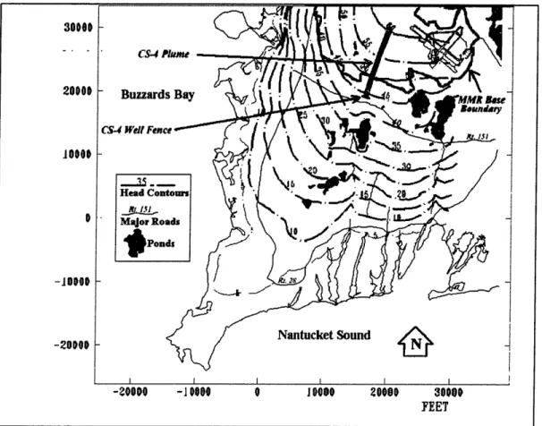
The CS-4 plume is located in the southern part of MMR as shown in Figure 3-1, moving southward. According to E. C. Jordan (1990), CS-4 is 11,000 ft long, 800 ft wide and 50

ft thick (5 ppb contour). These dimensions of the plume have been defined using field

observations. However, by using the developed contaminant transport model and simulating a continuous input of the contaminants, the plume resulting from the

simulations had greater dimensions than the plume defined by field observations. Average dimensions were 1,180 ft for the width, 60 ft for the height, and 14,660 ft for the length. However, this model was demonstrated to be sensitive to variations in input values of hydrogeologic parameters (Appendix F; L.zaro, 1996).

Figure 3-1: CS-4 plume and well-fence location.

3.2.2 Contamination

The results of the field sampling are shown in Appendix A (E. C. Jordan, 1990). Because soil contamination has been identified as the source of the groundwater contamination, the table in Appendix A lists not only the maximum concentrations of the chemicals which were found by sampling the aquifer downgradient of the source, but also the levels in the soil at the source location. In the mean time, the contaminated soil has been excavated and thus the source of the groundwater contamination removed.

A comparison of the measured values of each addressed compound with their regulatory limits (Maximum Contaminant Levels, MCL) show that four compounds exceed the MCL:

* Tetrachloroethene (PCE) * Trichloroethene (TCE)

* 1,2-Dichloroethene (DCE, total of cis- and trans isomer) * 1,1,2,2-Tetrachloroethane (TeCA)

These four compounds are therefore considered as contaminants of concern, which need to be removed from the groundwater. Table 3-2 summarizes the sampled concentrations. Maximum measured concentrations and average concentrations within the plume as well as an approximate frequency of detection and the individual regulatory limits are given. Average concentration values represent only an approximation, since their determination depends on a definition of the plume border.

Table 3-2: Contaminants of concern and treatment target levels.

Tetrachloroethylene 62 18 14/20 5

(PCE)

a No Federal of Massachusetts limits existent. Therefore, a risk-based treatment level was proposed. This was calculated assuming a lx10-5 risk level and using the US EPA risk guidance for human health exposure scenarios.

The total mass of the contaminants, which were discharged from the now removed contaminated soil to the aquifer (source loading), was calculated "backwards" from the concentrations found in the plume (Appendix F; Laizaro, 1996). Due to limitations in the

program code, PCE, TCE and DCE were simulated as one contaminant. Figure 3-2 shows that at least 290 kg (sum of columns) of the compounds of concern were discharged to the aquifer.

The source was modeled as a continuous source input. From groundwater velocity data, it was determined that the contamination must have started at least 15 years ago. The source loading was modeled as seven 5 year intervals (from 1960 to 1993, Figure 3-2).

Figure 3-2: Source loadings for the CS-4 plume (Sum of PCE, TCE and DCE only).

3.3 Existing Remedial Action

The currently operating remedial action was designed as an interim solution, with the objective to contain the plume against further migration. This is achieved by a pump-and-treat system, consisting of the following components:

* Extraction of the contaminated groundwater at the leading edge of the plume by 13 adjacent extraction wells, forming a well-fence as shown in Figure 3-1.

* Transport of the extracted water from the well-fence through pipe to the treatment facility, which is located at the edge of the MMR area.

* Treatment of the water with a Granular Activated Carbon (GAC) system.

* Discharge of the treated water back into the aquifer through an infiltration gallery, which is located next to the treatment facility.

I

At the time of the implementation of the interim system (1993), it was expected that it would operate about 5 years, until a final remedial system is chosen and implemented.

Since the treatment facility started operating in November 1993, the extracted water was predominantly clean. From time to time though, detected concentrations of the contaminants of concern in the water were up to 0.5 ppb (ABB ES, 1996).

3.3.2 Pumping Schemes and Treatment Technology

The treatment facility will not be addressed here but discussed in detail in Chapter 4. With regard to the pumping rates, the extraction pumps are currently operated at an overall pumping rate of 140 gpm. Simulations using the current well-fence indicated that this pumping rate is appropriate (Appendix F; L6pez-Calva, 1996). Therefore, for all further calculations in this report, an overall pumping rate of 140 gpm was used.

3.4 Objectives for Final Remedy

In contrast to the objective of the current interim remedial action, the final remedial action will address the overall, long-term objectives for the CS-4 Groundwater Operable Unit which are as follows (ABB ES, 1992b):

* Reduce the potential risk associated with ingestion of contaminated groundwater to acceptable levels.

* Protect uncontaminated groundwater and surface water for future use by minimizing the migration of contaminants.

* Reduce the time required for aquifer restoration.

In terms of treatment objectives, the target levels for the treatment of the water are defined through the established Maximum Contaminant Levels (MCL, Table 3-2).

The final remedial system could be chosen to be the same as the existing interim one, or could encompass other remedial concepts.

3.4.1 Expected Performance of Pump-and-Treat: General Review

Since the CS-4 pump-and-treat system was put into operation just recently (November 1993, performance data is lacking. In order to get an estimate of the expected performance, the performances of pump-and-treat systems at other locations were briefly studied by reviewing the literature. At almost all remediation sites, where contaminated groundwater is involved, the prevailing method to achieve cleanup goals is pump-and-treat (Mackay and Cherry, 1989). Specifically, this technology is employed at approximately three-quarters of the Superfund sites where groundwater is contaminated and at most sites governed by the Resource Conservation and Recovery Act (RCRA) (MacDonald and Kavanaugh, 1994).

Numerous authors have raised serious concerns about the ability of existing technology to restore contaminated groundwater to environmentally and health-based sound conditions (Mackay and Cherry, 1989; Doty and Travis, 1991; MacDonald and Kavanaugh, 1994). These and other researchers argue that one of the major disadvantages of pump-and-treat systems is the necessity of pumping over a long period of time. In the case of the CS-4 site, the groundwater transport model (retardation included) predicted continuous pumping for approximately 90 years for the removal of the contaminants from the aquifer (Appendix F). MacDonald and Kavanaugh (1994) however state that it is almost impossible to predict how long pumping and treating will take in order to restore an aquifer.

Other studies have shown that pump-and-treat, in conjunction with other treatment technologies, is able to restore aquifers effectively (Ahlfeld and Sawyer, 1990; Bartow and Davenport, 1995; Hoffman, 1993). However, both sides agree that pump-and-treat is an effective means of controlling the plume migration. Conclusively, the interim CS-4 pump-and-treat system is an appropriate way to quickly respond to the plume migration. According to a study of the National Research Council (NRC, 1994), groundwater restoration through pump-and-treat may be possible only for sites with relatively simple contamination scenarios. At more complex sites (e.g. most Superfund sites), health-based

drinking water standards may not be achieved. Although thousands of pump-and-treat systems are operating in the United States (the exact number is unknown), comprehensive studies of the performance of individual pump-and-treat systems are rare. In all, the NRC identified 77 sites where sufficient data was available to evaluate the performance of the system (MacDonald and Kavanaugh, 1994). At only 8 of the 77 sites, cleanup goals were reportedly achieved after one to several years of operation. The NRC committee attributed the success of cleanup in part to the relatively simple characteristics of the sites and the rapid initial response. The source of contaminants were quickly controlled and the plume of contaminated groundwater was therefore relatively small. At the other 69 sites, the pumping caused an initial decrease in contaminant concentrations in the extracted water, followed by a leveling of concentration and sometimes a gradual decline. Also, the characteristics of the contaminants play a major role. While for dissolved solutes or LNAPL's (Light Non-Aqueous Phase Liquids), some success in pumping a significant fraction to the surface has been reported, for DNAPL's, which are more dense than water, very little success has been achieved in even locating them in the subsurface, let alone removing them.

On the basis of the data from the 77 sites, the NRC committee concluded that cleaning up groundwater to health-based standards using conventional pump-and-treat systems may be feasible at a limited number of sites having relatively simple characteristics. The sites that are simplest to clean up are those where the contaminants are present in dissolved form, the geology is relatively homogenous, and the contamination is recent. However, the committee determined that portions of most sites will remain contaminated above health-based levels even after long-term pumping operation (MacDonald and Kavanaugh, 1994).

Applying these generalizations to the CS-4 situation, it was concluded that a pump-and-treat system will be able to contain the plume as an interim action, in order to finally remediate the aquifer, long duration of pumping must be expected. What appears

favorable to clean-up though is the very low organic matter content of the subsurface, which results in small retardation factors (Khachikian 1996; Appendix F).

3.4.2 Conclusion

The final remedial design of the CS-4 plume has to consider three options:

* Optimize the current pump-and-treat system: Number of extraction wells, pumping rates, flow rates through GAC, configuration of GAC.

* Enhance current pump-and-treat system by combining it with other treatment technology. For example, through the implementation of bioremediation, the concentration of contaminants in the groundwater may get attenuated and therefore the GAC would get loaded with less contaminants (saving in operation costs). Or, the GAC could be combined with another aboveground treatment process, which may result also in less operation cost for the GAC as well.

* Change the pump-and-treat scheme to an in situ scheme, for example implementation of bioremediation (Skiadas, 1996) or a reactive wall (Goo, 1996). This study focused on the second option. As it can be seen in chapter 6, the zero-valent iron technology was selected to be combined with the GAC.

In the following chapter 4, the GAC technology is presented and the related operation costs estimated. Chapter 6 results in an estimate of capital costs to install the zero-valent iron technology. A comparison between the two cost estimates will indicate whether this option would yield in economic benefits.

4. Expected Performance of GAC

4.1 Description of System

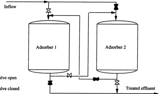
The treatment facility consists of two adsorber vessels in series filled with Granular Activated Carbon (Figure 4-1, Model 7.5 of Calgon Carbon Corporation). Each tank, 7.5

ft in diameter and 10 ft carbon depth, contains 10,000 lb of activated carbon. This system

of two downflow, fixed-bed adsorbers in series is the simplest and most widely utilized design for groundwater treatment applications (Stenzel et al., 1989). Two vessels in series assure that the carbon in the first vessel is completely exhausted before it is replaced, thus contributing to the overall carbon efficiency. The removed carbon is then transported off-site for reactivation.

The CS-4 plume water contains little suspended solids (E. C. Jordan, 1990). Therefore, filtration (e.g. sand filtration) of the plume water in order to prevent plugging of the subsequent treatment steps is not required. Although the suspended solid content in the influent is low, the carbon needs to be backwashed periodically. The installed backwash tank, 12 feet in diameter, contains 11,200 gallons of clean water. This allows backwash for 20 minutes with 560 gpm.

Inflow

Adsorber 1

77I1~~

Adsorber 2

D4 valve open

a

Figure 4-1: GAC configuration at CS-4.

Ir-

-I

---Metals such as iron or manganese are not present in high concentrations in the plume water (E. C. Jordan, 1990). Hence, a treatment step for metal precipitation is not necessary.

4.2 Theoretical Background

4.2.1 General Considerations

GAC is a technology based on adsorption. The soluble or gas phase contaminants

(sorbates, in our case the chlorinated organic solvents) are removed from the water- or gas phase by contact with an interface, e.g. the activated carbon surface. Examination of a microscopic cross-section of activated carbon reveals a porous structure with a large internal surface area, where the sorbates can attach. Activated carbon is available in both powdered and granular form, but the latter is most commonly used for the removal of a wide range of sorbates from water (Metcalf & Eddy, 1991; La Grega et al., 1994).

An important feature is that the treatment of the water with GAC does not destroy the contaminants. The process includes only a transfer of the contaminants from the water to the solid phase. For final destruction of the contaminants, the exhausted carbon (i.e. when the adsorbed contaminants are in equilibrium with the dissolved contaminants in the influent, and thus no more contaminants can be adsorbed with respect to the inflow concentration) needs to be burned, resulting in oxidation of the contaminants.

4.2.2 Preparation and Reactivation of the Carbon

Activated carbon is prepared by producing a char from materials such as almond, coconut, walnut hulls, woods, or coal. This is done by burning the material with insufficient supply of air so that the hydrocarbons are driven off. Then, by exposing the char particle to an oxidizing gas of steam, air and CO2 at a high temperature, the char

develops a porous structure and is now called activated. The porous structure results in a large internal surface area in a range of 650 up to 1800 m2_{/gram of carbon. The chosen}

carbon for the CS-4 treatment facility, Calgon F-300, has a internal surface area of approximately 1000 m2/g (EPA, 1971).

Once exhausted, carbon can be reactivated by dewatering it and then oxidizing the organic matter in a furnace at temperatures of about 870 -980 'C (1600 - 1800 'F). This results in removing the sorbed contaminants from the carbon surface. But through the reactivation process, about 5-15% of the carbon gets destroyed. Also, the adsorption capacity of reactivated carbon is slightly less than that of virgin carbon (Metcalf & Eddy, 1991). An alternative to thermal reactivation is solvent reactivation (e.g. with acetone, dimethylformamide).

4.2.3 Adsorption Capacity

Adsorption equilibrium is attained when the rate of adsorption onto the solid surface equals the rate of desorption from the solid surface back to the water phase (Neely and Isacoff, 1982). The quantity of adsorbate that can be taken up by an adsorbent (adsorption capacity) is a function of both the characteristics and concentrations of adsorbate as well as the temperature (Metcalf & Eddy, 1991). Thus, the adsorption capacity can be described as an equilibrium relationship between the moles of sorbate (i.e. contaminants) adsorbed per unit mass of sorbent (i.e. carbon) and the concentration of sorbate remaining in solution (Schroeder, 1977). Since these relationships are given for a constant temperature, they are called isotherms.

Equations that are commonly used to describe the experimental isotherm data were developed by Freundlich, by Langmuir and by Brunauer, Emmet and Teller (BET isotherm). While both Langmuir and BET isotherms are based on theoretical developments, the Freundlich isotherm model is an empirical relationship. The latter is used most commonly to frame the adsorption on activated carbon mathematically:

x = K

M

M (1)

X = mass of contaminant adsorbed (mg) M = mass of carbon (g)

K, n = empirical constants to fit curve to data (Freundlich constants, K in L/g)

Ci = concentration in solution after adsorption equilibrium is reached, which equals the influent concentration (mg/L)

where note that where Ce = V = (2) effluent concentration (mg/L) volume of solution (L)

Therefore, the required mass of carbon for each liter of treated with information on K and n.

water can be calculated

Compared to batch tests in the laboratory which are used to develop isotherms, full scale units normally don't reach equilibrium since the contact time of the water in the carbon vessel is too short (Metcalf & Eddy, 1991). Although reported isotherm data may also not reflect equilibria, the contact times there typically are longer. Also, isotherm lab tests are conducted with virgin carbon, under steady conditions (temperature, pH, etc.), and allowing no biological activity building up. These conditions are usually not met in operating units. Therefore, it is important to account for the reduction of the adsorption capacity for field scale units.

4.2.4 Multicomponent Solutions

In water treatment, the ideal case of one adsorbate being removed onto an adsorbent is seldom encountered. The objective of adsorption in most real systems is to remove several adsorbates at the same time. This complicates both the theoretical picture of

equilibrium among adsorbates and adsorbent and Ihe ability of the engineer to apply the theory in practice (Montgomery, 1985). Typically, there is a depression of the adsorptive capacity of any individual compound in a solution of many compounds (since the compounds are competing for sorption sites). However, if the concentrations of the solutes in the mixture are low, one may expect no significant decrease in the adsorption behavior of the organic molecules, since contaminant molecules are not likely to encounter competing molecules.

Several mathematical models have been developed to describe multicomponent adsorption behavior (e.g. Radke and Prausnik, 1972 (IAS model); Baldauf, 1978; Crittenden and Weber, 1978; DiGiano et al., 1978). The model of DiGiano and co-workers (1978) allows direct computation of the solute loading from known concentrations in the mixture:

n'-n

q=

_{ki Ci}

_{N(

_"

_kCini

₍₃₎

Where Ci = concentration of solute i in a mixture

ki, ni = Freundlich constants (Kf, n ), describing single solute adsorption k', n'= average ki and ni constants, respectively

N = number of solutes in mixture

Compared to actual measurements, this model provides a good prediction of the adsorption behavior of a multicomponent mixture especially if the contaminants are at low concentrations (DiGiano et al., 1978).

4.2.5 Kinetics of Adsorption

The rate of adsorption is another important issue to address in order to understand and effectively design carbon units. It may influence the required contact time and therefore the influent flowrate to give sufficient time to capture the solutes.

The adsorption of organic contaminants takes place in three steps: 1) macrotransport, 2) microtransport, and 3) adsorption. Macrotransport is referred to as the movement of the molecules through the water to the liquid-solid interface by advection and diffusion. Microtransport involves the diffusion of the molecules through the micropore system of the GAC granule to the adsorption sites. And the third step, adsorption, finally describes the attachment of the organic molecules to the carbon (Faust and Aly, 1987). The overall rate therefore will be controlled by the slowest step. Generally speaking, macrotransport seems to be the rate-limiting step in systems that have poor mixing, dilute concentrations of adsorbate, small particle sizes of adsorbent, and high affinity of adsorbate for adsorbent (Helfferich, 1962). In contrast, microtransport limits the overall transfer for those systems that have good mixing, large particle sizes of adsorbent, high concentration of adsorbate, and low affinity for adsorbent (Helfferich, 1962).

The required contact time of the contaminated water with the GAC (empty bed contact time, EBCT) is a function of these parameters. Generally, after an initial rapid decrease in carbon usage rate with increasing EBCT, the curve flattens and no significant reduction in usage rate is gained with increasing contact time (Faust and Aly, 1987). The shape of the curve depends on the particular carbon, the contaminant concentrations, and contaminant characteristics. Most EBCT studies are conducted with contact times up to 1 hour, since EBCTs over 1 hr are considered impractical for field units (Faust and Aly, 1987).

4.3 Adsorption Capacity of GAC at CS-4

Different researchers report different values for the Freundlich constants Kf and 1/n (Dobbs and Cohen, 1980; Weber, 1981; Benedict, 1982; Love and Eilers, 1982; Crittenden et al., 1985). A list of them can be found in Appendix B. Table 4-1 gives values for each of the contaminants of interest. These values (Dobbs and Cohen, 1980) are chosen as they are often cited in the literature and also represent the values with which the existing GAC was designed. For a given inflow concentration of the contaminant (for the calculations in Table 4-1 the maximum encountered values at CS-4 are chosen), the adsorption capacity at equilibrium can be estimated by using equation 1, chapter 4.2.3.

From isotherms for the F-300 carbon of the carbon supplier, Calgon Carbon Corporation (Appendix C), Kf and 1/n values were estimated and are also included in Table 4-1 in order to compare the literature values. The adsorption capacity at equilibrium with influent concentration is calculated using equation (1) and the influent concentration as shown in the following example (for PCE, literature values):

MX Kf Cil/n = 50.8-0.0620.56 = 10.7mg / g

Table 4-1: Freundlich constants from Dobbs and Cohen, (1980) and Calgon Carbon Corporation (1996). Capacities are calculated for maximum contaminant concentrations encountered at CS-4.

Literature Clgon Carbon'Corporation ontmitniaini t Ky /i Ads·ptionM Adsoirption K 1/n

concentration capiaciteat capacityat

ig/L) equilibriumtn ith equilibrium

inflient conc..: _ (L/g), - (mg/g). (•.g/g) ::.(Li.g) _ ' PCE (0.062) 50.8 0.56 10.7 44.1 134.0 0.40 TCE (0.032) 28 0.62 3.3 9.9 50.0 0.47 DCE (0.026) 3.1 0.51 0.5 1.9 13.0 0.52 TeCA (0.024) 10.6 0.37 2.7 1.2 11.2 0.60

4.3.2 Scenarios of Influent Concentration

The size of every GAC facility depends on two major parameters. The first one is the

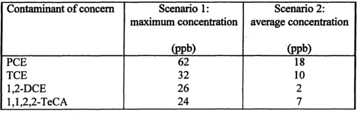
flowrate of water that has to be treated. As seen in Appendix F, the selected flowrate is 140 gpm. The second major parameter is the range of inflow concentrations of contaminants of concern. Since only about 20 samples determine the range of contaminant concentrations, this range is uncertain. To get a better feel about how the treatment system behaves with respect to different inflow concentrations, the following estimations of carbon usage are made for two different scenarios of plume concentrations: The two scenarios are defined as follows (Table 4-2):

* Scenario 1:

* Scenario 2:

Assuming the maximum concentrations (e.g. PCE @ 62 ppb) throughout the whole plume. This scenario represents the worst case.

Assuming average concentrations (e.g. PCE @ 18 ppb) throughout the whole plume.

The concentrations for scenarios 1 and 2 are the maximum and average values from the field observations, respectively, as presented in chapter 3.2.2.

Table 4-2: Two scenarios for influent concentrations.

While Table 4-2 represents the concentrations in the plumewater, the actual contamination of the extracted water which will flow into the treatment system, is

smaller. Through modeling of the behavior of the well fence, L6pez-Calva (1996) (Appendix F) determined that for the overall pumping rate of 140 gpm, only 43% of the extracted water is coming from the plume. The rest is clean water, coming from clean parts of the aquifer. Therefore, the inflow concentrations to the treatment facility are the concentrations of Table 4-2 multiplied by a factor of 0.43 (Table 4-3).

Table 4-3: Inflow concentrations to treatment facility, scenarios I and 2.

Contaminant of concern Scenario 1: Scenario 2: maximum concentration average concentration

(ppb) (ppb)

PCE

27

8

In order to determine the multicomponent loading rate (LR), i.e. the loading rate of the four contaminants together, and following the general consideration in chapter 4.2.4, the loading rate was calculated using different methods. The loading rate (lb carbon/1000 gal of water) is the amount of carbon which is used for the treatment of 1000 gallons of extracted water. Following equation 2, chapter 4.2.3, the theoretical loading rate with respect to influent concentrations of each contaminant was estimated. For that, adsorption capacities at equilibrium (mg/g, Table 4-1) are needed. As an example, the loading rate for PCE are calculated below, using literature Freundlich constants.

1. Calculation of adsorption capacity at equilibrium with influent concentrations (0.062

mg/L), using Freundlich values of 50.8 for Kf and 0.56 for 1/n: X = _{Kf Cil/n=50.8 -0.0620-}5 6

= 10.7mg / g M

2. To calculate the loading rate LR, an acceptable effluent concentration (at equilibrium)

needs to be assumed (e.g. 0.005 mg/L, MCL). In order to approximate field conditions

where effluent concentrations are zero at the beginning of the treatment process, but then

increase with time until the design effluent concentration is reached (assume linear

increase), equation (2) is modified to equation 2a.

X =Ci- V (2a)

The loading rate LR can thus be calculated as

1

C.

L

_.00221b

SLR = 0.062 005mg / L I 1000gal

X/M"( 2) =10.7mg / g -20.264gal g

LR = 0.0471b / 1000gal

Following the discussion in chapter 4.2.4, the loading rate of the multicomponent mixture of solutes must be estimated. What needs to be considered is the fact that the contaminants do not adsorb equally well. The least sorbable will break through first. A high loading rate for a contaminant (which corresponds to a low adsorption capacity at equilibrium with influent concentrations) indicates that the contaminant will break through early. The overall loading rate is thus determined by the contaminant with the highest loading rate. Since for given influent concentrations and effluent target levels the LR is a function of the adsorption capacity at equilibrium (X/M), this measure of how much of the contaminant can be adsorbed to the carbon needs to be calculated.

The estimation of the adsorption capacity at equilibrium (mg/g) of the contaminants in the mixture was approached by using four different methods and comparing them. The methods are:

1. Assuming that the contaminants are not influencing each other since their concentrations are low, the capacities are calculated using equation 1, chapter 4.3.2. Freundlich values from literature were used (Table 4-1).

2. The adsorption capacities of the contaminants are determined by using the competitive model as described in chapter 4.2.4 (equation 3). Freundlich values from literature are used.

3. Similar to method 1, but using Freudlich values calculated from the Calgon

isotherms (Table 4-1).

4. Similar to method 2, but using Freudlich values calculated from the Calgon isotherms.

The overall loading rate is determined by the contaminant which breaks through first. Table 4-4 shows the results of the calculations for the four methods with the inflow concentrations of scenario 1. In method 1, DCE is expected to break through first (lowest adsorption capacity at equilibrium), but this is not important because the influent concentration and therefore also the effluent concentration is below the MCL. Then, TeCA will break through at 2 ppb. While at the same time also TCE may break through (similar X/M as TeCA), PCE is probably still fully "captured" by the carbon (high X/M). The overall loading rate is thus determined by either TeCA or TCE, and was approximated to be approximately 0.05 lb/1000 gal (Table 4-4).

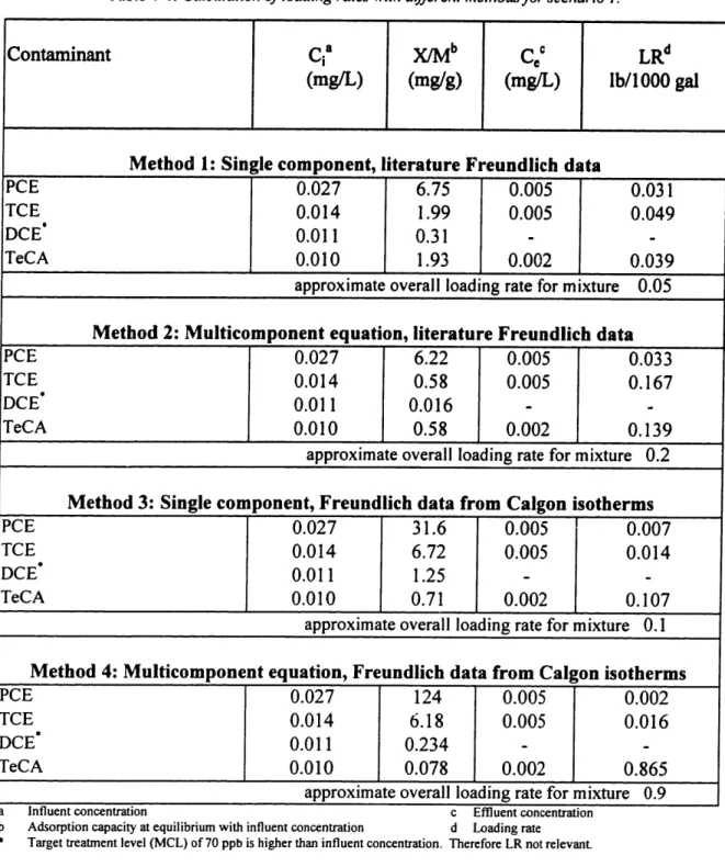
Table 4-4: Calculation of loading rates with different methods for scenario I.

Contaminant Ca X/Mb C c _LRd

(mg/L) (mg/g) (mg/L) lb/1000 gal

Method 1: Single component, literature Freundlich data

PCE 0.027 6.75 0.005 0.031

TCE 0.014 1.99 0.005 0.049

DCE* 0.011 0.31 -

-TeCA 0.010 1.93 0.002 0.039

approximate overall loading rate for mixture 0.05

Method 2: Multicomponent equation, literature Freundlich data

PCE 0.027 6.22 0.005 0.033

TCE 0.014 0.58 0.005 0.167

DCE" 0.011 0.016 -

-TeCA 0.010 0.58 0.002 0.139

approximate overall loading rate for mixture 0.2

Method 3: Single component, Freundlich data from Calgon isotherms

PCE 0.027 31.6 0.005 0.007

TCE 0.014 6.72 0.005 0.014

DCE 0.011 1.25 -

-TeCA 0.010 0.71 0.002 0.107

approximate overall loading rate for mixture 0.1

Method 4: Multicomponent equation, Freundlich data from Calgon isotherms

PCE 0.027 124 0.005 0.002

TCE 0.014 6.18 0.005 0.016

DCE* 0.011 0.234 -

-TeCA 0.010 0.078 0.002 0.865

approximate overall loading rate for mixture 0.9

Influent concentration c Effluent concentration

Adsorption capacity at equilibrium with influent concentration d Loading rate Target treatment level (MCL) of 70 ppb is higher than influent concentration. Therefore LR not relevant.

In method 2, DCE is also going to breakthrough first, but this is again not relevant. TeCA or TCE break through next (similar capacities), while according to the PCE adsorption capacity, PCE will still be adsorbed. The overall loading rate for the mixture is again determined by TeCA of TCE and was approximated to be 0.2 lb/1000 gal. In

method 3, TeCA had the lowest adsorption capacity and was expected to break through

first and thus determining the loading rate of about 0.1 lb/1000 gal. In method 4, the

adsorption capacities follows a similar trend to that observed in method 3. The overall LR

is thus about 0.9, which is much higher than the one for the other three methods.

All but the fourth method show similar overall loading rates between 0.05 and 0.2

lb/1000 gal. For the following calculations of the carbon usage rate of the GAC, it was

therefore assumed that the overall loading rate is approximated by 0.1 lb/1000 gal.

For scenario 2, analogous loading rate estimations were made. The values of the

calculations are shown in Appendix E. The overall loading rate is expected to be 0.05

lb/1000 gal.

4.3.4 Design Loading Rates

Considering the nonideal situation of a field scale carbon unit compared to a lab test as

described in chapter 4.2.3, the adsorption capacity of the full-scale column is some

percentage of the theoretical adsorption capacity found from the isotherms. The time

needed by the water to flow through one vessel was calculated to be 18 minutes (EBCT,

Calgon Carbon Corporation, Appendix D). Since this typical contact time gives only

limited time to the contaminants to adsorb, the effective capacity can be assumed to be

approximately 25 to 50 % of the theoretical one (Metcalf & Eddy, 1991). The design

loading rate was hence assumed to be the theoretical loading rate multiplied by the factor

2.5, which corresponds to 40% (Table 4-5).

Table 4-5: Calculation of design loading rates LRfor the two scenarios.

Scenario Theoretical LR Design LR (lb/1000 gal) (lb/1 000 gal)

1 0.1 0.25

4.3.5 Carbon Exchange Rate

The

_{carbon usage rate dictates how often one vessel containing the carbon has to be}

replaced. The vessel contains 10,000

lb

of activated carbon. The flowrate of extracted

water, which has to be treated, is 140 gpm. Table 4-6 summarizes the calculations. It can

be seen that in the case with the maximum inflow concentrations (scenario

1),

one carbon

vessel has to be exchanged approximately every two months. Therefore, 1.8 vessel

changes are required every year. For scenario 2, it was expected that only every 13

months a carbon vessel is exhausted. This results in 0.9 vessel changes per year.

Table 4-6: Carbon usage rate for two diferent scenarios of plume concentrations.

Scenario 1 Scenario 2

Design loading rate (lb/1000 gal) 0.25 0.13

Daily carbon use (lb/day) 50 25

Exchange of carbon after (month) 7 13

Number of vessel exchanges per year 1.8 0.9

4.4 Cost Estimation

This chapter encompasses an estimation of carbon exchange cost if the GAC will be operated until the CS-4 area is completely remediated, which, according to the results of the team-project, is in approximately 90 years.

Due to the carbon exchange/reactivation cost, operation and maintenance (O&M) costs of

GAC systems are generally relative high. Typically, O&M cost of $0.48 - $2.52 per

1,000 gallons of treated water must be expected and depend mainly on the influent

concentrations and characteristics of the contaminants. Reducing influent concentrations is thus a most efficient way to reduce O&M costs.

In order to transform long-term carbon exchange cost to today's values, the net present worth was calculated, using equation (4):

PW=- A l01,+) n 1(4)

where n = Number of years

i = Interest rate (assumed to be 5%) PW = Present worth

A = Annual cost

For the assumed pumping duration of 90 years, the factor to calculate the present worth (parenthesis in equation 4) equals 19.8. The costs for 90 years (PW) are thus calculated

by multiplying the annual cost (A) by 19.8.

The total carbon exchange/reactivation costs involve the exchange of the carbon, transport off site, reactivation and transport back to the treatment facility. The following rates were assumed (Calgon Carbon Corporation, 1996):

* Reactivation/Replacement: $ 1.13 per lb of carbon (10,000 lb to be exchanged each time).

* Transport to regeneration plant: $ 2.48 per mile round-trip. The nearest regeneration facility to Cape Cod/CS-4 is located about 700 miles away in Pittsburgh or New Jersey. This results in about $ 2,000 each round-trip.

With these assumptions, the carbon exchange cost for the required pumping years are presented in Table 4-7. It should be emphasized at this point that these values do not represent the total operation and maintenance costs. For that, additional cost would have to be added for monitoring, backwash, and energy requirements.

Table 4- 7: Total estimated carbon exchange cost (net present value) over expected duration ofpumping.

Scenario 1 Scenario 2 Changes of vessel per year 1.8 0.9

Carbon exchange cost per year ($) 25,000 12,000

Required pumping years 90 90

Present worth factor 19.8 19.8

Total carbon exchange cost ($) 484,000 242,000

The difference in total carbon exchange cost between scenario 1 (maximum inflow concentrations) and scenario 2 (average inflow concentrations) is about $ 250,000 or a factor of 2. These results show the importance of a good knowledge of the average contaminant concentrations in the plume in order to predict the long-term carbon exchange cost and also the operation and maintenance cost in general.

5. Technology Review

Considering the cost estimates for carbon exchange as shown in chapter 4, the question of alternatives to the existing technology or its economical optimization and enhancement was addressed. The first section (chapter 5.1) summarizes how the GAC was selected as an interim remedial technology, while in the second section (chapter 5.2), different types of technology which might be suitable alternatives for the CS-4 clean-up are briefly presented.

5.1 GAC Evaluation

5.1.1 Evaluation Criteria for GAC Selection

At this point, it is important to be aware of the nine evaluation criteria, which were used to select the CS-4 interim GAC technology (E. C. Jordan Co., 1990; ABB ES, 1992a):

(1) Overall protection of human health and the environment

(2) Compliance with ARARs (Applicable or Relevant and Appropriate Requirement) (3) Long-term effectiveness and permanence

(4) Reduction of mobility, toxicity or volume through treatment (5) Short-term effectiveness

(6) Implementability

(7) Cost

(8) State acceptance

(9) Community acceptance

5.1.2 Other Technologies Considered

The other technologies considered for the interim remedial technology are briefly reviewed. Of the 13 remedial technologies screened in the Feasibility Study (E. C. Jordan, 1990), five were selected and retained for detailed analysis. For further evaluation, they were compared against the above nine criteria.

1) Air stripping followed by activated carbon

By bubbling air through the contaminated water, the VOCs partition into the air, causing

in contaminant transfer from the water to the gaseous phase. The gas is then treated by vapor-phase carbon adsorption to meet with the regulatory limits. The advantage of this concept is that carbon adsorption is sometimes more efficient in treating gases than liquids, depending on inflow characteristics (O'Brien and Stenzel, 1984; McKinnon and Dyksen, 1984).

2) UV Oxidation

An oxidant (e.g. peroxide, ozone) is added to the water which thus oxidizes the contaminants, yielding less harmful chemicals. The reaction rate of this process is enhanced by exposing the water to ultraviolet (UV) light.

3) Spray aeration

Spray aerators sprinkle the extracted water through the air, forming tiny droplets. Thus by extending the air-water contact area, the contaminants can evaporate into the air at a faster rate. As a result, the VOCs don't get actually destroyed but only vaporized and dissipated into the atmosphere.

4) Otis Wastewater Treatment Plant

The contaminated groundwater is treated at the Otis Wastewater Treatment Plant (WWTP), where it is subject to the same biological treatment as municipal sewage water. Although the WWTP was not designed to treat VOC-contaminated groundwater, existing processes may be able to remove the VOCs (Smith et al., 1993). Volatilization in the

various process steps would be the predominant removal mechanism to air.

These alternatives were not only compared against the above nine criteria, but also against the "no action" alternative. The contaminant plume would not be removed from the aquifer and only a monitoring program implemented (E. C. Jordan Co., 1990; ABB