HAL Id: hal-02910108
https://hal.archives-ouvertes.fr/hal-02910108
Submitted on 31 Jul 2020
HAL is a multi-disciplinary open access
archive for the deposit and dissemination of
sci-entific research documents, whether they are
pub-lished or not. The documents may come from
teaching and research institutions in France or
abroad, or from public or private research centers.
L’archive ouverte pluridisciplinaire HAL, est
destinée au dépôt et à la diffusion de documents
scientifiques de niveau recherche, publiés ou non,
émanant des établissements d’enseignement et de
recherche français ou étrangers, des laboratoires
publics ou privés.
A general analytical method for interface normal
determination in TEM A general analytical method for
interface normal determination in TEM
Rui-Xun Xie, Melvyn Larranaga, Frédéric Mompiou, Nicolas Combe,
Wen-Zheng Zhang
To cite this version:
Rui-Xun Xie, Melvyn Larranaga, Frédéric Mompiou, Nicolas Combe, Wen-Zheng Zhang. A
gen-eral analytical method for interface normal determination in TEM A gengen-eral analytical method
for interface normal determination in TEM. Ultramicroscopy, Elsevier, 2020, 215, pp.113009.
�10.1016/j.ultramic.2020.113009�. �hal-02910108�
Highlights
A general analytical method for interface normal determination in TEM
XIE Rui-Xun,LARRANAGA Melvyn,MOMPIOU Frédéric,COMBE Nicolas,ZHANG Wen-Zheng • We present a general method to determine the interface normal from arbitrary orientations. • We developed a general model of interface projection, including existing methods as special cases. • The method is proved to be robust, efficient, and scalable in different situations.
A general analytical method for interface normal determination in
TEM
XIE
Rui-Xun
a,
LARRANAGA
Melvyn
b,
MOMPIOU
Frédéric
b,
COMBE
Nicolas
band
ZHANG
Wen-Zheng
aaKey Laboratory of Advanced Materials (MOE), School of Materials Science and Engineering, Tsinghua University, Beijing 100084, PR China bCEMES-CNRS, Université de Toulouse, 29 rue J. Marvig, 31055 Toulouse, France
A R T I C L E I N F O
Keywords:
Transmission Electron Microscopy (TEM) Trace analysis
Interface Crystallography
A B S T R A C T
This paper presents a new analytical method to determine interface normals from a series of bright/dark field images taken from arbitrary orientations. This approach, based on a general geometrical model of interface projection, provides a generalized formulation of existing meth-ods. It can treat an excessive number of inputs, i.e. orientation conditions. Given 6 or more sets of inputs, even with considerable experimental errors, we prove that this method is still very likely to yield results with satisfactory trueness. The robustness of the method can thus allow its implementation in problems dealing with a large amount of data. We show that this method can also be applied to determine 1D features or to check the planarity of microstructural features.
1. Introduction
Transmission electron microscopy (TEM) is a powerful tool to examine a variety of defects in materials, including point defects (zero dimension, 0D), dislocation lines (1D), interfaces (2D) and inclusions (3D). Since TEM images are 2D projections of the 3D space, the geometrical features of non-0D defects, e.g., their shapes, must be reconstructed from their projections on the observation plane. The identification of 3D inclusions, curved lines or curved planes is a cumbersome work [1][2]. However, many 1D or 2D defects, e.g., interfacial dislocations or faceted interfaces, often have preferred orientations. They can be considered as straight lines or flat planes. Accurately determining their crystallographic orientations is fundamental to unravel the mechanism of associated microstructure evolution [3]. In this context, the problem is restricted to the line direction or the interface plane normal determination, using a technique called trace analysis [4][9].
The concept and methods of trace analysis using TEM were clearly introduced in the well-known book by Hirsch et al. [4]. A line feature is always on the plane defined by its projection and the electron beam direction. Therefore it can be determined if observed from two directions. However, the projection of a planar feature usually contains the projection of two traces, the intersections of the interface with two foil surfaces, separated by a certain width. An interface can be directly determined at its edge-on condition, where the projection width is zero and the interface
normal lies in the viewing screen [4]. Since an edge-on condition often carries non-negligible uncertainty, several modifications were later proposed to improve the accuracy, such as the single edge-on method [9][5], the double edge-on method [10][11], and the trace & edge-on method [12]. Despite their good accuracy, these methods are not easy to use, as finding an exact edge-on condition is usually time consuming or even impossible if it is out of the tilting range of the sample holder.
An edge-on condition is not always necessary, if the interface contains an additional sharp line feature, such as a straight dislocation line [5][6][7] or an intersection with another plane [8], using the so-called double-trace method. The orientations of both trace and line feature in the plane can be measured by the trace analysis method of 1D features. Then one can obtain the interface normal by making a cross product of the line and the trace direction. However, additional line features are not always present, which limits the application of this method.
When the condition for the double-trace method is not satisfied, the projection width can be used to calculate interface normals at arbitrary orientations. In this approach, the trace direction is assumed to lie on the screen plane at zero tilt. The interface normal can be determined, once the inclination angle between the foil surface and the interface is determined. Traditionally, this was done by measuring the foil thickness and the projection width of the interface at an orientation near to zero tilt [9]. Since this method contains considerable uncertainty, Zhang and Kelly [13] made an improvement by tilting the sample along the trace direction. But it is usually difficult to ensure the tilting axis exactly parallel with the trace direction. Qiu an Zhang [14] solved this problem on a single tilt holder by taking the angle between the trace and the tilting axis into consideration. In order to avoid ambiguous solutions, this approach still needs to track the trend of the projection width change during sample tilting. All these methods are based on the assumption that the upper and lower foil surfaces are both perpendicular to the electron beam direction at zero tilt. This may introduce systematic error when the foil has thickness variation or not flat.
Above methods are highly sensitive to experimental errors, since they rely on limited information — usually one or two sets of inputs (beam and projected trace directions, projection width). Particularly, the error could be greatly amplified by the cross product operation in double trace and double edge-on methods [12]. To improve the reliability, one may use excessive experimental data to calculate several solutions of the interface normal. The scattering of results can be plotted in a pole figure [12][14], but the selection of the final result and the estimation of its uncertainty are largely based on the operator’s experience.
In order to improve the accuracy of interface normal determination and simplify the TEM operation, we present here a close-form algorithm to optimize the result with multiple sets of inputs from arbitrary orientations. In this method, there is no specific requirements on the beam direction, nor conditions on the interface and the foil.
In Section 2, we will describe the methodology used to compute the interface normal. Section 3 will present experimental details, followed by Section 4 illustrating the applications of the present method. The results and method will finally be discussed in Section 5. The accuracy of the results will be adressed by an error analysis, and the method will be compared with other methods proposed in the literature. A generalization of our approach will be proposedat the end.
2. Geometrical model of interface projection
The approach presented below is a purely geometrical analysis of the orthogonal projection of planar features on the observation screen, without any requirement on the beam direction (projection direction) or the foil surface. It is based on the measurement of the interface width and apparent trace direction for different beam direction. The symbols used in the derivation and their meaning are listed inTable1.
Table 1
Definition of symbols1
Symbol Definition
𝒃e Reversed electron beam direction, unit vector
𝒏 Interface normal, unit vector
𝒓 Arbitrary vector in the screen plane, unit vector, 𝒃e⋅ 𝒓 = 0
𝒔 Foil surface normal, unit vector
𝒕 Trace direction, i.e., direction of the intersection between the interface and the
foil surface, unit vector 𝒕 = 𝒏 × 𝒔∕‖𝒏 × 𝒔‖
𝒕p Projected direction of 𝒕
ℎ Foil thickness
𝜂 Azimuth angle from 𝒙 axis of the screen to 𝒕p
𝑑 Real interface width, i.e., real distance between traces
𝑤 Projected interface width, i.e., distance between projected traces
𝑖 Input number, index, 1 ≤ 𝑖 ≤ 𝑚 𝑚 Total number of inputs
Rx(𝜃), Ry(𝜃), Rz(𝜃) Right-handed rotation matrix with rotation angle 𝜃 about 𝑥, 𝑦, 𝑧 axis respectively sgn(𝑖) A function that gives a value of ±1 respect to the sign of 𝒏 ⋅ 𝒃ei
A flat interface has two traces, the intersections with upper and lower foil surfaces. Firstly, let us assume the two foil surfaces to be parallel planes, resulting in two parallel traces separated by a certain width 𝑑. This case is
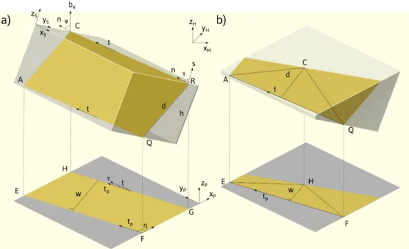
Figure 1: Geometrical description of interface projection. (a) Parallel traces case: The interface 𝐴𝑄𝑅𝐶 is projected on the viewing screen, giving the projection 𝐸𝐹 𝐺𝐻. The inset is the cross section view along the trace direction. (b) Non-parallel traces case: A traceable point 𝐶 on the interface and a trace 𝐴𝑄 are projected to the viewing screen, giving the projection
𝐸𝐹 𝐻.
shown inFigure1a, where the interface is enclosed by the red parallelogram 𝐴𝑄𝑅𝐶. Line 𝐶𝑅 and 𝐴𝑄 are upper and lower traces of the interface, intersections between the foil surfaces (orange planes) and the interface. The blue parallelogram 𝐸𝐹 𝐺𝐻 is the projected interface on the screen. Areas of these parallelograms, 𝑆𝐴𝑄𝑅𝐶 = 𝑑|𝐴𝑄| and
𝑆𝐸𝐹 𝐺𝐻 = 𝑤|𝐸𝐹 |, are related by 𝑆𝐸𝐹 𝐺𝐻 = 𝑆𝐴𝑄𝑅𝐶cos 𝜓, where 𝜓 is the angle between reversed electron beam direction 𝒃e and interface normal 𝒏. Since |𝐸𝐹 | is the projection of |𝐴𝑄|, they are related by |𝐸𝐹 | = |𝐴𝑄| cos 𝜏,
where 𝜏 is the angle between trace 𝒕 and its projection 𝒕p.
When the foil is bent or has a wedge shape, the assumption of parallel foil surfaces is no longer valid. Because of this, trace 𝐴𝑄 and trace 𝐶𝑅 are not parallel, 𝐴𝑄𝑅𝐶 in Figure1is no longer a parallelogram (Figure1b). However, if a point on the interface can be tracked, it is still possible to resolve the relationship between 𝑑 and 𝑤. As shown in
Figure1b, by tracking point 𝐶 on the interface 𝐴𝑄𝐶, one can redefine 𝑑 as the distance between 𝐶 and the trace 𝐴𝑄, intersection with one foil surface (orange plane), while the distance between the projected point 𝐻 and projected trace
𝐸𝐹 is measured as 𝑤. In this case, it is crucial to measure 𝑤 at the same position each time. The area of interface
The relationship of |𝐸𝐹 | = |𝐴𝑄| cos 𝜏 remains valid.
Therefore, no matter two foil surfaces are parallel or not, the interface projection width 𝑤 is always given by
𝑤= 𝑑cos 𝜓
cos 𝜏 (1)
Or alternatively using dot product:
𝑤= √|𝑑𝒏 ⋅ 𝒃e| 1 −(𝒃e⋅ 𝒕)2
(2) InEq. (2), 𝑤 and 𝒃ecan be measured, while 𝑑𝒏 and 𝒕 are unknown.
Vector 𝒕 can be determined from its measured projections 𝒕p’s at different 𝒃e’s, using:
[
𝒃e1× 𝒕p1 𝒃e2× 𝒕p2 ... 𝒃em× 𝒕p𝑚
]T
𝒕= 𝟎 (3)
When 𝑚 = 2,Eq. (3)is solved by using the cross product 𝒕 = (𝒃𝑒1× 𝒕𝑝1) × (𝒃𝑒2× 𝒕𝑝2). When the number of input
sets 𝑚 ≥ 3, it is an overdetermined homogeneous linear equation, and can to be solved by the least square method (LSM, see Appendix A).
The determination of 𝒕 allows to compute the non-linear part√1 −(𝒃e⋅ 𝒕)2inEq. (2), turning Eq. (2)into a linear problem. However, the width of interface projection, 𝑤𝑖, is always positive, while 𝒏⋅𝒃eicould be negative. Thus
sgn(𝑖), the sign of 𝒏 ⋅ 𝒃ei, is needed to remove the absolute sign inEq. (2). Using the fact that 𝑑𝒏 ⋅ 𝒕 = 0, a synthetic
formula incorporating the input measurements (𝑤𝑖,𝒃ei)can be derived:
⎡ ⎢ ⎢ ⎢ ⎢ ⎢ ⎢ ⎢ ⎢ ⎢ ⎢ ⎢ ⎢ ⎢ ⎣ 𝒃Te1 𝒃Te2 ... 𝒃Ten 𝒕T ⎤ ⎥ ⎥ ⎥ ⎥ ⎥ ⎥ ⎥ ⎥ ⎥ ⎥ ⎥ ⎥ ⎥ ⎦ (𝑑𝒏) = ⎡ ⎢ ⎢ ⎢ ⎢ ⎢ ⎢ ⎢ ⎢ ⎢ ⎢ ⎢ ⎢ ⎣ sgn(1)𝑤1 √ 1 −(𝒃e1⋅ 𝒕)2 sgn(2)𝑤2 √ 1 −(𝒃e2⋅ 𝒕)2 ... sgn(𝑚)𝑤𝑚 √ 1 −(𝒃em⋅ 𝒕)2 0 ⎤ ⎥ ⎥ ⎥ ⎥ ⎥ ⎥ ⎥ ⎥ ⎥ ⎥ ⎥ ⎥ ⎦ (4)
𝑚= 2,Eq. (4)is determined and two different solutions are expected. It is impossible to assess the actual one without additional information. When 𝑚 ≥ 3,Eq. (4)is overdetermined, and its residual error can be computed (see Appendix A). The uncertainty of sgn(𝑖) will give 2𝑚−1 solutions of 𝒏. The one with the minimum residual error is the best
solution, because an improper sgn(𝑖) would result in significantly large residual error. The contribution to the residual error from each set of input (𝑤𝑖,𝒃ei,𝒕p𝑖)can be quantified by the respective element in the residual vector ofEq. (4)
(see Appendix A). The element with the maximum absolute value and different sign from the others may indicate an abnormal input with significantly large deviation. One may drop this input and recalculate the result, which can reduce the residual error and improve the input consistency. Thus, with at least 3 different sets of experimental data (𝑤𝑖,𝒃ei,𝒕p𝑖), LSM will give the optimized solutions of 𝒕, 𝑑 and 𝒏.
The accuracy of the interface normal, which is the deviation between the determined value and the true value is an important concern. Unfortunately, the true value of 𝑑𝒏 is usually unknown, and needs to be estimated. The estimation of the true value is a range with a certain confidence, i.e., a confidence interval, which can represent the accuracy of the result, based on the internal consistency of inputs. In the present work, the 95% confidence interval of 𝑑 and that of 𝒏 can be calculated by the bootstrap method (see Appendix B) withEq. (4).
A C++ implementation of the present algorithm can be found in Supplementary Materials.
3. Experimental details
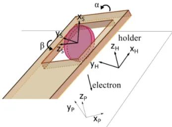
The present method was tested in two cases. In both cases, bright field images were recorded at different orientation conditions in an FEI Tecnai G2 20 TEM operated at 200 kV. Observations were performed using a double tilt sample holder with the coordinate conventions as shown inFigure2: the x-axis is parallel to the holder axis, and the y-axis is perpendicular to the x-axis and the beam direction. In the following, the subscriptsH,PandSdenote the indices in
holder, projection screen, and sample coordinate system, respectively . In the holder coordinate system, the sample is firstly tilted about the −𝒚 axis by angle 𝛽, and then tilted about the −𝒙 axis by angle 𝛼.
The rotation angle from holder 𝒙𝐻axis to the projection screen 𝒙𝑃axis is 𝜙 about 𝒛𝐻= 𝒛𝑃axis. This accounts for
the rotation of the image in the microscope column. Hence, the beam direction 𝒃eperpendicular to the screen and the
direction 𝒕pin the observation plane can be calculated using right-handed rotation matrices Rx(𝜃), Ry(𝜃), and Rz(𝜃),
Figure 2: Illustration of the holder coordinate system when the sample is mounted in a double-tilt holder.
𝒃e= Ry(𝛽)Rx(𝛼)[0, 0, 1]TH
= [sin 𝛽 cos 𝛼, − sin 𝛼, cos 𝛽 cos 𝛼]TS
(5)
𝒕p= Ry(𝛽)Rx(𝛼)Rz(𝜙)[cos 𝜂, sin 𝜂, 0]TP (6)
where 𝜂 is the azimuth angle between the projected trace and the 𝑥𝑃-axis on the viewing screen.
In the first experiment, a grain with two interfaces was investigated in a duplex stainless steel Fe-24.9Cr-7.0Ni-3.1Mo (wt%) sample prepared by the same procedure as reported in [15]. The images were taken in conditions where
𝜙= 90◦.
In the second case, a grain boundary with non-parallel traces was observed in an aluminum bicrystal with a mis-orientation close to a coincident Σ41 12.68◦< 0 0 1 > {5 4 0}. The sample was first ground to 50 microns using
SiC grain disks and then electro-polished to obtain electron transparency. The TEM foil was strained in-situ at c.a. 400◦C, as reported earlier in [? ] (ref missing). Plastic deformation leads to a complex microstructure of dislocations,
resulting in significant bending of the wedge foil and possible deviation from the original orientation.Eq. (5)andEq. (6)are still valid in this case, using here 𝜙 = 157◦forEq. (6).
4. Application examples
4.1. Measuring two interfaces with a double-tilt holder
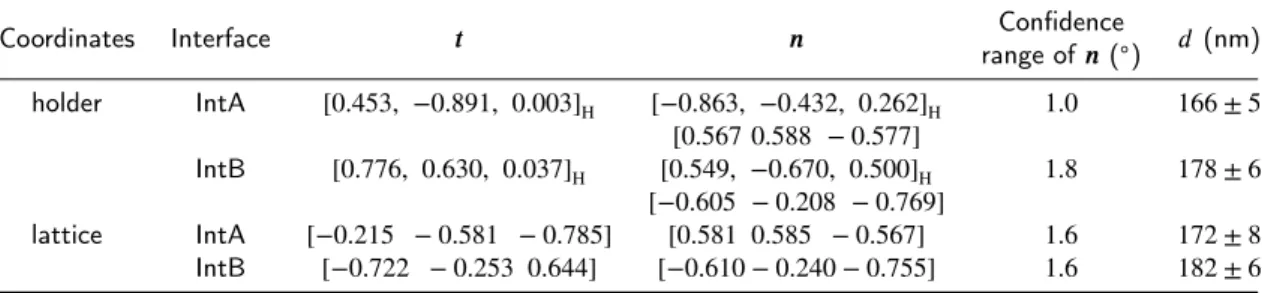
Figure3shows a series of bright field (BF) images of a faceted austenite grain (A) in a ferrite matrix (F) taken at different orientations. Two FCC/BCC facets, IntA and IntB, intersect and form a well defined corner. In order to show the ability to determine multiple interfaces, normals of these two facets are determined simultaneously, using 6 sets of inputs among 8 different imaging conditions. The determination was performed both in the holder coordinate system and in the lattice coordinate system. The former is more convenient to use, as it only needs tilt angles of the sample holder, while the latter, which requires the analysis of Kikuchi patterns, usually has better accuracy. The normal of IntA is determined byFigures3a∼f, and that of IntB byFigures3a ∼ e and3g.Figure3h, a near edge-on condition of both IntA and IntB, was only used to check the results.
The first step of the method is to determine 𝒕. The 𝒃e’s in holder coordinates were calculated with data inTable2
andFigure3, usingEq. (5)andEq. (6), while the 𝒕p’s of IntA and IntB are given by their azimuth angle with respect to
the 𝒙 axis ofFigures3a∼g. The lattice coordinates of 𝒃e’s and 𝒕p’s were defined in austenite using the Kikuchi patterns
shown inFigure3, as listed inTable2. Hence 𝒕 was determined by solvingEq.3in either coordinate system. The second step is to substitute 𝒃e’s, 𝒕, and 𝑤𝑖’s, intoEq. 4to solve 𝑑𝒏. By enumerating all the possibilities of
sgnA(𝑖), and sgnB(𝑖), 𝑑𝒏 and its residual error in both conventions are solved by LSM. Among them, the one with the
minimum residual error was chosen as the final result, whose sgn(𝑖) is shown inTable2. Then, the optimized results were calculated, as shown byTable3. The 𝒏’s in holder coordinates were transformed to lattice coordinates using the transformation matrix determined fromFigure3e2(see Supplementary materials).
The 𝒕’s of IntA and IntB in holder coordinates are almost in the 𝑥𝑂𝑦 plane, indicating that the foil was almost perpendicular to the beam direction at zero tilt. For each interface, the real width (𝑑) and the normal (𝒏) calculated from different coordinate systems show a good consistency. This means the holder coordinate system can be used instead of the lattice coordinate system to simplify the process while reserving the accuracy. The correctness of 𝒏 is verified by tilting both interfaces to a near edge-on condition (Figure3h), where the interface normal 𝒏 can be determined by 𝒃e× 𝒕p. Using the data ofFigure3hinTable2, the normal of IntA is [0.562 0.592 − 0.579], and that
Figure 3: BF images of the interfaces and the corresponding Kikuchi patterns taken in austenite at different tilt angles. The 𝛼 and 𝛽 tilt angles are reported in the bottom right. The projection widths and the azimuthal angle of both IntA and IntB interfaces are also indicated. Arrows in the Kikuchi patterns indicate the 𝒃e× 𝒕p directions of IntA and IntB.
Hence, the present method is able to accurately determine multiple interfaces simultaneously, either in the holder or lattice coordinate system.
4.2. Measuring a grain boundary with non-parallel traces
Figure4shows a series of BF images of an interface with non-parallel traces in an Al bicrystal sample taken at different tilt angles. The tracked point (pointed out by arrows) is defined by the position where the lower trace (dotted line) starts to deviate.Figures4a∼eare used to solve the interface normal, whileFigure4fis a near edge-on condition
Table 2
Directions in lattice coordinates from the Kikuchi patterns inFigure3and sgn(𝑖) for solvingEq. (4)
Figure 𝒃e IntA 𝒕p IntB 𝒕p sgnA(𝑖) sgnB(𝑖) 𝑤A𝑖 𝑤B𝑖 𝛼( ◦) 𝛽(◦) 3a [-0.811 0.485 0.327] [0.546 0.427 0.721] [0.249 0.792 -0.558] -1 +1 72 38 -37.86 27.22 3b [-0.629 0.147 -0.763] [-0.250 0.891 0.378] [0.772 0.239 -0.590] +1 +1 33 175 35.23 25.19 3c [-0.107 0.628 -0.771] [0.186 0.774 0.605] [0.963 -0.128 -0.238] +1 +1 130 108 30.53 -27.39 3d [-0.281 0.951 0.130] [0.485 0.023 0.874] [0.691 0.295 -0.660] +1 -1 73 27 -29.90 -27.28 3e [-0.465 0.341 -0.817] [-0.048 0.912 0.408] [0.885 0.157 -0.438] +1 +1 81 149 35.48 4.56 3f [-0.677 0.684 0.272] [0.597 0.295 0.746] [0.457 0.680 -0.574] -1 not used 26 - -37.32 6.65 3g [-0.654 0.704 0.277] [0.612 0.277 0.741] [0.469 0.665 -0.582] not used +1 -0 -38.01 4.51 3h [-0.592 0.776 0.219] [0.578 0.220 0.786] [0.541 0.584 -0.601] not used not used -- -34.12 -0.66 Table 3
Results of trace directions and interface normals
Coordinates Interface 𝒕 𝒏 Confidence
range of 𝒏 (◦) 𝑑 (nm) holder IntA [0.453, −0.891, 0.003]H [−0.863, −0.432, 0.262]H 1.0 166 ± 5 [0.567 0.588 − 0.577] IntB [0.776, 0.630, 0.037]H [0.549, −0.670, 0.500]H 1.8 178 ± 6 [−0.605 − 0.208 − 0.769] lattice IntA [−0.215 − 0.581 − 0.785] [0.581 0.585 − 0.567] 1.6 172 ± 8 IntB [−0.722 − 0.253 0.644] [−0.610 − 0.240 − 0.755] 1.6 182 ± 6
for verification. The trace 𝒕 of the interface in holder coordinates deviates from the 𝑥𝑂𝑦 plane, confirming that the foil is bent. Through a similar process as the previous example, the optimized result in holder coordinates is calculated as following: 𝒕 = [0.883, −0.348, 0.315]H, 𝒏 = [−0.473, −0.646, 0.600]H ∼ 2.4◦, and 𝑑 = 224 ± 12 nm. (what is
2.4◦?) Using the transformation matrix determined from a Kikuchi pattern (Figure S1), the lattice coordinates of the
interface normal is 𝒏 = [4.000 − 4.176 0.144] with 5.3◦deviation from [4 − 5 0]. Noting that the 95% confidence
range is 2.4◦, this deviation is considered to be the result of plastic deformation, rather than experimental errors. Using
Eq.5, the 𝒃eat the near edge-on condition inFigure4fis [0.278, 0.536, 0.797]H, which is almost perpendicular to the
interface normal with 0.1◦deviation. This edge-on condition confirms the result of 𝒏. Therefore, the present method
Figure 4: BF images of the interface with non-parallel traces at different tilt angles. The 𝛼 and 𝛽 tilt angles are reported in the top left. The widths between the tracked point (indicated by arrows) and the trace (dash line), and the azimuth angles of the trace (dash line) are also indicated.
5. Discussion
5.1. Accuracy of 𝒏
The use of the method presented here raises three questions concerning the accuracy of 𝒏: (i) is the true value of the interface normal inside the bootstrap confidence interval; (ii) what is the main error source on interface normal determination; (iii) what is the optimal number of input datasets for an acceptable accuracy. To answer these questions, statistical analysis was performed using simulated erroneous data.
The simulated datasets were generated in holder coordinates, using a 100-nm-thick virtual sample with two parallel surfaces normal to 𝒛. As the prerequisite, the true value of the interface normal 𝒏 must be known. Then, the 𝛼 and 𝛽 angles were randomly chosen in ±40◦range, and the true values of 𝑤 and 𝜂 were calculated. The dataset (𝛼, 𝛽, 𝜂, 𝑤)
was randomly varied to simulated the experimental error. The 𝛼, 𝛽 and 𝜂 angles were randomly varied in ±1◦range,
while the projection widths in ±5 nm range. With several erroneous datasets, the interface normal was determined, and the deviation from the true value, which is called trueness for clarity, was calculated.
In the first analysis, the interface normal was randomly chosen and determined with 6 sets of simulated data. This process was repeated 10000 times, and the true value was inside the bootstrap confidence interval for 9369 times. This agrees to the confidence level (95%) of the interval. The true value could be outside the confidence interval when the datasets (𝛼, 𝛽, 𝜂, 𝑤) have relatively large systematic error, as this problem cannot be figured out from the consistency
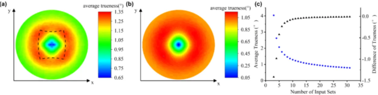
Figure 5: Statistical analysis of the trueness of the results.
(a) Distribution of the average trueness for interface normals chosen within the pole figure viewed from 𝒛 axis. 𝛼, 𝛽, 𝜂 and
𝑤have random errors. The beam directions reached by sample tilting are limited by dashed lines. (b) Same as (a) when the error is restricted to 𝑤. (c) The change of trueness with respect to the number of inputs for a fixed interface normal.
of the datasets.
In the second analysis, 4949 unit vectors evenly distributed on a hemisphere were used as known interface normals. For each normal, 6 arbitrary conditions (𝛼, 𝛽, 𝜂, 𝑤) were used to compute back an erroneous normal, and its trueness. Because the trueness is dependent on the orientation conditions, it was averaged over 10000 arbitrary condition sets for each known normal.
The results are plotted in a pole figure inFigure5a. It shows an 𝑚𝑚 symmetry due to the angular area covered by the sample tilt, limited by the dashed lines inFigure5a. The average trueness of interface normals ranges between 0.65◦and 1.35◦, but most of the value is due to the error on 𝑤 as shown inFigure5b, where the average trueness is
computed when varying only 𝑤. The ring-like shape of trueness inFigure5acan be understood by inspecting how errors affect the value of cos 𝜓 inEq. 4. Using ℎ = 𝑑 sin 𝛾 = 𝑑√1 − (𝒏 ⋅ 𝒔)2(Figure1ainset) andEq. 2, we can derive
cos 𝜓 = 𝒏⋅ 𝒃e= 𝑤
ℎ
√
1 −(𝒃e⋅ 𝒕)2sin 𝛾 (7)
When the interface normal 𝒏 moves from the center to the edge in the pole figure, statistically, sin 𝛾 =√1 − (𝒏 ⋅ 𝒔)2 will increase, making the value of cos 𝜓 more sensitive to the error of 𝑤. In other words, largely inclined planes in the foil are less precisely determined, because they statistically present orientation conditions where the projection width is small. Meanwhile, the increase in 𝜓 makes the direction of 𝒏 less sensitive to the error of cos 𝜓, as d𝜓 = −d(cos 𝜓)∕ sin 𝜓. The two effects having opposite variations, this leads to a trueness distribution with a maximum value in a ring area inclined about 54◦ with the foil normal (Figure5b). In common cases, the projection of the
the error of 𝒏 mainly comes from the error of 𝑤.
In the third analysis, the interface normal was fixed to [−0.547, 0.514, 0.661]H, an orientation with the worst
trueness inFigure5a, while the number of input datasets varied from from 3 to 15. The average of trueness were computed, again by randomly varying the condition sets over 10000 configurations. As shown inFigure5c, the trueness of 𝒏 would reach 1.7◦with 6 sets of inputs. It would reach 1.5◦with 8 sets of inputs, but barely improves afterwards.
Based on the above analysis, 6 to 8 sets of inputs would be the optimal choice.
In practice, it is trivial to reach the data quality (±1◦, ±5nm) in this analysis, and hence to get the results with the
corresponding accuracy. Moreover, data quality can even be improved by image measurements at higher magnification, and by using Kikuchi patterns.
5.2. Comparison with existing methods
The method proposed here relies on the measurements of the direction and width of interface projections, and the beam directions. It works both in lattice or holder coordinate systems. The double trace and edge-on methods can be considered as special cases of the present method in the lattice coordinate system. The geometry model used here offers a framework to understand the existing projection width methods, which, as shown below, used specific simplifications of the non-linear part√1 −(𝒃e⋅ 𝒕)2inEq.2. The summary of the comparison is listed inTable4.
Table 4
A comparison between this work and previous methods
Method Coordinates Formulas Special requirements Number of inputs double-trace [5] lattice Eq. (3) another line feature 2 single edge-on [9] lattice Eq. (4) edge-on condition 1 double edge-on [10] lattice Eq. (4) edge-on condition 2 trace & edge-on [12] lattice Eq. (3)andEq. (4) edge-on condition 3 projection width [13] holder Eq. (4) tilting about the trace 2 projection width [14] holder Eq. (12) tilting axis in screen 2 this work either Eq. (3)andEq. (4) none ≥ 3
In the double-trace method and edge-on methods, the interface normal is always derived by the cross product of two vectors. These two vectors can be two traces (double-trace), a projected trace and a beam direction (single edge-on), a trace and a beam direction (trace & edge-on), or two beam directions (double edge-on). Since the cross product is equivalent to LSM when solving a determined equation, these methods can all be treated as special cases ofEq. (4), with the traces determined byEq. (3).
Existing projection width methods [13][14] treated the non-linear part√1 −(𝒃e⋅ 𝒕)2 inEq. 2 with different strategies. Zhang and Kelly [13] tilted the sample about the trace direction, resulting in 𝒃e⋅ 𝒕 = 0(?) and 𝑤 = |𝑑𝒏 ⋅ 𝒃e|.
In their work, the sample thickness ℎ was used rather than 𝑑. These two variables have a relationship, ℎ = 𝑑 cos 𝛾 (Figure 1a inset), which is valid only if the two foil surfaces are both perpendicular to the beam direction at zero tilt. Qiu and Zhang [14] extended this work using the latter assumption, but they substituted√1 −(𝒃e⋅ 𝒕)2by taking the tilting axis of the sample holder as a reference vector. The derivation of this method using the present geometry model is given in Appendix C.
The limitation of the reference vector method is that this vector 𝒓 must be parallel to the tilting axis of the sample holder, otherwise the 𝒏 × 𝒔 ⋅ 𝒓 in Eq. 11would not have a simple result like 𝑥, making it too hard to be solved. Therefore, the reference vector method cannot be applied to double-tilt holders, because the resulting tilting axis is neither constant, nor in the screen plane.
In addition, these two methods cannot determine the sign of 𝑤𝑖’s without external help, as they only use two
sets of inputs. As shown in this work, the use of at least 3 input sets enables the determination of the sign of 𝑤𝑖’s
straightforwardly.
5.3. Generalization of the present method
The present method can also be used as an enhanced method to determine the length and the direction of 1D features. Let 𝑙 be the projected length of the 1D feature and 𝑑 be the original length of the 1D feature. Each measurement of a 1D feature projection (𝒃ei, 𝒍pi, 𝑙𝑖)will give
[ 𝒃ei× 𝒍pi 𝒃ei ]T 𝑑𝒍= [ 0 𝑙𝑖 ]T (8)
Eq.8can be solved the same way as described above. The length vector of the 1D feature can thus be determined. This approach may be used, for instance, to track accurately the distance between pining points on a dislocation line or the size of dislocation loops, as long as, 2 traceable features, such as intersection points between dislocation segments, can be detected. If 3 traceable points can be detected, for instance, to determine dislocation habit plane if at least 3 points (or 2 lines) can be tracked [16], or to assess the planarity of 4 points (or 3 lines). (i’m not sure to
understand this sentence)
Since all algorithms proposed here employed LSM, they are equally robust against random errors and scalable on large datasets. Efficient LSM functions can be found in plenty of math libraries, such as Eigen, LAPACK and Intel®MKL. Hence the present algorithms can be implemented as a real-time solver (as shown in Supplementary
Material). They also have the potential to be integrated with automatic feature tracking in a tilting series, which could be a fast and efficient way to automatically measure microstructural features in a foil.
6. Conclusions
A new analytical method to determine interface normals with excessive inputs has been proposed. It is a robust algorithm based on a generalized geometrical model of interface projection, and it can also automatically deal with a large amount of data. The validity of the method was verified using experimental observations of interfaces in TEM. This study proves the reliability and effectiveness of this method, regardless of the input orientation or foil surface configuration. Given 6 or a few more sets of inputs, even with considerable experimental errors, this method is still capable of yielding reliable results. It can also be extended to determine 1D features or to check the planarity of a set of features. The present method is compared with existing approaches, showing that many existing approaches can be treated as special cases of the present method, while the present method has only few constraints.
A. LSM for solving overdetermined linear equations
For an overdetermined 𝑨𝒙 = 𝒃 equation, e.g.,Eq. 4with 𝑚 ≥ 3, the least square solution of vector 𝒙 is 𝒙+ = 𝑨+𝒃, where 𝑨+ is Moore-Penrose inverse, or pseudo-inverse, of matrix 𝑨. The solution has the residual vector, 𝒆 = 𝑨𝑨+𝒃− 𝒃, and the residual error, ‖𝑨𝑨+𝒃− 𝒃‖2. This method is applicable for most circumstances. However,
when 𝒃 = 𝟎, e.g.,Eq. 3, this method will only give a trivial solution of 𝒙 = 𝟎. 𝑨𝒙 = 𝟎 is a typical problem of overdetermined homogeneous linear system, whose solution is the eigen-vector of 𝑨T𝑨with the smallest eigen-value.
B. Bootstrap method for estimating confidence intervals
Bootstrap is a statistical technique to estimate the variation of statistics that are computed from a set of data [? ]. Here we use the bootstrap method to estimate the variation, i.e., confidence intervals, of 𝑑 and 𝒏 determined byEq.
4. InEq.4, 𝒕 and sgn(𝑖) are considered as constant parameters in the equation, as they have already been determined. Thus, the data is composed of 𝑚 data points of (𝒃𝑒𝑖, 𝑤𝑖). Then, the data is resampled with replacement to generate
a resampled data set of size 𝑚, with which the statistics 𝑑∗and 𝒏∗(star denoting resampled data) can be calculated.
This procedure is repeated 10000 times, the deviations between 𝑑∗and 𝑑 and the angle between 𝒏∗and 𝒏 can also be
calculated. The 95% confidence interval of 𝑑 is given by the 95th percentile of the deviation of 𝑑∗. The 95% confidence
interval of 𝒏 is given by the 95th percentile of the deviation angle of 𝒏∗, denoting a confidence cone around 𝒏 [? ].
C. The projection width method reported in [
14
]
Here we used the symbols and equations in present work to derive the equations reported in [14]. By replacing 𝒕 inEq. 2with 𝒏 × 𝒔∕‖𝒏 × 𝒔‖, and temporarily ignoring the absolute sign on 𝒃e⋅ 𝒏, we get:
𝑤= √ ℎ𝒃e⋅ 𝒏
1 − (𝒏 ⋅ 𝒔)2−(𝒏× 𝒔⋅ 𝒃e
)2 (9)
By introducing 𝒓, the angle 𝜂 between 𝒕pand 𝒓 is expressed by:
cos 𝜂 = 𝒕p⋅ 𝒓 ‖𝒕p‖
= √ 𝒏× 𝒔⋅ 𝒓
1 − (𝒏 ⋅ 𝒔)2−(𝒏× 𝒔⋅ 𝒃e)2
(10)
By substitutingEq. 10intoEq.9, we getEq.11. ℎ and 𝒏 have to be combined, for they both need solving.
𝒃e⋅ ( ℎ
𝒏× 𝒔⋅ 𝒓𝒏) =
𝑤
cos 𝜂 (11)
In the work of Qiu and Zhang, the sample is tilted about 𝒚 axis with the screen remains unchanged. The 𝒙r,𝒚r,𝒛r
vectors at zero tilt in their work are the basis vectors in the holder coordinates system. Therefore, the parameters should be set as 𝒃e = [0, 0, 1]TH, 𝒓 = [0, −1, 0]TH, 𝒏 = Ry(𝛼)[𝑥, 𝑦, 𝑧]TH, and 𝒔 = Ry(𝛼)[0, 0, 1]TH. In addition, the trace
direction was measured at zero tilt angle by 𝜂0, which would directly give 𝒕. Similar asEq. (4),Eq.12is constructed
using two sets ofEq.11and 𝒕 ⋅ 𝒏 = 0. The ± sign is caused by the uncertainty of 𝑤𝑖signs, and should be eliminated
by inspecting the trend of projection width change. ⎡ ⎢ ⎢ ⎢ ⎢ ⎢ ⎢ ⎣ − sin 𝛼1 0 cos 𝛼1 − sin 𝛼2 0 cos 𝛼2 sin 𝜂0 − cos 𝜂0 0 ⎤ ⎥ ⎥ ⎥ ⎥ ⎥ ⎥ ⎦ ℎ 𝑥 ⎡ ⎢ ⎢ ⎢ ⎢ ⎢ ⎢ ⎣ 𝑥 𝑦 𝑧 ⎤ ⎥ ⎥ ⎥ ⎥ ⎥ ⎥ ⎦ = ⎡ ⎢ ⎢ ⎢ ⎢ ⎢ ⎢ ⎣ 𝑤1∕ cos 𝜂1 ±𝑤2∕ cos 𝜂2 0 ⎤ ⎥ ⎥ ⎥ ⎥ ⎥ ⎥ ⎦ (12)
The solution ofEq.12isEq. 13, the same as reported in their work. ⎡ ⎢ ⎢ ⎢ ⎢ ⎢ ⎢ ⎣ ℎ ℎ𝑦∕𝑥 ℎ𝑧∕𝑥 ⎤ ⎥ ⎥ ⎥ ⎥ ⎥ ⎥ ⎦ = 1 sin(𝛼2− 𝛼1) ⎡ ⎢ ⎢ ⎢ ⎢ ⎢ ⎢ ⎣ 𝑤1cos 𝛼2 cos 𝜂1 ∓ 𝑤2cos 𝛼1 cos 𝜂2 (𝑤1cos 𝛼2 cos 𝜂1 ∓ 𝑤2cos 𝛼1 cos 𝜂2 ) tan 𝜂0 𝑤1sin 𝛼2 cos 𝜂1 ∓ 𝑤2sin 𝛼1 cos 𝜂2 ⎤ ⎥ ⎥ ⎥ ⎥ ⎥ ⎥ ⎦ (13)
References
[1] P. A. Midgley, R. E. Dunin-Borkowski, Electron tomography and holography in materials science, Nature Materials 8 (2009) 271. [2] J. S. Barnard, J. Sharp, J. R. Tong, P. A. Midgley, High-resolution three-dimensional imaging of dislocations, Science 313 (2006) 319–319. [3] W.-Z. Zhang, X.-F. Gu, F.-Z. Dai, Faceted interfaces: a key feature to quantitative understanding of transformation morphology, npj
Compu-tational Materials 2 (2016) 16021.
[4] P. Hirsch, A. HOWIE, R. B. NICHOLSON, D. PASHLEY, M. WHELAN, Electron Microscopy of Thin Crystals, Butterworths, London, 1965. URL:https://books.google.fr/books?id=eNIeAQAAIAAJ.
[5] B. Sandvik, C. Wayman, Characteristics of lath martensite: Part i. crystallographic and substructural features, Metallurgical Transactions A 14A (1983) 809–822.
[6] C. T. Young, J. H. Steele, J. L. Lytton, Characterization of bicrystals using kikuchi patterns, Metallurgical Transactions 4 (1973) 2081–2089. [7] Q. Liu, A new method for determining the normals to planar structures and their trace directions in transmission electron-microscopy, Journal
of Applied Crystallography 27 (1994) 762–766.
[8] S. Li, Y. Zhang, C. Esling, J. Muller, J.-S. Lecomte, G. W. Qin, X. Zhao, L. Zuo, Determination of surface crystallography of faceted nanoparticles using transmission electron microscopy imaging and diffraction modes, Journal of Applied Crystallography 42 (2009) 519– 524.
[9] J. W. Edington, K. T. Russell, Practical electron microscopy in materials science, Macmillan International Higher Education, 1977. [10] C. P. Luo, X. L. Xiao, D. X. Wu, A tem method for accurate measurement of habit plane (interface): double edge-on trace analysis, Progress
in Natural Science 7 (1997) 742–748.
[11] D. Qiu, W.-Z. Zhang, A tem study of the crystallography of austenite precipitates in a duplex stainless steel, Acta Materialia 55 (2007) 6754–6764.
[12] Y. Meng, L. Gu, W. Zhang, Precise determination of the irrational preferred interface orientation by tem, Acta Metall Sin 46 (2010) 411. [13] M. X. Zhang, P. M. Kelly, J. D. Gates, Determination of habit planes using trace widths in tem, Materials Characterization 43 (1999) 11–20. [14] D. Qiu, M. Zhang, A simple and inclusive method to determine the habit plane in transmission electron microscope based on accurate
measurement of foil thickness, Materials Characterization 94 (2014) 1–6.
[15] J. Du, F. Mompiou, W.-Z. Zhang, In-situ tem study of dislocation emission associated with austenite growth, Scripta Materialia 145 (2018) 62–66.