HAL Id: hal-02402560
https://hal.archives-ouvertes.fr/hal-02402560
Submitted on 10 Dec 2019HAL is a multi-disciplinary open access archive for the deposit and dissemination of sci-entific research documents, whether they are pub-lished or not. The documents may come from teaching and research institutions in France or abroad, or from public or private research centers.
L’archive ouverte pluridisciplinaire HAL, est destinée au dépôt et à la diffusion de documents scientifiques de niveau recherche, publiés ou non, émanant des établissements d’enseignement et de recherche français ou étrangers, des laboratoires publics ou privés.
Effective population size and heterozygosity-fitness
correlations in a population of the Mediterranean lagoon
ecotype of long-snouted seahorse Hippocampus
guttulatus
Florentine Riquet, Cathy Lieutard-Haag, Giulia Serluca, Lucy Woodall, Julien
Claude, Patrick Louisy, Nicolas Bierne
To cite this version:
Florentine Riquet, Cathy Lieutard-Haag, Giulia Serluca, Lucy Woodall, Julien Claude, et al.. Effective population size and heterozygosity-fitness correlations in a population of the Mediterranean lagoon ecotype of long-snouted seahorse Hippocampus guttulatus. Conservation Genetics, Springer Verlag, 2019, 20 (6), pp.1281-1288. �10.1007/s10592-019-01210-3�. �hal-02402560�
Effective population size and heterozygosity-fitness correlations in a population
1
of the Mediterranean lagoon ecotype of long-snouted seahorse Hippocampus
2
guttulatus 3
4
Florentine Riquet 1, Cathy Lieutard-Haag1, Giulia Serluca1, Lucy Woodall2,3, Julien
5
Claude1, Patrick Louisy4,5, Nicolas Bierne1 6
7
1 ISEM, Univ Montpellier, CNRS, EPHE, IRD, Montpellier, France
8
2 Department of Zoology, University of Oxford, John Krebs Field Station, Wytham,
9
OX2 8QJ, UK 10
3 Natural History Museum, Cromwell Road, London SW7 5BD, UK
11
4ECOMERS Laboratory, University of Nice Sophia Antipolis, Faculty of Sciences,
12
Parc Valrose, Nice, France 13
5Association Peau-Bleue, 46 rue des Escais, Agde, France
14 15
Emails adress:
16
Florentine Riquet: flo.riquet@gmail.com 17
Cathy Lieutard-Haag: cathy.haag@haagliautard.net 18
Giulia Serluca: NA 19
Lucy Woodall: lucy.woodall@zoo.ox.ac.uk 20
Julien Claude: Julien.Claude@univ-montp2.fr 21
Patrick Louisy: patrick.louisy@wanadoo.fr 22
Nicolas Bierne: nicolas.bierne@umontpellier.fr 23
24
Abstract
25
The management of endangered species is complicated in the marine environment 26
owing to difficulties to directly access, track and monitor in situ. Population genetics 27
provide a genuine alternative to estimate population size and inbreeding using non-28
lethal procedures. The long-snouted seahorse, Hippocampus guttulatus, is facing 29
multiple threats such as human disturbance or by-catch, and has been listed in the red 30
list of IUCN. One large population is found in the Thau lagoon, in the south of 31
France. A recent study has shown this population belongs to a genetic lineage only 32
found in Mediterranean lagoons that can be considered as an Evolutionarily 33
Significant Unit (ESU) and should be managed with dedicated conservation 34
strategies. In the present study, we used genetic analysis of temporal samples to 35
estimate the effective population size of the Thau population and correlations between 36
individual multilocus heterozygosity and fitness traits to investigate the possible 37
expression of inbreeding depression in the wild. Non-invasive sampling of 172 38
seahorses for which profiles were pictured and biometric data recorded were 39
genotyped using 291 informative SNPs. Genetic diversity remained stable over a 7-40
year time interval. In addition, very low levels of close relatedness and inbreeding 41
were observed, with only a single pair of related individuals in 2008 and two inbreds 42
in 2013. We did not detect departure from identity equilibrium. The effective 43
population size was estimated to be Ne= 2742 (~40 reproductive seahorses per km²), 44
larger than previously thought. No correlation was observed between heterozygosity 45
and fluctuating asymmetry or other morphometric traits, suggesting a population with 46
low variance in inbreeding. Together these results suggest this population does not 47
meet conventional genetic criteria of an endangered population, as the population 48
seems sufficiently large to avoid inbreeding and its detrimental effects. This study 49
paves the way for the genetic monitoring of this recently discovered ESU of a species 50
with patrimonial and conservation concerns. 51
52
Key words: marine endangered species, Hippocampus guttulatus, population
53
effective size, inbreeding, heterozygosity-fitness correlations 54
55 56
Introduction
57
Marine conservation is lagging behind efforts on terrestrial ecosystems 58
(Hendriks et al. 2006). One reason is that the marine domain is more difficult to 59
access, making direct monitoring of populations by counting or capture-recapture 60
more complicated to realize. DNA analysis has grown substantially over the last two 61
decades as an alternative to determine genetic diversity and relatedness within 62
populations, connectivity among populations, infer demographic history of 63
populations, or even provide acute estimates of the effective population size 64
(Caughley 1994; Frankham 1995; Luikart et al. 2010). Seahorses (Hippocampus spp.) 65
are protected by the Convention on International Trade in Endangered Species of 66
Wild Fauna and Flora (Appendix II; 2014) against over-exploitation through 67
international trade, as well as by the EU Wildlife Trade Regulations (Annex B, 2014). 68
More specifically, Hippocampus guttulatus Cuvier, 1829 is classified as Data-69
Deficient in the International Union for Conservation of Nature Red list of threatened 70
species, indicating the lack of knowledge of the species overall. In addition, H. 71
guttulatus is listed as near threatened, vulnerable or endangered in several European
72
countries and most European countries ratified the Berne Convention, Barcelona 73
Convention and OSPAR Convention, all aiming to protect H. guttulatus. Despite 74
legislations regarding its protected status, only a handful of studies on H. guttulatus 75
have been done so far, of which a few focused on patterns of population genetics 76
(López et al. 2015; Riquet et al. 2019; Woodall et al. 2015). Riquet et al. (2019) 77
identified four cryptic lineages maintained by partial reproductive isolation. These 78
lineages lie somewhere in the grey zone of speciation (Roux et al. 2016), but should 79
be considered Evolutionarily Significant Units (ESUs) with independent conservation 80
management plans. Within lineages, genetic homogeneity over large distances was 81
observed (Woodall et al. 2015; Riquet et al. 2019), suggesting populations are 82
sufficiently large and connected to maintain genetic panmixia despite sparse 83
distribution, low mobility and the absence of dispersive stage (Foster and Vincent 84
2004). One of the identified lineages exclusively inhabits Mediterranean lagoons 85
(Riquet et al. 2019). The largest population of this ESU is found in the Thau lagoon 86
(France). Isolated in the north of the Mediterranean Sea, this population has no other 87
evolutionary route than to adapt to global warming. It appears necessary to gather 88
data on the vulnerability of this lagoon ecotype, before introducing any conservation 89
management plan. 90
In the present study, we used three temporal samples (2006, 2008 and 2013) of 91
Thau H. guttulatus to assess genetic diversity and its variability over time, as well as 92
any demographic events. In addition, we assess inbreeding depression, by estimating 93
inbreeding coefficients and identity disequilibrium (i.e. correlations in homozygosity), 94
to characterize population inbreeding (David 1998; Slate et al. 2004; Balloux et al. 95
2004; Szulkin et al. 2010). We also tested correlations between heterozygosity and 96
fitness traits (David 1998; Chapman 2009; Szulkin et al. 2010) using weight, lengths 97
and fluctuating asymmetry as fitness traits. 98
Materials and Methods
100
Sampling procedure, biometry and tissue acquisitions - Tissue samples were collected
101
from H. guttulatus in the Thau Lagoon (France) in November 2005 and March 2006 102
(N=5+8, pooled as the 2006 sample), in December 2008 (N=110) and in July-August 103
2013 (N=49). Each individual was sexed, weighed, and snout and total lengths were 104
measured. In 2008 and 2013, right and left profiles were pictured in a standardized 105
way using the Micro Nikkor 60 mm lens of a Nikon D300. Before releasing the 106
sampled individuals, the dorsal fin was partially clipped, a non-lethal procedure 107
(Woodall et al. 2012). Each individualized fin-clip was preserved in 96% ethanol for 108
subsequent genetic analyses. 109
110
111
Fig. 1 Localization of the 26 landmarks used to analyze bilateral symmetry in
112
H. guttulatus 113
114
Morphometric analyses – Shape analyses were based on geometric landmark
115
coordinates (Claude 2008). Landmarks were chosen for an optimal coverage of the 116
seahorse profile morphology, to compare right and left profiles, as well as their 117
homology and repeatability among individuals. Individuals were digitized twice, on 118
both sides, to test the significance of fluctuating asymmetry. A total of 26 landmarks 119
were digitized on each image (Fig. 1) using tpsDig v2.17 (Rohlf 2010), then imported 120
in R (R Development Core Team, 2011) and analyzed using Claude’s R functions 121
(Claude 2008). To screen out all non-shape difference (e.g. scale, position and 122
orientation), we first conducted a partial Generalized Procrustes Analysis (GPA) 123
superimposition (Rohlf and Slice 1990; Dryden and Mardia 1998). We then 124
investigated whether fluctuating asymmetry (random deviations from perfect 125
bilateral), directional asymmetry (significantly biased deviations from perfect bilateral 126
towards one side) and symmetric inter-individual variation were present in our data. 127
To estimate component of symmetric and asymmetric variation in size (Palmer 1994), 128
we performed a mixed effect analysis of variance on centroid size with individual, 129
side and their interaction. To test shape asymmetry, we performed a PCA on the 130
coordinate matrix, then run a MANOVA (Wilks 1932) using the same factors as for 131
the size analysis. 132
Because these indices were present for just one subset, we later computed index of the 133
mean asymmetry (computed as shape difference between both sides, i.e. square root 134
of the sum of squared procrustes differences between sides) per individual. Departure 135
from equilibrium was tested as well as putative correlations with genetic stress such 136
as inbreeding. 137
138
DNA extraction and Genetic Analyses - DNA was extracted using a standard
139
cetyltrimethylammonium bromide chloroform:isoamyl alcohol (24:1) protocol (Doyle 140
and Doyle 1987). We checked quality and quantity of DNA extraction on an agarose 141
gel, and equalized to 35 ng.µL-1 using Qubit Fluometric Quantitation (Invitrogen). 142
SNPs were genotyped using GoldenGate Genotyping Assay with VeraCode 143
technology at ADNid company (Montpellier, France). Details regarding SNP calling 144
are provided in Riquet et al. (2019). Allelic richness (Ar, i.e. the expected number of
145
alleles corrected for sampling size based on a rarefaction method) was estimated 146
using the R package diveRsity (Keenan 2013). We used Genepop on the Web
147
(Rousset 2008) to estimate allelic frequencies, expected heterozygosity (He), fixation
148
index (FIS) and to test both departure from Hardy-Weinberg equilibrium (10000
149
dememorization steps, 500 batches and 5000 iterations per batch) and temporal
150
genetic structure. 151
Relatedness coefficients between all pairs of individuals were computed using the 152
approach described in Wang (2007), implemented in COANCESTRY 1.0.0.1 (Wang 153
2011). This approach uses maximum likelihood (ML) to infer the relatedness 154
coefficient between two individuals given population allele frequencies. We set error 155
rates of 10-6 per locus. Mean relatedness coefficients and their 95% confidence 156
intervals were estimated with a bootstrap procedure (500 bootstraps). Simulations 157
based on all genotypes were also run to compare calculated and expected relatedness 158
estimates. 159
Individual Multi-Locus Heterozygosity (MLH) was calculated for each individual. In 160
a population with variance in inbreeding, inbred individuals are less heterozygous (i.e. 161
lower MLH). Inbreeding variance generates Identity Disequilibria (ID) -i.e. 162
correlations in homozygosity across loci, a measure of departure from random 163
associations between loci (Szulkin et al. 2010). ID were measured in 2008 and 2013 164
specimens by calculating the parameter g2 and its standard deviation using the
165
software RMES (David et al. 2007), but the sample size of specimens from 2006 was 166
too low to conduct such an analysis. The g2 parameter measures the excess of double
167
heterozygotes at two loci relative to the expectation under a random association, 168
standardized by average heterozygosity (Szulkin et al. 2010), providing a measure of 169
genetic associations and inbreeding variance in the population. To test for the 170
significance of g2, random re-assortments of single-locus heterozygosities among
171
individuals were tested 1000 times (David et al. 2007). 172
Finally, we tested for heterozygosity-fitness correlations (Chapman 2009; Szulkin 173
2010) by looking for correlations between MLH and phenotypic data (measurements, 174
weight and Asymmetrical Index). Spearman correlations (Spearman 1904) were 175
computed using the software package R (R Development Core Team, 2011). 176
177
Ne Estimations - Estimating Ne is challenging, and large variance in performance
178
among methods is commonplace (Gilbert and Whitlock 2015; Riquet et al. 2016). 179
Therefore the use of several independent methods is recommended to improve 180
accuracy (Waples 2005; Fraser et al. 2007; Waples and Do 2010; Hare et al. 2011). 181
We used the two types of methods to estimate the effective population size that were 182
found to produce the best results when the study population experienced no migration 183
(Gilbert and Whitlock 2015). First, Ne was estimated by measuring temporal changes
184
in allele frequencies between two diachronic samples separated by 7 and 5 years 185
(Waples 1989). The pseudo-likelihood based approach (Wang 2001), implemented in 186
MLNe 2.3 (Wang and Whitlock 2003) was used. We set maximum Ne at 10 000,
187
higher than the census size (Nc) estimated by Louisy and Bérenger (2015). The mean
188
age of reproducing adults in a population that contributed to a cohort was estimated to 189
1.8 years, the reproductive output assumed constant through age with a life span 190
estimated to ca. 5 years (Curtis and Vincent 2006, Louisy and Bérenger 2015). With a 191
generation time unknown, we set it to 2 years and we also tested longer generation 192
times (3- and 5- year generation time). The effective number of breeders that 193
produced the sample (Nb) was also estimated (Waples 2005) with 2008 and 2013
194
samples. We measured the nonrandom association of alleles at different loci within a 195
sample (Hill, 1981) using a bias correction (Waples 2006; Waples and Do 2008) 196
implemented in NeEstimator v2 (Do et al. 2014). Following the recommendations of 197
Waples and Do (2010), we excluded alleles with frequencies below 0.02 and 198
according to H. guttulatus reproductive characteristics, monogamy was applied. 199
200
Results
201
Fluctuating asymmetry in the Thau lagoon population 202
Individuals with only one usable image per profile were removed from the analyses, 203
resulting in 77 individuals from 2008 being analyzed using 26 landmarks. Significant 204
fluctuating and directional asymmetries on the size were observed (ANOVAs F = 205
4.62 and F = 4.41, p-value = 0.03 and p-value = 0.04, respectively). Shape fluctuating 206
asymmetry was still significant (MANOVA F = 3.16 p-value = 2.2 10-16), while 207
directional asymmetry was not (MANOVA F = 1.29, p-value = 0.23). 208
210 211
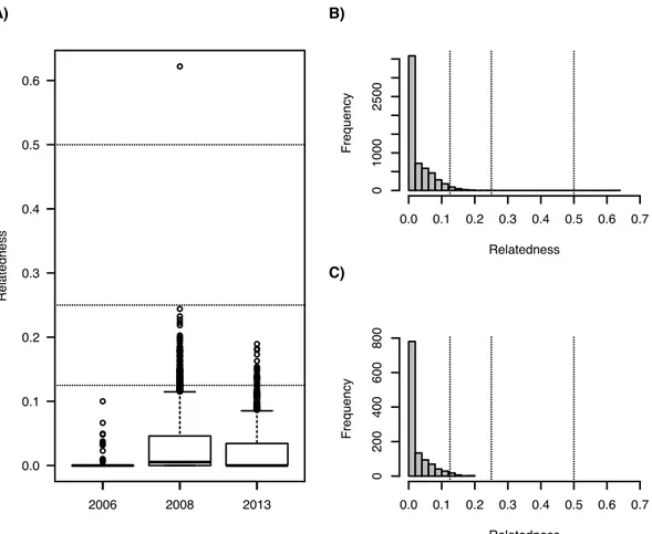
Fig. 2 Pairwise relatedness coefficient estimates among H. guttulatus sampled in
212
2006, 2008 and 2013. Dotted lines highlight a relatedness coefficient of 0.5 (e.g. full 213
sibs or parent-offspring), 0.25 (half-sibs or grandparent-grandchild) and 0.125 (first 214
cousins, aunt/uncle - offspring). A) Pairwise relatedness in each sample. B) 215
Frequency of pairs of individuals distribution in 2008. C) Frequency of pairs of 216
individuals distribution in 2013. Frequency of pairs of individuals distribution in 2006 217
is not shown (N = 13). 218
219
Diversity and relatedness in the Thau lagoon population 220
Monomorphic loci among all individuals or loci with minor allelic frequencies lower 221
than 5% were removed, so that we used 291 SNPs for all 172 individuals, with no 222
missing data. All loci showed heterozygotes in every sample (2006, 2008 and 2013) 223
and genetic diversity remained stable over time (Ar-2006= 1.89, Ar-2008= 1.93 and A
r-224
2013= 1.92; He-2006= 0.336, He-2008= 0.328 and He-2013= 0.326; p-values > 0.99). Note
225
that 13 samples were used to estimate Ar, i.e. a measure of genetic diversity that takes
226
into account variation of sample size. No departure from Hardy-Weinberg equilibrium 227
was observed (FIS-2006 = 0.0001, FIS-2008 = 0.006, FIS-2013= 0.008; p-values > 0.99)
228
along with no temporal genetic differentiation (FST = 0.0001, p-value = 0.91).
229
We estimated relatedness using the assumptions of inbreeding and no inbreeding
230
(Wang 2007) and similar results were obtained. As there was little evidence for
231
inbreeding (see below), we present results with no inbreeding. Relatedness
232
coefficients ranged from 0 to 0.10 in 2006 (mean ± sd = 0.006 ± 0.017), from 0 to
233
0.62 in 2008 (mean ± sd = 0.027 ± 0.038) and from 0 to 0.19 in 2013 (mean ± sd =
234
0.022 ± 0.034; Fig. 2). Relatedness was not significantly different between the three
235 0.0 0.1 0.2 0.3 0.4 0.5 0.6 Relatedness 2006 2008 2013 A) Relatedness Frequency 0.0 0.1 0.2 0.3 0.4 0.5 0.6 0.7 0 1000 2500 B) Relatedness Frequency 0.0 0.1 0.2 0.3 0.4 0.5 0.6 0.7 0 200 400 600 800 C)
study years (p-value = 0.93). Based on simulations, relatedness estimator comparisons
236
between the calculated relatedness coefficient values and the expected relatedness
237
values were not significantly different (expected levels of relatedness r = 0.005, 0.26
238
and 0.21 in 2006, 2008 and 2013, respectively; Wilcoxon signed ranks test, Z =
-239
1.807, p-value = 0.071). Over all dyad comparisons, only one (0.01%) was identified
240
with a relatedness coefficient higher than 0.5, suggesting the presence of
parent-241
offspring or full sibling pairs in 2008 (Fig. 2B). In 2008, most relatedness estimates
242
(97.54 %) of relatedness coefficients values were lower than 0.125 (i.e. first cousins
243
relatedness) while 2.45% ranged from 0.125 to 0.25 (i.e. halfsibs, avuncular,
244
grandparent-grandchild relatedness), suggesting that most dyads remained mostly
245
unrelated. In 2013, a similar pattern was seen with a maximum relatedness estimate of
246
0.189; 97.8% of relatedness coefficients estimates were lower than 0.125 while 2.28%
247
ranged from 0.125 to 0.25. While in 2006, all relatedness estimates were lower than
248 0.125. 249 250 251 252 253 254
Fig. 3 Distributions of observed multi-locus heterozygosity (in gray) and expected
255
multi-locus heterozygosity under random mating (black lines) in 2008 (A) and 2013 256 (B). 257 258 Heterozygosity-Fitness correlations 259
Multi – Locus Heterozygosity (MLH) ranged from 85 to 111 in 2006 (mean ± sd = 98 260
± 8.0), from 77 to 111 in 2008 (mean ± sd = 94 ± 7.7) and from 65 to 110 in 2013 261
(mean ± sd = 93 ± 9.3; Fig. 3, data of 2006 not shown). MLHs were normally 262
distributed (Shapiro test p-values = 0.24, 0.61 and 0.16 in 2006, 2008 and 2013, 263 MLH frequency 0.00 0.02 0.04 0.06 0.08 60 80 100 120
A)
MLH 0.00 0.02 0.04 0.06 0.08 60 80 100 120B)
respectively; Fig. 3, data of 2006 not shown) and no difference in MLH distribution 264
was observed over time (t-test p-value = 0.38). 265
Identity disequilibrium, i.e. a measure of departure from random associations of 266
homozygosity between loci, was only identified in 2013 (g2= 0.003, p-value = 0.015),
267
mainly due to two individuals with low MLH (Fig. 3). This suggests that these 268
individuals may be inbred. No identity disequilibrium remained when removing these 269
two individuals (g2=0.00002, p-value = 0.46). No identity disequilibrium was
270
identified in 2008 (g2=0.0002, p-value = 0.42).
271
Heterozygosity did not correlate with fitness traits, regardless of trait tested 272
(Asymmetry Index estimated in 2008 per individual with its replicate, snout length, 273
total length and weight; p-values on Spearman tests ranged from 0.11 to 0.75). 274
275
Effective population size
276
Temporal changes in allele frequencies estimated Ne per generation (2-year
277
generation time) of 2742 at Thau (Confidence Interval (CI) = (665, +∞)). Larger 278
generation time (3- and 5-year generation time) basically lead to smaller point 279
estimates, but more uncertainties with higher CIs (Ne-3y generation time = 1329, CI=(286,
280
+∞) and Ne-5y. generation time = 1008, CI = (165, +∞)). Smaller values were estimated with
281
single-sample method, with nonetheless overlapping CIs: Nb estimations varied from
282 959 (CI = (796, 1201)) in 2008 to 845 (CI = (601, 1401)) in 2013. 283 284 285 Discussion 286
Indirect study using predictions of population genetics produces particularly 287
valuable information for marine species (Waples 1998). In the present study, genetic 288
diversity of the isolated Thau population of the Mediterranean lagoon ecotype of H. 289
guttulatus proved to remain stable over a seven-year period. We did not identify
290
significant temporal genetic structure, departure from Hardy-Weinberg nor identity 291
equilibrium. Most individuals were likely unrelated and the population mainly 292
outbred, with a unique pair of related individuals identified in 2008, and two inbred 293
individuals in 2013. Heterozygosity did not significantly correlate with fitness traits, 294
reflecting a population with no strong variance in inbreeding, and therefore no 295
evidence of inbreeding depression (Szulkin et al. 2010). All results suggest that the 296
Thau lagoon H. guttulatus population is large and panmictic and therefore will not be 297
affected by the detrimental effects of genetic drift and inbreeding. 298
299
We observed only two inbred individuals in our sample of 172 seahorses. H. 300
guttulatus is usually described sedentary, with low mobility, although it may disperse
301
up to 150m in a single day (Caldwell and Vincent 2012) with home ranges of up to 302
400m2 (Garrick-Maidment et al. 2010). However they are thought to undergo seasonal 303
migrations and have an ontogenic habitat shift. Regarding the inbred crosses found in 304
this study, relatives may have mated because dispersal is not effective or because they 305
dispersed collectively (Broquet et al. 2013; Yearsley et al. 2013). Inbreeding variance 306
was not observed in our samples using identity disequilibrium (g2) and
307
Heterozygosity-Fitness Correlations (HFCs) were not identified. HFCs have been 308
widely examined in natural populations (review in Chapman et al. 2009), although 309
such correlations should only be detected in population with a high variance of 310
inbreeding (Bierne et al. 2000; Szulkin et al. 2010). Our results suggest the study 311
population of seahorse does not seem suffering from inbreeding depression, even if 312
inbreeding could occur in the Thau lagoon. 313
The census size of the Thau population of H. guttulatus is thought to have varied 314
by factors from 1 to 10 over time according to an 8-year SCUBA-diving survey 315
(Louisy and Bérenger 2015). Although protocols were modified throughout the 316
survey, making dives difficult to compare, this monitoring gave an overview of Thau 317
H. guttulatus fluctuations, with a minimum size observed in 2006 following lagoon
318
pollution events, and a maximum in 2009-2010 (Louisy and Bérenger 2015). As 319
expected the effective population size (Ne) remained stable from 2006 to 2013 and
320
reflects the harmonic mean of the census size over that period. Indeed, not all adults 321
effectively reproduce; hence, Ne estimates correspond to the smallest census size of
322
the study time series. Our estimate therefore corresponds to oscillation minima of the 323
population size. Therefore the population of H. guttulatus in this 75 km² lagoon (~50 324
individuals km-2) is likely large enough that demographic events would not impact 325
genetic diversity much, a result in agreement with large scale genetic studies (López 326
et al. 2015; Woodall et al. 2015; Riquet et al. 2019). Such fluctuations in census size 327
population were also observed in the Ria Formosa coastal lagoon (southern Portugal). 328
H. guttulatus declined by 94% over 5 years (Curtis and Vincent 2006; Caldwell and
329
Vincent 2012) due to a combination of habitat loss (Curtis 2007; Gamito 2008; 330
Correia et al. 2015) and coastal ocean warming (Teles-Machado et al. 2007), and is 331
now recovering (Correia et al. 2015). In Galicia, similar effective population size 332
estimates have been obtained (López et al. 2015). Although Ne estimates should be
333
considered with caution (Hare et al. 2011), H. guttulatus Ne estimates are larger than
334
most endangered species (e.g. Chapman et al. 2002; Hoarau et al. 2005), which 335
should ensure the maintenance of genetic variation across the longer term providing 336
appropriate management practices are maintained. 337
338
Seahorses are characterized by a strong parental investment, ensuring 339
reproductive success even at low densities. This was hypothesized to make them more 340
able to endure severe population demographic events such as bottleneck events 341
caused by environmental perturbations for instance, when compared to species with 342
low parental investment (Romiguier et al. 2014). Traill et al. (2010) showed that 343
exceeding the number of individuals required for management and conservation plans 344
will ensure the viability and longevity of the population. In this context, monitoring 345
the Thau population of H. guttulatus over time is important in order to foster the 346
results observed here, especially facing the global warming and other threats they will 347
have to face. 348
Genetic monitoring of this recently discovered conservation unit in H. 349
guttulatus should continue to quantify any temporal changes in population genetic
350
metrics in response to ever-increasing anthropogenic changes to natural ecosystems, 351
which may affect the long-term status of this lineage. Keeping H. guttulatus an 352
ambassador in marine conservation makes sense. Facing alarming statistics regarding 353
marine biodiversity decline and efforts (Hendriks et al. 2006; Lotze et al. 2006), 354
fascinating and iconic marine species, such as H. guttulatus, act efficiently as flagship 355
for other endangered species and ecosystems such as Mediterranean lagoons (Pérez-356 Rufaza et al. 2011). 357 358 Acknowledgment 359
We are very grateful to local citizens, especially fishermen and divers, for their great 360
help in collecting the fin samples used in this work. This work was funded by 361
Languedoc-Roussillon Region “Chercheur(se)s d’avenir" (Connect7 project), by a 362
LabEx CeMEB postdoctoral fellowship to FR, by Chocolaterie Guylian and a Natural 363
Environment Research Council Industrial Case studentship (NER/S/C/2005/13461) to 364
LW, and by a Fondation Nature & Découvertes grant to association Peau-Bleue and 365
PL. This is article 2019-XXX of Institut des Sciences de l’Evolution de Montpellier. 366
367
References
368
Balloux F, Amos W, Coulson T. 2004. Does heterozygosity estimate inbreeding in 369
real populations? Molecular Ecology 13:3021–3031. 370
Bierne N, Tsitrone A, David P. 2000. An inbreeding model of associative 371
overdominance during a population bottleneck. Genetics 155:1981–1990. 372
Broquet T, Viard F, Yearsley JM. 2013. Genetic drift and collective dispersal can 373
result in chaotic genetic patchiness. Evolution 67:1660–1675. 374
Caldwell IR, Vincent ACJ. 2012. A sedentary fish on the move: effects of 375
displacement on long-snouted seahorse (Hippocampus guttulatus Cuvier) 376
movement and habitat use. Environmental Biology of Fishes 96:67–75. 377
Caughley G. 1994. Directions in conservation biology. Journal of animal ecology 378
63:215–244.
379
Chapman RW, Ball AO, Mash LR. 2002. Spatial homogeneity and temporal 380
heterogeneity of red drum (Sciaenops ocellatus) microsatellites: effective 381
population sizes and management implications. Marine Biotechnology 4:589– 382
603. 383
Chapman, J. R., S. Nakagawa, D. W. Coltman, J. Slate, and B. C. Sheldon. 2009. A
384
quantitative review of heterozygosity–fitness correlations in animal
385
populations. Molecular Ecology 18:2746–2765.
386
Claude J. 2008. Morphometrics with R. Springer, New York 387
Correia M, Caldwell IR, Koldewey HJ, Andrade JP, Palma J. 2015. Seahorse 388
(Hippocampinae) population fluctuations in the Ria Formosa Lagoon, south 389
Portugal. Journal of Fish Biology 87:679–690. 390
Curtis JMR. 2007. Validation of a method for estimating realized annual fecundity in 391
a multiple spawner, the long-snouted seahorse (Hippocampus guttulatus), 392
using underwater visual census. Fishery Bulletin 105:327–337. 393
Curtis JMR, Vincent ACJ. 2006. Life history of an unusual marine fish: survival, 394
growth and movement patterns of Hippocampus guttulatus Cuvier 1829. 395
Journal of Fish Biology 68:707–733. 396
David P. 1998. Heterozygosity–fitness correlations: new perspectives on old 397
problems. Heredity 80:531–537. 398
David P, Pujol B, Viard F, Castella V, Goudet J. 2007. Reliable selfing rate estimates 399
from imperfect population genetic data. Molecular Ecology 16:2474–2487. 400
Do C, Waples RS, Peel D, Macbeth GM, Tillett BJ, Ovenden JR. 2014. NeEstimator 401
v2: re-implementation of software for the estimation of contemporary 402
effective population size (Ne) from genetic data. Molecular Ecology 403
Resources 14:209–214. 404
Doyle J, Doyle J. 1987. A rapid DNA isolation procedure for small quantities of fresh 405
leaf tissue. Phytochemical Bulletin 19:11–15. 406
Dryden IL, Mardia KV. (1998). Statistical shape analysis. John Wiley & Sons, Ltd, 407
Chichester. p XIX, 5 408
Foster SJ, Vincent ACJ. 2004. Life history and ecology of seahorses: implications for 409
conservation and management. Journal of Fish Biology 65:1–61. 410
Fraser DJ, Hansen MM, Østergaard S, Tessier N, Legault M, Bernatchez L. 2007. 411
Comparative estimation of effective population sizes and temporal gene flow 412
in two contrasting population systems. Molecular Ecology 16:3866–3889. 413
Frankham R. 1995. Conservation Genetics. Annual Review of Genetics 29:305–327. 414
Frankham R, Bradshaw CJA, Brook BW. 2014. Genetics in conservation 415
management: Revised recommendations for the 50/500 rules, Red List criteria 416
and population viability analyses. Biological Conservation 170:56–63. 417
Gamito S. 2008. Three main stressors acting on the Ria Formosa lagoonal system 418
(Southern Portugal): Physical stress, organic matter pollution and the land– 419
ocean gradient. Estuarine, Coastal and Shelf Science 77:710–720. 420
Garrick-Maidment N, Trewhella S, Hatcher J, Collins KJ, Mallinson JJ. 2010. 421
Seahorse tagging project, Studland Bay, Dorset, UK. Marine Biodiversity 422
Records 3:e73 (4 pages). 423
Gilbert KJ, Whitlock MC. 2015. Evaluating methods for estimating local effective 424
population size with and without migration. Evolution 69:2154-66. 425
Hare MP, Nunney L, Schwartz MK, Ruzzante DE, Burford M, Waples RS, Ruegg K, 426
Palstra F. 2011. Understanding and estimating effective population size for 427
practical application in marine species management. Conservation Biology: 428
The Journal of the Society for Conservation Biology 25:438–449. 429
Hendriks IE, Duarte CM, Heip CHR. 2006. Biodiversity Research Still Grounded. 430
Science 312:1715–1715. 431
Hill WG. 1981. Estimation of effective population size from data on linkage 432
disequilibrium1. Genetic Ressources 38:209–216. 433
Hoarau G, Boon E, Jongma DN, Ferber S, Palsson J, Veer HWV der, Rijnsdorp AD, 434
Stam WT, Olsen JL. 2005. Low effective population size and evidence for 435
inbreeding in an overexploited flatfish, plaice (Pleuronectes platessa L.). 436
Proceedings of the Royal Society of London B: Biological Sciences 272:497– 437
503. 438
Keenan K, McGinnity P, Cross TF, Crozier WW, Prodöhl PA. 2013. diveRsity: An R 439
package for the estimation and exploration of population genetics parameters 440
and their associated errors. Methods Ecology Evolution 4:782–788. 441
López A, Vera M, Planas M, Bouza C. 2015. Conservation genetics of threatened 442
Hippocampus guttulatus in vulnerable habitats in NW Spain: temporal and
443
spatial stability of wild populations with flexible polygamous mating system 444
in captivity. PLoS ONE 10:e0117538. 445
Lotze HK, Lenihan HS, Bourque BJ, Bradbury RH, Cooke RG, Kay MC, Kidwell 446
SM, Kirby MX, Peterson CH, Jackson JBC. 2006. Depletion, degradation, and 447
recovery potential of estuaries and coastal seas. Science 312:1806–1809. 448
Louisy P. and Bérenger L. (2015). Hippocampes et syngnathes du Golfe du Lion : état 449
des connaissances. Association Peau-Bleue - Agence des aires marines 450
protégées, 94 p. 451
Luikart G, Ryman N, Tallmon DA, Schwartz MK, Allendorf FW. 2010. Estimation of 452
census and effective population sizes: the increasing usefulness of DNA-based 453
approaches. Conservation Genetics 11:355–373. 454
Palmer AR. 1994. Fluctuating asymmetry analyses: a primer. Pp. 335–364 in T. A. 455
Markow, ed. Developmental Instability: its Origins and Evolutionary 456
Implications: Proceedings of the International Conference on Developmental 457
Instability: Its Origins and Evolutionary Implications, Tempe, Arizona, 14–15 458
June 1993. Springer Netherlands, Dordrecht. 459
Pérez-Ruzafa A, Marcos C, Pérez-Ruzafa IM. 2011. Mediterranean coastal lagoons in 460
an ecosystem and aquatic resources management context. Physics Chemistry 461
Earth Parts ABC 36:160–166. 462
R Core Team (2017). R: A language and environment for statistical computing. R 463
Foundation for Statistical Computing, Vienna, Austria. URL
https://www.R-464
project.org/. 465
Riquet F, Le Cam S, Fonteneau E, Viard F. 2016. Moderate genetic drift is driven by 466
extreme recruitment events in the invasive mollusk Crepidula fornicata. 467
Heredity 117:42–50. 468
Riquet F, Liautard-‐‑Haag C, Woodall L, Bouza C, Louisy P, Hamer B, Otero-‐‑Ferrer F, 469
Aublanc P, Béduneau V, Briard O, El Ayari T, Hochscheid S, Belkhir K, 470
Arnaud-‐‑Haond S, Gagnaire P-A, Bierne N. 2019. Parallel pattern of 471
differentiation at a genomic island shared between clinal and mosaic hybrid 472
zones in a complex of cryptic seahorse lineages. Evolution 73:817–835. 473
Rohlf FJ. (2010). tpsDig. Stony Brook, NY: Department of Ecology and Evolution, 474
State University of New York. 475
Rohlf FJ, Slice D. 1990. Extensions of the procrustes method for the optimal 476
superimposition of landmarks. Systematic Biology 39:40–59. 477
Romiguier J et al. 2014. Comparative population genomics in animals uncovers the 478
determinants of genetic diversity. Nature 515:261–263. 479
Rousset F. 2008. genepop’007: a complete re-implementation of the genepop 480
software for Windows and Linux. Molecular Ecology Resources 8:103–106. 481
Roux C, Fraïsse C, Romiguier J, Anciaux Y, Galtier N, Bierne N. 2016. Shedding 482
light on the grey zone of speciation along a continuum of genomic divergence. 483
PLOS Biology 14:e2000234. 484
Slate J, David P, Dodds KG, Veenvliet BA, Glass BC, Broad TE, McEwan JC. 2004. 485
Understanding the relationship between the inbreeding coefficient and 486
multilocus heterozygosity: theoretical expectations and empirical data. 487
Heredity 93:255–265. 488
Spearman C. 1904. “General intelligence,” objectively determined and measured. 489
American Journal of Psychology, 15: 201–292. 490
Szulkin M, Bierne N, David P. 2010. Heterozygosity-Fitness Correlations: A time for 491
reappraisal. Evolution 64:1202–1217. 492
Teles-Machado A, Peliz Á, Dubert J, Sánchez RF. 2007. On the onset of the Gulf of 493
Cadiz Coastal countercurrent. Geophysical Research Letters 34:L12601. 494
Traill LW, Brook BW, Frankham RR, Bradshaw CJA. 2010. Pragmatic population 495
viability targets in a rapidly changing world. Biological Conservation 143:28– 496
34. 497
Wang J. 2001. A pseudo-likelihood method for estimating effective population size 498
from temporally spaced samples. Genetic Ressources 78:243–257. 499
Wang J. 2007. Triadic IBD coefficients and applications to estimating pairwise 500
relatedness. Genetics Research 89:135–153. 501
Wang J, Whitlock MC. 2003. Estimating effective population size and migration rates 502
from genetic samples over space and time. Genetics 163:429–446. 503
Waples RS. 1989. A generalized approach for estimating effective population size 504
from temporal changes in allele frequency. Genetics 121:379–391. 505
Waples RS (1998) Separating the wheat from the chaff: Patterns of genetic
506
differentiation in high gene flow species. Journal of Heredity. 89: 438–450.
507
Waples RS. 2005. Genetic estimates of contemporary effective population size: to 508
what time periods do the estimates apply? Molecular Ecology 14:3335–3352. 509
Waples RS. 2006. Seed banks, salmon, and sleeping genes: effective population size 510
in semelparous, age-structured species with fluctuating abundance. The 511
American Naturalist 167:118–135. 512
Waples RS, Do C. 2008. ldne: a program for estimating effective population size from 513
data on linkage disequilibrium. Molecular Ecology Resources 8:753–756. 514
Waples RS, Do C. 2010. Linkage disequilibrium estimates of contemporary Ne using 515
highly variable genetic markers: a largely untapped resource for applied 516
conservation and evolution. Evolutionary Applications 3:244–262. 517
Wilks SS. 1932. Certain generalizations in the analysis of variance, Biometrika, 24: 518
471-494. 519
Woodall LC, Jones R, Zimmerman B, Guillaume S, Stubbington T, Shaw P, 520
Koldewey HJ. 2012. Partial fin-clipping as an effective tool for tissue 521
sampling seahorses, Hippocampus spp. Journal of the Marine Biological 522
Association of the United Kingdom 92:1427–1432. 523
Woodall LC, Koldewey HJ, Boehm JT, Shaw PW. 2015. Past and present drivers of 524
population structure in a small coastal fish, the European long snouted 525
seahorse Hippocampus guttulatus. Conservation Genetics:1–15. 526
Yearsley JM, Viard F, Broquet T. 2013. The effect of collective dispersal on the 527
genetic structure of a subdivided population. Evolution 67:1649–1659. 528