Determination of directional spectra of sea surface wave field by scanning observation.

DETERMINATION OF DIRECTIONAL SPECTRA OF SEA SURFACE WAVE FIELD

BY SCANNING OBSERVATION

by

Piotr Koziol

Warsaw University, Poland 1971

SUBMITTED IN PARTIAL FULFILLMENT OF THE REQUIREMENTS FOR THE DEGREE OF

MASTER OF SCIENCE at the

MASSACHUSETTS INSTITUTE OF TECHNOLOGY

11 May 1972

Signature of Author...'...

Department of Meteor gy, 11 May 1972

Certified by ... .. ... Thesis Supervisor Accepted by... ... ... ...

am

da~~ruttmental Committee on ua .dents

SI~sj 1972

DETERMINATION OF DIRECTIONAL SPECTRA OF SEA SURFACE WAVE FIELD

BY SCANNING OBSERVATION

by

Piotr Koziol

Submitted to the Department of Meteorology on 11 May 1972 in partial fulfillment of the requirement for the

degree of Master of Science

ABSTRACT

This paper considers the possibility of determining the direc-tional energy spectrum of ocean surface gravity waves from a set of one-dimensional spectra. The one-dimensional spectra are in Doppler shifted frequency domain and they are obtained from the signal given by towing a measuring device in different directions across a wave field. An attempt to solve the integral equation involved approxima-ting it by a set of simultaneous linear algebraic equations led to a singular matrix.

Thesis Supervisor: Erik Mollo-Christensen Title: Professor of Meteorology

TABLE OF CONTENTS 1. INTRODUCTION 4 2. THEORY 5 3. EXPERIMENT 14 A. Data Collection 14 B. Data Analysis 14

4. RESULTS AND DISCUSSION 27

5. SUGGESTIONS 29

6. ACKNOWLEDGEMENTS 31

LIST OF FIGURES

Fig. 2A Surfaces Sd and S 7

Fig. 2B Projection of Snf S on k plane 7

Fig. 2C k and (k,y) spaces 12

Fig. 3A Spectrum of the FM signal 18 Figs. 3B (1-6) Spectra in Doppler shifted frequency 19-24

domain

Fig. 4A £jth projection of SgAS on k plane 28

1. INTRODUCTION

The knowledge about the directional energy spectrum of a wave field is of interest in many applied sciences. In the case of

ocean surface gravity waves, one of the possible methods is measure-ments of a sea surface elevation at a set of points on the sea and

then (assuming stationarity and homogeneity of the wave field), using the time correlation analysis of data, one can get some information about the directional spectrum. The results depend strongly on the spatial distribution of wave detectors. One can optimize their

rela-tive positions with respect to the studied wave phenomenon. Still, the directional resolving power of the optimum array is limited. In this paper, a possibility of determining the directional spectrum from a set of one-dimensional spectra (as opposed to the co-spectra method mentioned above) is considered.

One can avoid the difficulties caused by measurements at dis-crete points or at disdis-crete times by a continuous observation of water elevation in time and in space. A measuring device in this case moves with a known velocity across the wave field. As a result, a one-dimen-sional spectrum in a Doppler shifted frequency domain is obtained. This time waves with different wavenumbers, frequencies and directions of propagation contribute to a value of energy corresponding to a given Doppler shifted frequency. By towing the measuring device in different directions and with several values of velocity, one can collect enough information to deduce the directional distribution of energy.

2. THEORY

The directional energy spectrum is, in general, a third order

density: i (in)

where k is the wavenumber vector and a is the frequency. If the measuring device moves with a velocity U, the signal obtained has

the following spectrum:

where S- is the surface consisting of the points (k,a) that give the same value of a Doppler shifted frequency, the argument of the left-hand side. Because we cannot distinguish between positive and nega-tive values of frequency, the equation of this surface is:

U

and

is the measured one-dimensional spectrum.

If we now assume a dispersion relationship between k and o, the equation of the corresponding surface, valid for deep water gra-vity waves, is:

It implies that

i.e. the energy lies on the dispersion relationship surface S and (k) is the directional spectrum we are looking for.

The measured spectrum becomes:

(2.1)

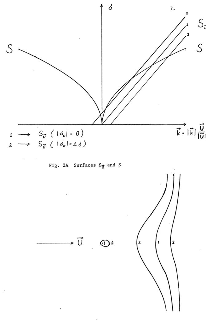
where Sj1C S is a projection of an intersection of the surfaces S-, and

S on the k plane (Figs. 2A, 2B). Therefore, ( j) is now equal to a second order density Y(k) integrated over a line Si S.

In order to solve the integral equation (2.1) for T, we can try approximating it with a set of simultaneous equations, i.e. we have to change the description of the problem from a continuous to a discrete

one. In this approach, the data

(Iyo

I)

becomes the right-hand side

/,2

r

u

Fig. 2A Surfaces S# and S

---

~U

<

~2

Fig. 2B Projection of S,-n S on k plane

5

I I~-~-~-*I

L-YL*IC ..

~L

-L1-l~-l*~-

-II.--~LY_

vector, the distribution of energy T becomes the unknown vector and the integral operator

Jf

becomes the matrix that is determined by the geometry of the problem, i.e. by surfaces S# and S.

It is now convenient to change the coordinates from cartesian to polar

In the discrete description, we have to specify a size of k space; in other words, we expect Y(k)

#

0 for

Ikj

< K. Then the maximum value of Doppler shifted frequency can be related to K by:

Also, the data must be smoothed over some interval Ao, and then the right-hand side values should be taken at points

Iool

= integer • Au.

Concommitantly, one has to replace the densities of nth order by the products:

density

(

Xe

Z

-

x;

Let us determine Au as:

a

/i(id

0

I_

)=ILIK

where

IAUI

is the accuracy within which we can measure and maintain the velocity of the device.

Having specified the size of k space in which we are looking for energy distribution, we should fill it in with points. Their number has to be smaller than the amount of the right-hand side values, which for one graph (aI) is given by:

16o]+

-

+I

If one plans to use polar coordinates, the angle interval Ay should be larger than the accuracy within which one can determine the direc-tion the device moves:

Now the values of Ay, K andl a Imax specify the size of Ak which is the wavenumber interval. Ak should satisfy:

2rn

4k ITF

of

Now there is a possibility

parameters by comparing AG

A

(Vk

k-K

to check the orders of magnitude of all the with:

F5

Ak

2

10.

The next step is to write down the set of simultaneous equa-tions that corresponds to the integral equation (2.1). At first, one has to index all the points in k space, i.e. to a given pair

(kuy>

(Ar

ak)

( M )

,,r

we relate a subscript Z, so the values of energy

e

consist of the unknown vector (dimension [Z ] = cm2). Each value from the graphs (GODi) becomes a component of the right-hand side vector.

kjth value ( 1 < < n+l) on the jth graph (corresponding to velocity Uj) has a subscript

and we write it as Vp:

(dimension [Vp] = cm2).

The amount of experiments (number of different U) should assure the condition

11.

and we will use the first Pmax of the Pmax equations. The pth equation is of the form

j 1.

A

(2.2)

where 1 < p <

kmax

and the matrix element is equal to zero if a given point in k space does not contribute to the right-hand side value and is equal to one if it does. We define functions:

&

EL 3 + UeYk Cs c M()d')

=

-

(Ii-

1

)

6

+

U,(() A k

f,,s(Wj-y,()4)

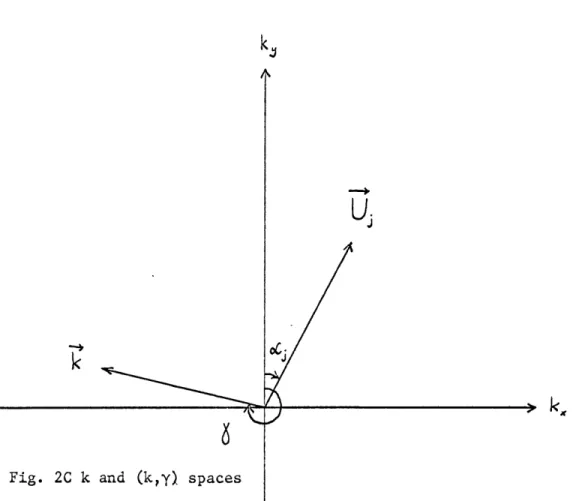
where (Fig. 2C) :

and

j

= integer part (P-) + 1

jt = p - (n+l)(j-l)

IUi

LU

]O~;nil,

_I~L~li_ _^IX_ *__IIL _*_IUIII-UI~ Il~l~-^LI -i--i__-I^~X~~_

b

sS-~1~

V F

Fig. 2C k and (k,y) spaces

12.

Ui

13.

Then we find the matrix as follows:

1

e)

--14.

3. EXPERIMENT AND INSTRUMENTS

A. Data Collection

The experiment took place at Quincy Bay on the sixth of April

1972 at six p.m. The wind was blowing from the South and its

velo-city was seven knots.

The experiment consisted of towing a wavegauge from a two-meter bowsprit mounted on the boat. The magnitude of ship velocity was

kept constant (800 R.P.M. = 228 cm sec- ) and data were recorded for

different directions of scanning. An FM signal from the wavegauge

was recorded on a closed-loop (time of one loop = 1 min 53 sec) by an eight channel tape recorder. A different channel was used to

record the data from each direction of scanning.

The process of recording of one tape took less than twenty

minutes. One had to select the optimum compromise between the length of a closed-loop (the longer it is, the better the quality of spectrum

obtained) and the total time of the experiment. (It should not be too

long if the data from different directions are to represent the same wave field).

B. Data Analysis

From the recorded signal, we want to obtain the energy density cm2

averaged over a frequency interval AG (dimension = HZ-). The FM signal was converted to a voltage signal which was played back one

hundred times faster than it was recorded. The signal was next passed

15.

through a QUAN-TECH wave analyzer, which gave as an output ampli-tude versus frequency. The parameters of the QUAN-TECH wave analyzer were as follows: Sweep width = SW = 5 kHz

Band Width = BW = 10 Hz Averaging time = TC = 10 sec

Sec

The Sweep time = ST = 1800Ywas chosen to be much larger than the time 1 min 53 sec

of one closed-loop cycle = 100 in order to obtain a consis-tent spectrum. Additionally, all these parameters had to satisfy the relationship required by the properties of the wave analyzer:

1

4sw

BW

eyro

ST

(BW)

where error was assumed to be = 2%.

The spectrc, obtained in this way have a long "tail" (that comes from a circuit noise) of an almost constant level. Having subtracted the noise level, one can determine the order of magnitude of

IDI

max which

is > 2f * 30 Hz. We solve next for K to satisfy:

r---I&

I

,

+

UK

and for U = 228 cm sec- one finds K =.75cm- 1 . Assuming 3% accuracy in determining the value of U, one computes AGo AAlGDmax = AU * K~ 2T * .75 Hz. The next step is to smooth the graphs over the chosen value of the interval AG. We need the values of energy at a discrete

16.

set of points I1DI = integer * Ao. One graph gives us

i

I

i

A c3

n

+1

i

3

Vlodve

so now we define

=

21T7-

31.5

HZ

The wave analyzer output is the amplitude and we need the values of energy, so one has to square the values of amplitude

for J = l,...,n + 1 to obtain

j corresponds to one velocity Uj of the ship. The value of j at

IDI

= O0 is smoothed over Ac/2 and values for IoDI > 0 are smoothed over an

interval Ao. Because all the graphs represent the same wave field, the energy content should be the same for all of them, i.e.:

2

₁₊

qll~lb~l;.

4J

(I

l.

(-j

= _{const (independent of j)}

17.

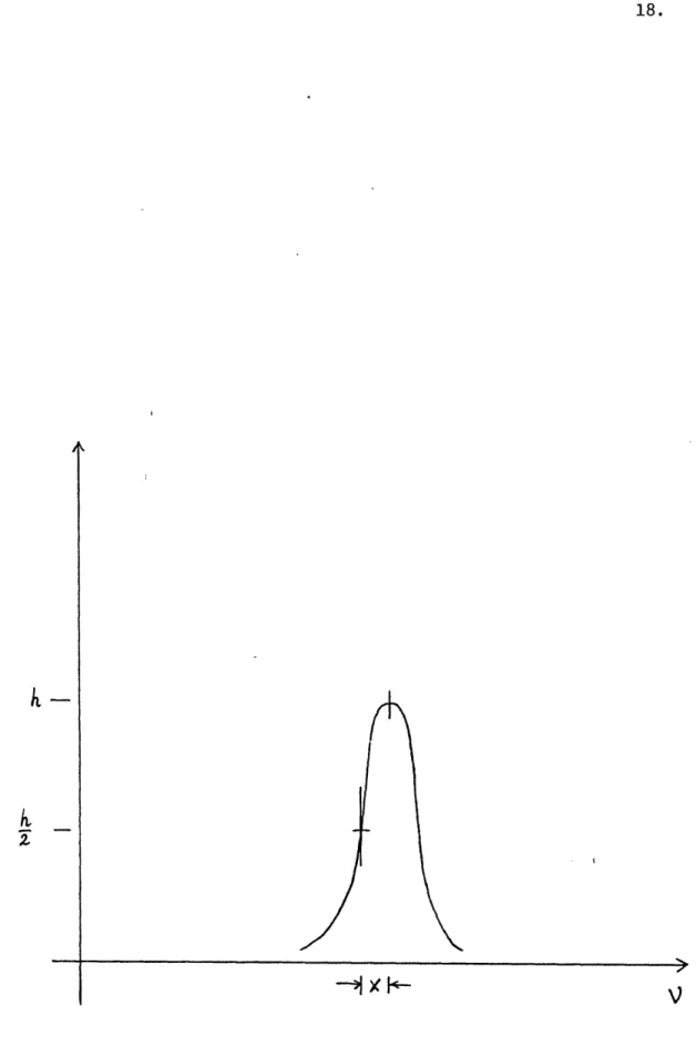
This constant can be found by considering the spectra of the FM signal that are very similar to a normal distribution. Measuring the width at h/2 (Fig. 3A), one can determine the square root of the variance of the FM signal = x - 25.84 Hz (where 7is

2 n 2 the average over all the experiments).

From the calibration of the wave gauge,

= .36

+

Const

(where r - elevation in cm

V - FM frequency in Hz)

one can then specify the energy content in the wave field:

2

8'o.5

c'Q

(mean square amplitude .

Now we are able to scale

2

= 9.3 cm)

the graphs:

J = const = 86.5 cm2 AUT

Scaled .values are represented by Figs. 3B (1-6).

18.

Fig. 3A Spectrum of the FM signal

19. Fig. 3B (1) 6,- e

I6)1

0

Cnm Hz

150

I__lr~l~

Ij

_i~l

IIII

~_L*IIIL)____Y__l

~-_P~RI ~~I*I-

I

20. Fig. 3B (2)

06

=

30

IdJ

10

Hz

CAMS_2s.

Hz

150

100

21. Fig. 3B (3) Cl3

1

D

In

H1

.

i7

I n

Hxz

Hz

150-

100o-

50-O

135"

-C

22. Fig. 3B (4)

6

=

180

It

141

cm Hz

1.50.

lo00

50o

23. Fig. 3B (5)

Z = 225"

10

2. Hz

150

100

50

.24. Fig. 3B (6)

Z

=

3150

2. loo

50

25.

They give the right-hand side values Vp for the set of equations (2.2). In order to find the elements of the matrix Apo, one has to pick a value for Ak. The accuracy in determining and maintaining

the direction of ship velocity was assumed to be

IAc.[

- 40 - .07 radian, so Ay has to be larger than 40. Let us take for Ay a value 22.50,

i.e. we have in the discrete space (k,y) 16 directions. Now Ak can be specified by considering the inequality:

0

<

(L + n u m b e r of

'6

0

)

k

experiments

So we should have:

43-G

Let us take Ak = .05 cm-1, so we have 15 + 1 different values of the magnitude of the wavenumber vector (.0, .05,...,.75). The total number of points in (k,y) space is now equal to:

Ymax = 16 * 15 + 1 = 241

The matrix of the coefficients of the set of simultaneous equa-tions was found by a computer. A column Z of the matrix Apt corresponds to a point in (k,y) space and row p corresponds to the £jth value of C on the jth graph. For a given pair of integers p,Z (1 < p, < 2max = 241)

the computer checks the values of differences:

and () -

(

)

26.

and if at least one of them is less than Aa/2, an adequate matrix element Apt is assigned a value 1; otherwise the value of Apt is 0. This method is equivalent to expressing the lines S-n S on k plane by using the discrete points (k,y); the matrix element is 1 if a given point belongs to a set in the discrete (k,y) space that

re-presents the 7th line S-l S (it means the line corresponding to the jth value of velocity and IGDI = (J3-i)Aa) and if it does not belong,

27.

4. RESULTS AND DISCUSSION

The matrix AL was found to be singular. Let us consider once more the way the matrix was constructed. Two adjacent sets

of lines, S#n S, where:

J

U. and

correspond to two consecutive values of Lj. This means that the re-presentation of the line S

aS

in the discrete (k,y) space is for

J = integer given by all the points which are in the area between the lines ij - 1/2, LJ + 1/2. These are the dotted lines on Fig. 4A

(little arrows show the directions corresponding to the increasing values of iJ). It implies that for a chosen velocity Uj, each point

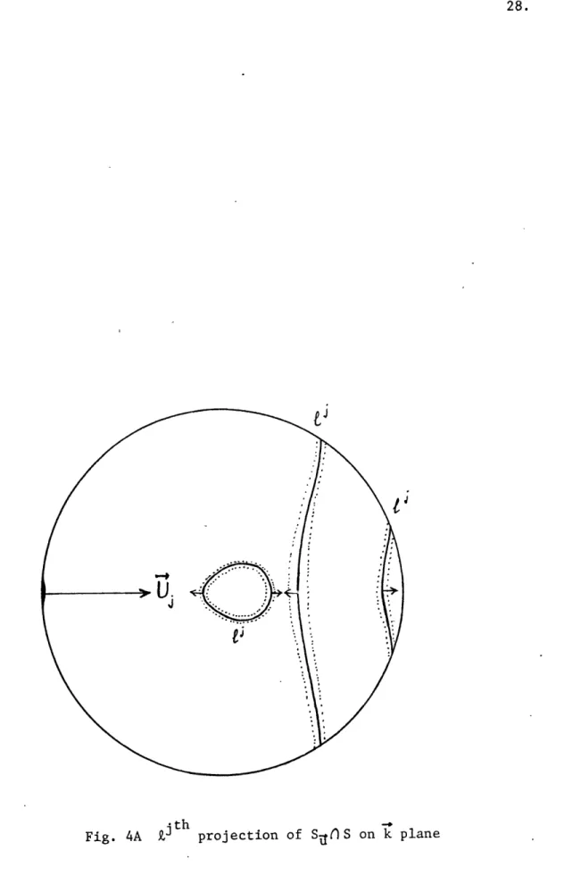
in (k,y) space is used for such a representation exactly once. One point corresponds to one column of the matrix. Consequently, if we add all the rows that are computed for the same Uj (for a given Uj there are 43 of 'them) we will get a row that consists entirely of ones. The same can be obtained by adding rows corresponding to any other velocity Uj. This is one reason why the matrix is singular.

There is another cause of singularity. For a given distribution of points in (k,y) space, one can end up with rows which consist only of zeros. It happens with the Zjth row when the area between the lines

aJ

- 1/2 and J + 1/2 (the dotted lines on Fig. 4A) does not contain

any of the points.

28.

Fig. 4A Zjth projection of S- S on k plane

29.

5. SUGGESTIONS

Let us look once more at the equation (2.1):

What we can get from an experiment are the values of

(IGDI).

The

accuracy within which one can determine the velocity of the ship U as well as the accuracy of the wave analyzer limit the number of right-hand side values (the spectra obtained for the too-close di-rections of U can differ more because of the inaccuracy of the wave analyzer than because of the physics involved), in other words limit the amount of information we start with to some set of values of (a D )(say to m different values).

If we want then to determine a continuous distribution of energy, that is to say the integrand

Y(k),

we can assume a series representa-tion of

Y(k)

with constant coefficients. Next one can proceed to

integrate over S-n S. As a result, the left-hand side of (2.1) becomes a known function of the coefficients mentioned above. The values of

(IaDI)

can then be used to determine the best fit of these parameters to the observations.

In other words, we replace the integral equation (2.1) by a set of linear equations. This time the number of coefficients we are to specify should be smaller than the number of equations (2.1)(=m). Then

30.

one picks the best values for the unknown parameters in terms of minimizing the distance in an m - dimensional space.

31.

ACKNOWLEDGEMENTS

I would like to express my thanks and sincere appreciation to Prof. Erik Mollo-Christensen for his help and interest as well as for our discussions resulting from this project. Thanks are also due to Charlie Flagg and Terry Burch for their encouragement and suggestions. I would also like to give thanks to Miss Trudi Noehren who typed the manuscript.

The author's work and research for this project was supported by a grant from the National Science Foundation.