Designing performative surfaces : computational interpretation of flow pattern drawings

(1)

Designing Performative Surfaces

Computational Interpretation of Flow Pattern Drawings

by

Masoud Akbarzadeh

M. Arch Massachusetts Institute of Technology 2011

M. Sc. in Earthquake and Dynamics of Structures, Iran University of Science and Technology, 2007 B. Sc. in Civil and Environmental Engineering, Zanjan University 2004

Master of Science in Architecture Studies

at the

Massachusetts Institute of Technology

June 2012

@2012

Masoud Akbarzadeh, All rights reserved.

The author hereby grants to MIT permission to reproduce

and to distribute publicly paper and electronic versions

of this thesis document in whole or in part.

Signature of Author:

Certified by:

Accepted by:

JUN

0 8 2012

I RA

I

Department of Architecture May 24, 2012

I1/

Takehiko Nagakura Associate Professor, Massachusetts Institute of Technology

Thac-i

Advisor

Takehiko Nagakura Associate Professor, Massachusetts Institute of Technology Chair of the Department Committee on Graduate Students

(2)

Dennis Shelden Associate Professor, Massachusetts Institute of Technology Thesis Reader

Joel Lamere

Lecturer, Massachusetts Institute of Technology

(3)

(4)

(5)

Computational Interpretation of Flow Pattern Drawings

Acknowledgment

I am thankful to:

Takehiko Nagakura, for his great comments and support at the beginning and through the whole process of this research, Dennis Shelden, For his gener-ous helps and comments on generalizing the mathematical grammar for the research, Joel Lamere, for his important suggestions to frame the research in the boundaries of design. I am also thankful to his generosity to use the tool developed in this thesis for a design purpose and sharing the final re-sult as a design instance, a representative of a complex geometry generated

by the tool, Paul Kassabian, for his great structural consultation throughout

the research, Morteza Zadimoghaddam, for his great help clarifying some computer science related algorithms to be used in this research, Onur Gun, for his great comments on simplification of ideas presented in this research, Alan Tai, for his great helps on developing some of the algorithms in this research, William 0' Brien Jr, for his great design related suggestions, and Ksenia, for her generosity, support and patience throughout the process of this research.

p 5

(6)

Designing Performative Surfaces

1. Introduction

8 1.1 Motivation

1.2 On geometry and Architecture

1.3 Surface representation

1.4 Problem Statement

2. Methodology

₁₄

2.1 Introduction

2.2 Surface Data Structure Background

2.3 Regenerating Surface using Surface Network Graph

2.4 Properties of Surface Network Module

2.5 per-formative Surface Generative Algorithms

3. Surface Data Structures

19 3.1 Introduction

3.1.1 Surface Definition: History

3.1.2. Surface Definition: Mathematical Representation

3.2 Surface Network Extraction Methods

3.2.1 Bilinear Surface Patches Algorithm

3.3. Regenerating Surface Using Surface Network Graphs

3.3.1. Contour extraction

3.3.2. Contour regeneration

3.3.3. Topography Resolution

3.4. Summary

4. Generating Performative Surfaces

38 4.1. Introduction

4.2. Performative Aggregation of Critical Graph

4.3. Surface Generative Algorithm Version 1.

4.4. Surface Generative Algorithm Version 2.

4.5. Surface Generative Algorithm Version 3.

4.5.1. Rationalized drainage direction of a surface

4.5.2. Algorithm Description

4.5.3. Global Drainage

4.5.4. Point Grid Pre-Transformation

4.5.5. Non-linear Transformation of height

4.6. Summary

5- Conclusions

68 6- References

70 P

(7)

Chapter One: Introduction

p 7

(8)

1.1 Motivation

Figure. 1.0. Arthur David

How-ard, Drainage Analysis in

Geo-logic Interpretation A Summation Howard 1967].

In spring 2011, while I was working on my thesis in architectural Design degree, I came across with an interesting problem in design: a parametric river. I realized that it is not possible to control the river parameters without understanding the geometry of the surface of terrain. in other words, the shape of the terrain or topography may change the shape of the river down the hills. I started to look up more examples in geoscience and

geomor-phology to find out more about this topic. I came across drainage patterns which vary based on the shape of the terrain in different parts of the world

[Howard 1967].

As a designer, the first thought passed through my mind was: "is it possible to design a terrain using drainage patterns?! There must be a way to derive the landscape geometry from the one of the the river!" Later on, through searching related topics in geoscience, I realized that this topic has interest-ed researchers from 1858 and there is a quite enormous body of research on that in geo-computation and geography and computer science.

I made this topic as the main goal of present thesis to explore the design

possibility of such representation in architecture and connecting the world of design with hydrological and geological characteristics of the land (Fig.

1.0).

Recently the design proposals tend to become more engaged in sustainabil-ity aspects, more recently in energy generation. Therefore, many designers now seek approaches to integrate architectural ideas with interdisciplinary subjects to tackle the different aspects of energy constrains and sustainabil-ity issues. There is a recently developed area of research among architects which tries to define the design through the lenses of energy production. This field has received more attention in landscape design and planning strategies. Among all energy generating methods such as wind and solar, there are no many examples of addressing the design through hydropower energy generation which is the main basis of investigation in current study. In order to explain the goals of the thesis it is important to clarify the objec-tives of this study in a simple question: Is it possible to construct complex geometry of the surface of the terrain using drainage analysis? Or is it pos-sible to embed required information of 3-dimentional space into 2-dimen-sional drawing. In that case, designers can design complex geometries using simple plan drawings which might result in more function-oriented design.

p 8

(9)

1.2 On Geometry and Architecture

"Geometry is one subject, architecture another, but there is geometry in ar-chitecture. Its presence is assumed much as the presence of mathematics in physics, or letters in words. Geometry is understood to be a constitutive part of architecture, indispensable to it, but not dependent on it in any way. The elements of geometry are thus conceived as comparable to the bricks that make a house, which are reliably manufactured elsewhere and delivered to site ready for use. Architects do not produce geometry, they consume it. Robin Evans, 'The Projective cast' [Evans 1995]

Before any step forward in geometric exploration , it is quintessential to step back and realize the relationship between geometry and architecture through the history of architecture. If I want to define the place of ge-ometry with respect to architecture, I should say gege-ometry is completely independent from architecture. It is a rational science which is manufac-tured somewhere else and consumed by architects. Geometry is a rational science, whereas architecture is a kind of art which is produced and judged

by intuition. In other word, geometry gives architecture a rational

founda-tion to start, but it does not limit it to pure rafounda-tionality.

The first place anyone searches geometry in architecture is in the shape of the buildings. What establishes the shape of the building in our percep-tion is its projecpercep-tion into our eyes. Projecpercep-tion is the process of producing an image of an object on a planar surface. Projection extensively exists in architectural drawings or representations.

Generally, there are two types of projections in drawings: parallel and cen-tral (conical). What is in common for both is that both using lines of sight to project the object onto the projection plane. The difference is that in

parallel projection the lines are parallel, whereas in conical projection they converge to the point of view (focal point). (Fig. 1.1.)

Normal orthographic projection of an object is a branch of parallel projec-tion which we use in everyday design tasks, called plan, secprojec-tion, and eleva-tion. In order to describe the object fully in three dimensions, three projec-tion planes are required, perpendicular on each other. Obviously, this is the reason for having at least three projection planes. Previous to computers, all these representations have been done, in an analogue style, on paper and presented two dimensionally as well. Preserving the same concept, computers revolutionized this approach and presentation styles.

p

(10)

I

Figure 1.1. a. Conical Projection b. parallel projection

a. b.

Advance in computer graphics and visualization allows modelers to design and represent highly complicated geometrical models. Lots of these ge-ometries are regular gege-ometries that can be articulated in computer easily using conventional techniques. But there are many other irregular shapes of practical important to us which cannot be represented easily. For example, topography of the earth is one. How do we represent the properties of such complex geometries? This is a desired subject for researchers in different disciplines including geometers, geographers, computer scientist and even architects! (Fig. 1.2.)

Figure 1.2. surface geom-etry of the Earth, dendritic drainage pattern [A].

p 10

(11)

1.3 Surface Representation

Since current research is intended for designers and architects, Lets have a look at main different methods of surface construction and representa-tion in different disciplines from design point of view. This overview helps

us understand the characteristics of each method and its potentials and drawbacks in terms of design.

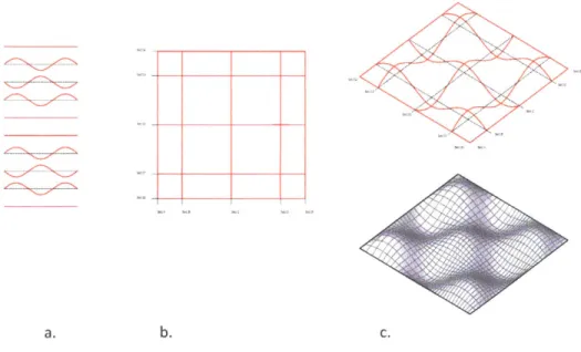
1.3.1 Interpolation of Sectional Curves

In this technique, surface is constructed using multiple sections in two main directions of u, v or s, t. This is the main principle used in constructing con-tinuous surfaces in NURBS' modeling softwares. The main advantage of this technique is generation of precise and manipulatable surfaces in section. The disadvantage of this technique is poor control in plan as well as large number of required sectional curves in constructing complex surfaces. (Fig.

1.3.)

Figure 1.3. Interpolation of Se-tional Curves. a. Design curves /

Required curves to start. b. Plan location of each sectional curve. c. Interpolated result/ Surface of

the curves. a. b. c.

1.3.2. Contour Manipulations

In this technique, designer is obliged to draw the contour representation of the final surface on plan. Contour lines are basically intersection lines between the final surface and parallel planes with specific intervals from defined origin. The advantage of this method is a good control for designers in plan. The disadvantages of this method are: poorly manageable features in section, required time and effort to draw all the contours to represent

and construct a complete surface. (Fig. 1.4.) p

11

(12)

Figure 1.4. Contour manipulation

--a. design requirement elements. b. plan representation of con-toured based desgn. c. Surface result of the contour drawn plan

a.

b.

c.

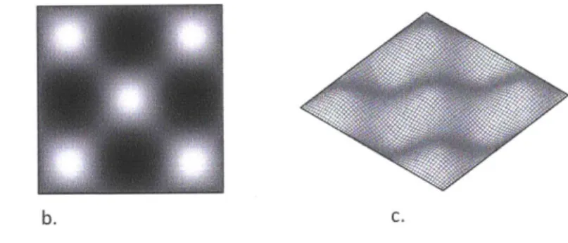
1.3.3. Digital Elevation Model

Digital Elevation Model (DEM) is a technique in surface reconstruction

which uses pixel properties of an images. This method is highly interested

for Geographers and geo-computationalist. The color of each pixel, which

changes in a range from back to white, is translated to the height and

con-sequently the surface is generated using height information of each pixel.

The main advantage of this method is surface generation of image

repre-sentation. The main disadvantage of this technique is the difficult control of

surface behavior in plan and section (Fig. 1.5.)

Figure 1.5. Digital Elevation Model representation of a surface. a. Design elements as pixels and their colors. b. Image representation of surface as

pixels rangnig from bacl to white. _b _c

c. Surface result of elevation data '

1.3.4. Triangulation

Computer graphists use triangulation! extensively in design and

represen-taion. It is a very powerful technique in constructing complex geometries.

This method translate geometry to collection of vertices and creates

triangles from them. The advantage of this method is the possibility of

representing very complex geometries using simple triangles, whereas, the

disadvantages are the enormous amount of time required to design a

ge-p

ometry and poor global manipulation of the complex geometries. (Fig. 1.6.)

12

i The triangulation is named after Boris Delaunay for his work on this topic from 1934.

(13)

Computational interpretation of Flow Pattern Drawings

Figure 1.6. Triangulation. a. Vertices and their corresponding triangles. b. Plan representa-tion of triangulated vertices. c. Mesh Surface Representation of triangles.

a.

2 IA 71 ~ 2

b.

C. 1.4. Problem Statement

As I referred to geomophological drawings of the surface of the earth, there is a conventional method of drawings in geomorphology which represents different complex surface geometries of the earth. now that we revisited

main surface design and representation methods in different disciplies, it is the time to restate the problem for the currnt research:

Is it possible to design and construct complex surface geometries using only plan drawings? in Other word, is it possible to use the drainage pattern of a surface to reconstruct its geometry?

The main intention of this research is to answer this question from design-ers' point of view and provide them a tool for desging such surfaces using only plan drawings. (Fig. 1.7)

Figure. 1.7. Plan drawings of a drainage patern

p 13

V

(14)

---Designing Performative Surfaces

Chapter Two: Methodology

P

14

(15)

2.1. Introduction

The main outcome of this research is a tool and its relevant algorithm for designers to design and generate complex geometries using only plan drawings.(Fig. 2.1.) The algorithm to generate this tool has been achieved through series of surface generation processes using the idea of simple plan drawings. In order to conduct the research, author takes the following steps.

a.

b.

Figure. 2.1. Performative surface

algorithms. a. Algorithm 1. b.

Algorithm 2. c. Algorithm 3.

c.

2.2. Surface data structure background

The main idea of this step is to reduce the whole information of a surface into a graph consoting of points and lines. This will simplify the explana-tion of any complex surface topography into a simple graph representaexplana-tion. (Fig.2.2)

Initially, author starts with the definition of surface data structure, histori-cally [Cayley 1859, Maxwell 1870] and mathematihistori-cally [Morse 1965] . In Mathematics, Surafce data structure is called Critical graph which is a basis for surface networks topic in geo-computation. Respectively, the geo-com-putational methods for extraction of surface network graph from a given geometry or topography is used to understand the behavior of different

surface geometries. [Pfaltz 1976, Schneider. B. and Jo wood 2004]. p

(16)

Assumptions

- In surface network extraction, Each surface or topography is a continuous function, z=f(x,y). There is no whole or under cut in the geometry of the assumed surface

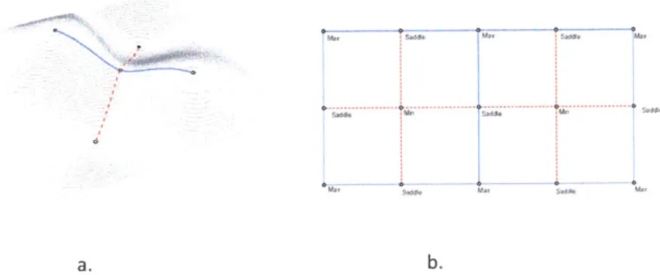
- Extraction of surface network graph is based on bilinear surface patches Surface structure extraction

Figure 2.2. a. Critical Graph consisting of maximum, minimum and saddle points and the lines connecting these points toeachother. b. simplified version of critical graph

2.3. Regenerating Surface using Surface Network Graph

The importance of this step is to learn to construction or regeneration of different types of surface geometry using simple surface network graph concept. The general graph of surface networks is used as a basis to regen-erate different surface geometries. In this step algorithm to extract contours from graphs is provided.(Fig. 2.3)

Assumptions

- There are different types of surface network graphs in geo-computation. The graph that has been used in this step is based on the simple connec-tion between maximum points to pass points, and pass points to minimum points of a surface.

- In this study contours are generated

from

the graph. An algorithm to orga-nize and connect the contours provided by the author

- A secondary algorithm also provided to reshape the contours and regener-ating multiple surfaces from a single surface network graph

p 16

a.

-

_

-

- -

-

--

-

.

(17)

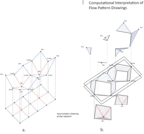
Figure 2.3. a. Surface Netwrok Graph b. Contour Extraction algorithm from Surface Netwrok

Graph

a.

Axonometric drawing of the network

b.

2.4. Properties of surface network module

In order to design performative surfaces, it is necessary to understand the properties of a surface generated from different types of network graphs. in this step author starts to change the parameters of the network graph to observe the change in behavior of the module in surface generation pro-cess. This step is the basis for the author to arrive to the surface regenera-tion algorithms using simple plan drawings (Fig. 2.4).

Assumptions

- The properties of each module are investigated with respect to idea offlow of water on the surface. Consequently the network graph with the direction-ality offlow is chosen as a basis for further generative algorithms.

Max

\Saddle Max

SMin d

-Sdd.t

Figure 2.4. a. Surface Netwrok Module b. Surface Network Module Transformed / / / Saddle Mar Saddlea Saddle Saddle _Max Saddit 0, p 17 Max Saddle max

(18)

2.5. Performative Surface generative Algorithms

In this step three main algorithms are provided to reconstruct the surface

from plan drawings. The algorithms are chronologically related, meaning

that the first algorithm is considered as the ancestor for the flowing ones.

The main direction in all algorithms is to use the plan drawing as a basis to

transform the rest of the surface (Fig. 2.5)

Assumptions

- In all algorithms the surface is a result of transformation of 2 dimensional

point grids into three dimensional point grids

- Surface generation is based on the contour extraction algorithm developed

by author in the previous section. The interpolation of contours ad

genera-tion of continuousfield should be achieved by existing tool in geometric

modeling software.

- The definition of a surface in all these algorithms is different from a

con-tinuous function with all its corresponding points. Instead a surface data

structure is provided as a result. Turning this data structures into a

continu-ous surface requires further algorithms and tools which is beyond the scope

of this research.

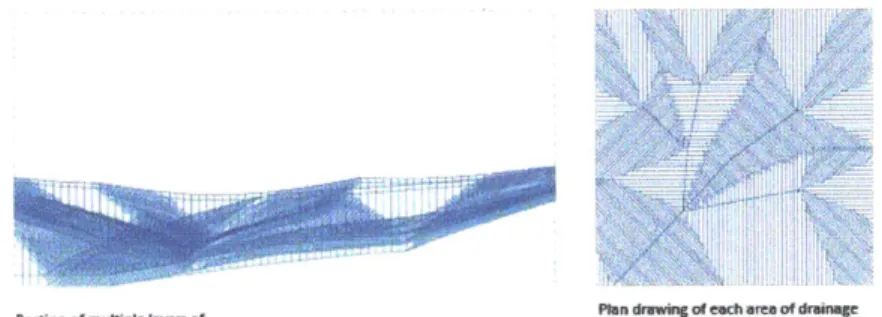
Figure 2.5. Surface Generation Algorithm 3.

Plan drawing of each area of drainage

Sectionwhich resut in the original fw pttrn

(19)

Chapter Three: Surface Data Structures

p 19

(20)

3.1 Introduction

3.1.1 Surface Definition: History

Prior to inventing a new geometrical methodology to generate complex surfaces , it is necessary to obtain a good understanding of a geometry and definition of surface from different points of views. The author of this research is interested in The definition of the surface data structure histori-cally and mathematihistori-cally to find a way to describe complex surfaces with simple graphs. In this respect, through this chapter, he will explore the idea of surface data structure in mathematics and geo-computation to build a basis for regenerating a surface using only plan drawings.

Probably Cayley, in 1859, [Cayley 1859] was the first person to describe the surface data structure. He defines different areas of a surface based on the term indicatrix or contours. He provides a grammar with his explanation and describes the properties of the most important points of a topography. (Fig. 3.1)

a. b. c.

Figure. 3.1. a. Circular Indica-trix b. Hyperbolic IndicaIndica-trix c. Parabolic INdicatrix

indicatrix is a circle in indicatrix is a hyperbola in indicatrix is a parabola

immit and summit knot in ridge and course lines

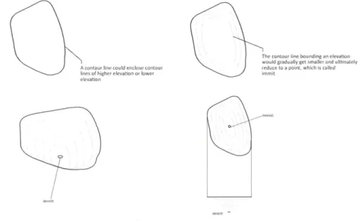
According to Cayley There are three types of indicatrix in the whole area of a continuous topography: circular, Hyperbolic and parabolic. He defines each indictrix as a closed curve which encompasses other indicatrix inside itself. By the time that we travel up in z direction, the indicatrix becomes smaller and smaller till it turns into a point called Peak or Maximum (Fig.

3.2).

Figure. 3.2. a. indicatrix or contour is a closed curve b. It encompasses other smaller indicatrices inside c. By

Trav-elling in z direction the indi- The contour we bounding an elevation

catrices become smaller and

_{beco e s allr}

_{a d}

would gradually get smaler and ultimately

A contour line could enclose contour reduce to a point, which is calied

smaller and finally become a in"of'igher"eevation or lower surnmit

peak point

20

(21)

| Computational Interpretation of Flow Pattern Drawings

Based on the same notion, if travelling in the z direction down, the indicatri-ces become smaller and smaller till become the local pit point or minimum. The indicatrix around the local minimum and maximum is circular. There is a point in topography where three indicatrices meet one indicatrix. This point is called the saddle point (Fig. 3.3).

Fig. 3.3. a. indicatrix or contour is a closed curve b. It encompasses other smaller indicatrices inside c. By Travelling in (- z) direction the indicatrices become smaller and smaller and finally be-come a minimum point

T

re

A contour line could enclose contour lines of higher elevation or lower e levation

he contour line bounding an elevation ould gradually get smaller and ultimately duce toa point, which is called nmit

The indicatrix in this point is hyperbola. If we move from a saddle point

upward we will arrive to local maximum and if we move down ward we will

arrive to local minimum. The indicatrix along the path which connects the

saddle point to maximum and minimum is parabola. (Fig. 3.4)

Atsome moinis in the terrain,

a conour ine ay meterthree

contour ines of the equal elevation

a.

At these points the cartace is Immorta

andaone deends intheiackward and the other ascends in backward

b.

Figure. 3.4. a. There is a point in topography where four indicatrices meet eacho-ther. b. the contours in this

point look like hyperbola c.

Saddle point of topography

c.

These Pohints are calied Keats At these Points the surface Is hnrizntal andnone decends inthe backward and

the other ascends in batward

p

(22)

Figure. 3.5. a. The drainage

patterns are always

perpen-dicular on contour lines b. There is only one pathe exist, if we travel from saddle point with steepest paths upward or downward which connect saddle point to maxima and minima. c. series of drainage paths on the topography. d. plan view of slope paths and contour paths

Slope Lines are perprtdtoolar to conto looes

A"idgelinould rech from n lmmit to another

immuvi ta sigletervning~o

b.

a.

ourse

Ridg"

at the knot there are two orthogonal

slope mos, which bist two OPtosite

cotoor line hyperbols, this paw of slope Ines is the Ridge and Course lnes

c.

d.

Cayley also mentions that if moving from the saddle point upward with

the steepest slope you will reach to local maxima and moving downward

will take us to the local minima. This path always perpendicular on contour

lines. If we stat from the local maxima or local minima try to go up or down

in multiple direction and in each direction we travel based on the steepest

path, we will have a family of paths which are perpendicular on contours.

These paths are called water drainage patterns. (Fig. 3.5.)

Maxwell in 1870 completed the intuitive description of surface data

struc-tures [Maxwell 18701. He divided the whole topography into hills and dales.

In describing these notions, he points out the local maxima and minima and

saddle points and the lines which connect these points to each other. Then

he explains that if defines dale or valley as area which is surrounded by

three local maximum. As a result, if we travel from one maximum to saddle

and from saddle to another maximum and again to saddle and to the third

maximum, we will establish a valley. There is a mathematical relationship

between the number of maxima and saddle points, according to Maxwell.

(Fig. 3.6, 3.7)

The number of peaks minus number of passes equals to one and number of

pits (minima) minus number of passes (saddle) equals one:

Peak - Saddle =

1

Pits - Saddle = 1 Peaks + Pits - Saddle = 2

p

22

A ridgeie wold each froom nitto aother itviraigle witerng knot Of minuT imai sumi Kont

(23)

Figure. 3.6. a, b. Local maxima and local minima and saddle points on the to-pography. c, d dale or valley. e,f. Hills

two regions of elevason and depression on thesurface define the surface in mainly three ways, Firstly, two regions of depression

would eopand until they meet up at a point, which is calld a bar

*.13~

/

Figure. 3.7. Relationship be-tween Peak, Pits and passes (Maxima, minima and Saddle

points) Peaks + pits - Passe

Peaks -T r wo n f depr n my ed o.t ofdpesc.

a.

b. Valley or Dales Regions of Depression Dale It Valley or Dales Regions of Depression Dale I c. d.

e.

f.

s = 2 2

Passes = 1 3Pils -Patses 1

P

23

7

(24)

3.1.2 Surface Definition: Mathematical Representation

After Cayley and Maxwell, Morse in 1945 [ Morse 1965], presented the mathematical definition for important points on the surface and their con-necting graph. According to Morse, the second derivative of the surface in two major direction of its curvature are responsible for establishing the critical points on the surface. If traveling from saddle point to each local ex-tremum points, we should always travel along a path on which always one of the primary curvatures of the surface is zero. (Fig. 3.8)

Figure.3.8. a. Saddle point Mathematical definition. b. Local Maximum. c. Local Minimum d. Coarse line, the line which connects saddle point to maximum points. e. Ridge lines which connects

saddle points to minima a.

b.

Saddle 621: 5.

Derivative Expression > 0 < 0

Point that Lies on a local convexity that is orthogonal to a local concavity

Max

Derivative Expression '

-Point that Lies on a local convexity in all directions (All Neighbors lower)

Derivative Expression &

Point that lies in a local concavity in all directions (all neighbors higher)

Channel Dervative Expression C. Ridge 2. Dervative Expression ~

0

~ 0

Point that lies in a local convexity that is orthogonal to a line with no concavity / convexity

Point that lies in a local concavity that is orthogonal to a line with no concavity / convexity

6 p

d.

24

g 62:

(25)

3.2. Surface Network Extraction Methods

Critical graph is the basis for lot of areas of research in GIS and geo-com-putation. Researchers in these fields use critical graph ideas to extract the most information of the complex surface of the earth and represent it with simple graph ideas. This helps them reduce the amount of space and effort they need to store the information about the geometry of the terrain. In current research, author visited the idea of surface network extraction to earn the different properties of surfaces with respect to network represen-tation of it. Consequently, chosen surface network extraction method is after (Schneider. B. and Jo wood 2004].

This method is called extraction from bilinear surface patches. In this method the whole surface geometry is subdivided into point grids. For this reason a 2 dimensional point grid is projected onto the surface. The reason for this is to have square modules of surface patches with corners sitting on the geometry of the original surface. There is a difference between the method used in this experiment and the method which is used in geo-computation field. In geo-geo-computation there is no surface exists at the begging and the process of extraction is based on digital elevation model of a terrain. (Fig. 3.9)

Figure. 3.9. a. Projecting a point grid onto the geometry of a surface to construct square surfac patches b. locations of extermum points of the surface as well as the saddle points

a.

Extraction of bllneer patches trom a given surface the size of the grid has a direc Inluenrre o n the odation of

network surface and local minimurm and

mraxirrrur poirts as wsell as pasts poirds

Local Maximum

Local Minlmum Local Minimum

Locat Maximum

b.

p

(26)

The reason for choosing the bilinear surface patches is that the properties

of extremum points of a surface can be easily discovered. In order to do so,

each surface patch is compared with its surrounding neighbors to define the

maximum, minimum or saddle points. For maximum and minimum points

the property of the surface patches is quite easy: if the central vertex has a

height bigger than its surrounding neighbors, then the point is maximum. If

the height is smaller than that of surrounding neighbors, then the point is

minimum.

For saddle point there are two possibilities: first, there is a possibility that

the saddle point happens on the grid. This means that the neighbors are

higher and lower alternatively. Second, the saddle point might happen in

the middle of the surface patch. This means that the corners of the surface

patch is alternatively higher and lower. (Fig. 3.10)

a.

Tm PossiAA mfiguat m wAA bonw surapatc hAA w

! t. P at

Figure. 3.10. a. Surface patch and central vertex and its surrounding. b. Saddle point on the surface. c. Saddle point on the grid. d. 4nimum point e. Maximum Pgipt.

b.

d. mqgaA a.-Aghe,

d.

c.

e.

Bdinmr Surtwe P ch Ev"cbon fm Surf Net- k

(27)

Pass Pat Ithe oldie of sufface patches

ciij

Pass POWt I on

the gidi of patch surfaces

Figure. 3.11. Locating the saddle points on the topography and finding the

principal directions to go up or down

The process of the surface network extraction starts right after the process

of locating the saddle points. Since the graph is achievable connecting the

saddle points to maximum and minimum (Fig. 3.11). for this reason we

need to find the steepest path from the saddle points to take us to the

maximum and minimum points of the surface. There are two conditions

based on the location of the saddle point. First, is the saddle point on the

surface patch. In this condition, the starting points for up and down

move-ment is chosen based on their heights. The second condition is when the

saddle point is on the grid. In this case, the starting point will be based on

the surrounding neighbors.

p 27

(28)

---Designing Performative Surfaces

Figure. 3.12. Different

reso-lution of path finding. a. 45

Degree Resolution, top path -

-downward, bottom, path

upward. b. 30 degree

resolu-tion, top path downward,

bottom, path upward. c. 7.5

- Sl-p t - S - 1

degree resolution, top, path downward, bottom, path

upward / s P PR P S S S Xw w Fl Pat-orr

a.

b.

c.

There are also different resolutions to find the steepest paths along the

surface. The 45 degree resolution only finds the steepest paths in 8 primary

directions, while 30 degrees and 7.5 degree and so on provides finer

resolu-tion of paths for the surface network graph (Fig. 3.12)

Continuing the path finder algorithm results in clear surface network

pat-terns. Having this graph helps us understand the behavior of the surface

with respect to the shape of the graph and the overall geometry of the

topography (Fig. 3.13). This graph would be the basis for this research to

reconstruct complex geometry using plan drawings.

(29)

Figure. 3.13. a. axonometric view of the surface with its surface netwrok graph. b. plan view of the surface with surface netwrok graph.

0 Pit Pit Peak Pass Pit P Pit b. p 29 Pit

(30)

3.3. Regenerating Surface Using Surface Network Graphs

So far we learned how to extract the surface network graph from the geometry of a given surface. Form this step it is important to generalize the topologies of surface network graphs and control them to reconstruct the surface geometry. In (Fig. 3.14) the general topology of surface networks

are represented. [ Surface network graph]. in the step of the process the

most simple network is chosen to extract the contours for the reverse pro-cess of surface generation.

a \ /XIh 2 Ma, Sd&. :M., --- --- !7. dk, towioqcal pattern of r1ao nelwrol, ,otcal potnt coolkfunatton

M..

%

4 ...

"l-Figure. 3.14. a. axonometric and elevation view of general surface netwrok diagram. b.

Plan view of different types olpsurface network after

I F3ia 2002].

(31)

Max

Saddle

Z6

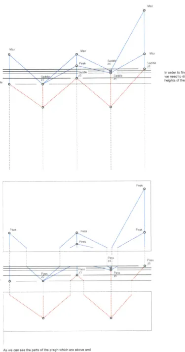
-a In order to find the contours of the pragh

Saddez3_Saddle we need to divide the graph based on the

heights orf the peos poinds

Figure.3.15. Subdivision of the graph into three main parts: upper, middle and lower parts.

Peak Peak

bPmg p ___ ___ ___ __Z4__ Pass.

contain the local maxirna and local emma of the graph aed consequently the contours are closed curves around those

Based on this notion the author developed an algorithm to extract the

contours from the network and reconstruct the surface. In order to extract

the contours, we need to divide the whole graph into mainly three parts Fig. 3.15) upper part, which includes all the peak points. Contour lines in this part of the graph is closed curves. This can be proven using the [Cayley

18591 grammar of a surface. According to him indicatrix around local

maximum or minimum points of a surface is a closed curve and circular.

The Lower part can be derived respectively. The most import point in this

subdivision is the location of the middle part or the lower bound of upper

part and the upper bound of lower part. p

Fig 3.5) ppe pat, hic inluds al te pak oins. ontur in 31i Max

(32)

For the upper part of the lower part, if we search among the saddle points and find the one which has the lowest height among the others, then that can be used as the basis for the boundary between the lower part and the middle part. For the lower bound of the upper part, if we find a saddle point which has the highest height among the others, that would be the upper bound for the middle part (Fig. 3.16)

Intersection Plane * 4,Mmn Min

a.

Intersection Plane Axonometric drawing of the network Max Max Max

Figure. 3.16. a. The lower part of the graph and lower bound of the middle part b. upper part of the graph with the upper bound of the middle part.

p/

32 _..._.

(33)

saddle Saddl 3 Saddle Z1 Saddle 4 Saddle z5 Saddle )D Intersection Plane Intersection Plane

Figure. 3.17. a. Middle part of the graph

b. Completing the contours by adding all parts together

Intersection Plane ---

---a.

Wa ag A. / / / 7

---

--

-b.

By Extracting the contours from each part we will be able to have

continu-ous closed curves to reconstruction of the surface. The importance of this

algorithm relies on the fact that since these contours are extracted from a

particular curves in the graph, there is no order in terms of connecting the

curves and making a continuous closed contour curve which travels along

the whole surface (Fig. 3.17)

p

(34)

Designing Performative Surfaces Mu x ss, V.ame /~> ~-j~o 2~

Figure. 3.18. Topologically Similar networks

4

There isa possiblty of translating

any geometrical pattern and grid nto landscape orgazation usin

surface network graph

Developing the contour extraction algorithm allows us to extract the

contours from any given network graph and consequently reconstruct the

surface using the contours. This means any given graph that is topologically

related to the idea of surface network can be used to generate topography.

(Fig. 3.18). Shows some design possibilities of a simple network and

inter-changeability of them. This is an important point for designs, since one

graph can provide multiple design options.

Lets take a look at a simple design possibility of network graph. In This

ex-ample, designer starts with a simple module of surface network graph and

aggregates them to create a topography. Simply this aggregation can be

used for contour extraction algorithm and eventually the surface

topogra-phy will be constructed based on that. (Figure. 3.19)

p 34

(35)

Saddle Max

Max

Aggregation of simple Saddle netwrok graph and its subsequent topography Saddle M a. /Max / Saddle a Max b. Figure. 3.19. a. Simple-module of Surface network Graph. b. Aggregation of the module c. Contour extraction result d. Final topography

c.

Contour E xtractin process

d .

p

(36)

The key point in generating the surface with this technique is the variability

of the result based on the contour manipulation. Secondary design

algo-rithms can be used in this step to change the simple definition of contour in

different types of curves. (Figure. 3.20)

In current example the regular sharp connection of contours are changed

step by step using chamfering algorithm. This algorithm searches for

inter-section between the contours and chamfers them based on a fraction of the

length of each intersection lines. The result is a topography with different

resolution on courses and ridges.

a.

Contour Extraction process

S41P 2 Stop

b. C. d.

Figure. 3.20. a. Extracted con-tours from the network graph with sharp angle connections b. chamfer algorithm to change the corners step 1, c. chamfered AIgorithm Step 2, d. Chamfered aS6rithm Step 3.

(37)

3.4. Summary

In this chapter the general idea of surface construction using graphs was in-troduced. The material for this chapter was gathered from different science fields such as computation a geometry, geo-computation and geographical

information science. Consequently, the history of surface data structure was visited. The term critical graph and it use in geo-computation was the main area of containers of this chapter. Further on the process of topography generation from critical graph was explained and some example of the use of such techniques in terms of design was provided.

p 37

(38)

Chapter Four: Generating Performative Surfaces

P

(39)

4.1. introduction

In this chapter the author will introduce three main algorithms based on the foundation of the surface netwrok graphs. The surface netwrok graphs are not directly used in the generation of these graphs but lessons Ireaned from the performance of the surface was nessasry for the results of this

chapter. The Algorithms provided in this chapter are chronologically related meaning that they complement each other and the earlier algorithms are the ancestors of the last algorithm.

4.2. Performative Aggregation of Critical Graph

In this section, lets take a look at the properties of a single critical graph. mentioned in chapter 3, each complete graph consists of three types of points: Maximum, Minimum, and saddle points. and two types of lines: Ridge lines are the ones which connect saddle points to minimum points. Coarse lines, on the contrary, connect saddle points to maximum points. change in the height properties of each of the graph's points will change the whole properties of the graph as we can no longer call that a complete network (Fig. 4.1) Max Sadl Saddle 0: saddle -Saqdle or , ma a. Ma-b. Max

Figure. 4.1. Change in height of each point of the graph changes the properties of the graph. a. complete graph b. Graph with incomplete ridge coarse lines c. graph with incomplete ridge and coarse lines d. graph with new ridge lines. Max "pde 9 Sad* Max Md.

d.

c. p 39 Sadde d

(40)

aggregation

of

the

surface netwrok graph is a method of reconstruction

of surface. observation from the characteristics of the netwrok shows the

possiblity of reconstruction using only ridge lines (Fig. 4.2). if we reverse the

order of surface reconstruction,The key point is the change in height of the

points. if we start from the zero elevation height, in order to construct

sur-face, we need to create ridge lines. This obsrvation is the basis for deriving

surface reconstruction algorithms which are provided in this research.

Figure. 4.2. a. Side by Side Aggregation of the Surface network units. b.

descend-ing aggregation of the surface

-networks.

a.

b.

4.3. Surface Generative algorithm version 1

This algorithm is based on point grid transformation in three diemensional

space. The assumptions in this approach is that the surface will be

con-structed on a starting point grid field. Surface reconstruction is acheived

through activating each cell on th point grid to create ridge line. the

Algo-rithm is operated in each step and continues till the last cell of the point

grid is activated. In order to create the first ridge line, all the points of the

point grid are transported to higher elevation except the starting point (Fig.

4.3). in the next step all the transported points, except the ones that are

connected to the both sides of the ridge, are transported again to higher

elevation. this technique genrates connected ridge lines as well as coarse

lines on the surface. the process continues, untill all the surface truns into a

connected networks of ridges and coarse lines (Fig. 4.4)

Figure. 4.3. Step by Step Trans-formatin Algorithm

Grid Transformation Algorithm 1 Step 2 Step 3 Step n

Step 1 The gray area Inactive area all the surface

is the inactive area becomes smaller is active

Step 2 Step 3 Step n

Grid Transformation Algorithm 1 The gray area Inactive area all the surface

p Step 1 is the inactive area becomes smaller is active

(41)

topography result of the process

Step n

Step 4

Step 3

Figure. 4.4. Surface transforma-tion Algorithm

Step 2

Step I

P 41

(42)

Designing Performative Surfaces ' >\ Step n Propagation of drainage pattern step n-i /*> Step 4 X-> 7

'

Step 3 Step 2 Step 1

a.

b. _{Step n} _{step n-1} _{Step 4} _{Step 3} Step 2 Step 1

Inactive nodes on the point grid

947', 1',

C.

The process of transformation has different steps. In Fig. 4.5, The

propaga-tion of ridge lines are shown as well as the activation steps for each cell till the last cell. The most important factor that need to be mentioned is the whole process is starts with drawing a line on the flat point grid. This will provide a control for the designer to transform the surface based on the original flow pattern that s/he input to the surface. Figure 4.6 Shows the

physical model of the process.

4.4. Surface Generative algorithm version 2

Figure. 4.5. Different results of algorithm through the comple-tion process. a. Propagacomple-tion pro-ceps b. Cell activation process c.

r

gfce

transformation process

This algorithm is in connuatio of the previous algorithm with some

modifi-cation. The previous algorihm results in more dynamic surface generation

which might not be ideal for architectural porposes. in this respect, the

Author modified the process of algorithm to acheive smoother surface.

Accord igly, in this algorithm the transfom ration of the grid into higher

elevation is modified throuygh just moving the points that are not shares

with the activated cell.

(43)

7-Computational Interpretation of Flow Pattern Drawings

Figure. 4.6. Physical Model of the

transfor-mation process p

(44)

This process helps creating smoother and cleaner ridges and entually

cleaner topography. in this algorithm, similar to previous one, the designer

inputs the flow pattern drawing and surface transfromation is based on

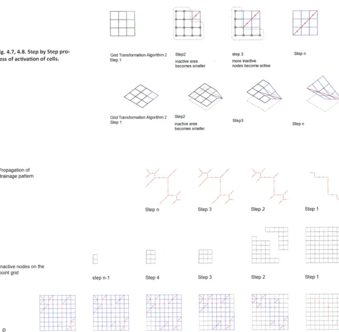
ridge generation process (Fig. 4.7, 4.8, 4.9)

W-iJ

Fig. 4.7, 4.8. Step by Step pro-cess of activation of cells.

Propagation of drainage pattern

Inactive nodes on the point grid

44

Grid Transformation Algorithm 2 Step 1

Grid Transformation Algorithm 2

Step 1 Step n step n-1 Step 4 Step2 inactive area becomes smaller Step2 inactive area becomes smaller / /

3.

/ / Step 3 Step 3 step 3 more inactive

nodes become active

Step3 Step 2 * I Step 2 ---- -7

-1.

dL

Step n Step n St

]1

Step 1 Step 1 ---

(45)

---cr.

3!

Oa0 3 e a

~.0

_CD0 -0 U, cn <D'a (D 'a CD. cl) . ... . . ... ..

(46)

a.

Figure. 4.10. a. Algorithm 2 b. Algorithm 1

Comparing the topography results from the two algorithms reveals their inherent differences (Fig. 4.10) obviously, the second algorithm generates smoother and cleaner surface, but this shouldn't overshadow the inter-esting features of the first algorithm. The first algorithm, regardless of its complex geometry can transfer flow in multiple directions and create more dynamic flow of water. The second algorithm, on the other hand, provides with a faster and shorter paths for the flow. The most important disadvan-tage of both is the low resolution of the input drawing and also the result. Moreover, the drawing cannot handle angles more or less than 90 degrees and this is a limitation for design and generating performative surfaces.

p 46

(47)

4.5. Surface Generative algorithm version 3

This the third and last algorithm provide in the research which is developed

to overcome the problems and disadvatanges of the previous algorithms.

flow of water always follows the shortest paths on the surface or

topog-raphy. this algorithm is founded based on the idea of shortest distanc of

point grids to the input flow drawings. similar to previous algorithms the

surface is a result of transfomrtaion of point grid in three dimensional

space.

(Fig. 4.11). in this the shortest distance of each point with respect

to the flow patterns is calcualated (Fig. 4.12). unitizing the shortest

direc-tion for each point on the grid will result in a discontineous field of lines

and points. in order to create a continuoue filed of lines and points Author

developed a rationalization algorithm for the flow direction. this simple

algorithm creates a connected netwrok of lines and points which also

reprsent the dirction of the flow at each poin of the point grid (Fig. 4.13)

.

4.5.1. Rationalized drainage direction of a surface

osmest distance to line segment

simple dista e function foreach

point on the grid which finds the

b. '""'"""o""* e**

Figure. 4.11. a. Point grid b. input Flow pattern on the point grid

Figure. 4.12. a. Point grid b. input Flow pattern on the point grid

In order to explain the process of this rationaliaion, lets have a closer

look at the unitrized field of ponts and flow directions [ Figure. 44]. for

each point there exist eight souraounding neighbors. the direction which

connects each point to its sourounding points is considered a primary

direction. this allows us to create a connected netwrok of points and lines.

in order to rationalize the direction of the flow, the angle of the unitized

vector is complared to the primary direction for each point. the mimum of

these angles is chosen and the corrsponding primary direction is drawn to

create a connected netwrok of flow. [Fig. 4.13).

-M

a.

Closest distance to line segment Simple distance function for each point on the grid which finds the corresponding point on the line segment

b.

Unitized closest directions to the line segements

a. Goit xid

GridSize :50 xl

p 47

(48)

Designing Performative Surfaces Rationalized Direction j -1, j+1 Shortest Distance Direction

[Z77

j, j+1

For each Point there are eight surrounding points that can be compared for the ratioalization algorithm

Figure. 4.13. each cell is com-pared to eight primary directions of the flow to rationalize the unitized direction vector

Rationalizing the direction The algorithm is looking for the

minimum distance of the test direction

with eight primary directions and rationalize the direction with the primary direction.

The algorithm of minimum angle also counts for compliment angle between two vectors so it generally solves for 16 possiblities

Thistechnique is used to test the flow representation on the surface. fr this

reason a complex surface was choosen to reflect the direction of the flow.

first a 2 dimensional point grid projected on the surface. from each

project-ed points the steepest path was calculatproject-ed basproject-ed on the resolution

men-tioned in chapter 3 (Fig. 4.14, 4.15, 4.16). diffrent steps of flow will result in

differnt paths on the surface.

if we use the same techniue of rationalzation for the flow direction, we can

reconstruct the gometry of the surface with a connected network which

represents the direction of the flow on the surface as well. in order to cover

th whole area of the surface, this technique needs to be applided in two

opposite directions: steepest path up, and steepest path down. this will

cover the whole area of the surface

[

Figure. 46]

p

48 j+1, j+1 j+1,j-j+1 , j-1 0 a

(49)

\ . .. .. .. -\ \ \ \ .... I.I.I. 11~ U-1--(6 a.S H $2 J .. . . . -6 -If C . * * 0 . vi C) U 3 w C c c o TC 0 0 0 U C(CL000 0 0

D

"~co'o

(50)

Designing Performative Surfaces Slope finer 46 degrees resolution 20 steps of slopes Inverse Slope Super imosition of both layers to cover the areas that has no connection to the rest of the netwrok

Slope

C.

Figure. 4.15. Slope Finder algorithm a. upward direction

b. Downward direction c. super-im osition of both d. surface , wrok grah layered on top of

h~ow pattern

a.

inverse 46 degrees Slope resoltionfiner 20 steps of slopes

7.

(51)

S[ctural model made based m

Superimpo5itionofWatefshed5Bfd

4 11 11P

erse water Stieds

Figure. 4.16.spatializing the flow

patterns. note that the geometry is not very clean since there is no rationalization applied yet.

(52)

Figure. 4.17. Flow path finding on another type of surface with different resolutions.

Figure. 4.18. a. Flow pattern finding algorithm 45 degree an-gle resolution 50 steps of slope finding b. 45 degree of resolution first step of slope finding c.

Con-The same technique was also used for different types of surface to see the

possible differences. This technique also helps recognizing the surface

net-work graph of the surface (Fig. 4.17). by using this technique it is quite easy

to cover the whole area of the surface with straight elements which meet

each other at 45 degree angle in plan projections (Fig. 4.18, 4.19, 4.20]

.

Firs stepof rationallzation of the

b.

Final Step of Rationalzation based on 45 degree eolution

c. p

52

Original Water flow Algorithm result (fo

agrId 60X60on a given topography

a. 73 dn- I.Wlft 20'"" tr 20 s". me., 70 MW h'- SIM MMr 7 dw. -A*. 2D V

(53)

PI.Vl-Computational interpretation of Flow Pattern Drawings

Figure. 4.19. Physical Model of

the rationalized surface based on p

(54)

Figure. 4.20. Physical Model of the rational-iz@d surface based on flow direction

(55)

77

Rationalized directions of the closest point

Figure. 4.21. a. Rationalized o

connected network b. Unitized

shortest distance direction c.

Shortest distance drawn from Unized closest directions to Closest distance to line segment

each point on the grid to the the line segements Simple distance function for each point on the grid which finds the

corresponding segment of the corresponding point on the line segment

4.5.2. Algorithm description

If we use the smae tecnique for the two dimensional point grid, we can

have a connected netwrok of lines which author tends to call the influence area of each segement of the flow drawings (Fig. 4.21). this simplifies the surface generation algorithm since the point grid has been divided into descrete segments which are under the influence of each segement of the line. One of the key points in constructing connected drainage network is that the process of rationalized direction must be applied twice in two complete oposite direction from eachother tocover the whole area of the point grids (Fig. 4.22)

Now that we are dealing with each segment seperately, we can measure the shortest distance from each point and transalte that into third

dimen-sion adding to its height component (Fig. 4.23, 4.24, 4.25). changing the z p

(56)

Rationalization Algorithm Reversed Rationalization Algorithm

/

Paints which are cover

Rationalization Algorithm Reversed Rationalization Algorithm

-U

Rationalization Algorithm Reversed Rationalizatio Algorithm

Figure. 4.22. a. Rationalized connected network b. Unitized shortest distance direction c. Shortest distance drawn from each point on the grid to the cor-responding segment of the line.

Areas of over lapping between rational and reverse rational distance algorithm

b.

superimposed both rational and its reversed algorithm on the point grid to cover all connections between grids

C.

p 56

(57)

// PLk i PL k PLkO Poytine segmentation

b.

The area of influence of each segment of lines LP Point ij PL ki 0 PL k i Point i

The algorithm of tranforming the two dimensional points of influence to three dimensional points

C.

Area of influence of fine segment PL ki

Projected point grids in the area of influence

d.

PL k

Figure. 4.23. a. area of influnce of each segment of the line b. line segments of an input polyline c. plan distace from the point to corresponding line segment d. linear translation of distance to height e. three

a.

A

(58)

iteration 01 slope = % 0.0 iteration 01 slope = % 0.1 iteration 01 slope = % 0.3 iteration 01 slope = % 0.6 P 58 ----

(59)

---Computational Interpretation of Flow Pattern Drawings

Projected or two-dimensional netwrok

3-dimensional geometry resulted from the planar curve

Elevation Drawing of the generated geometry

Figure. 4.24, 4.25. Different fraction of z creates different surface slope fom completely flat to one to one relationship between the plan distance and height

Plan view of both three-dimensional and projected netwroks

p 59

(60)

4.5.3. Global Drainage Designing Performative Surfaces

So far we achieved surface generation algorithm using shortest distance

in plan projection. This allows designers to start with planar curves and

construct surfaces which drain into the planar curves (Fig. 4.26). What if the

global drainage of the surface is intended. In other word, how to construct

the surface that can drain along a curve. For this reason we need to first

reconstruct the curve in three dimension as if a drop of water starts at the

highest point of the curve, it follows the slope of the curve without

chang-ing its oath along the curve till it arrives to the lowest height of the curve.

There are three major types of curve, which can be used in this algorithm:

poly lines, control point curves, and branching control point curves [ Figure.

58]. The process of constructing spatial curve is quite simple. Each time the

control points of the curves are calculated and based on the input slope

pa-rameter and length of the curve, the height of each control point is

adjust-ed. The result is a spatial curve which cannot sit on a single plane in three

dimension space. For branching geometry the method is still the same with

a difference that in branching poly line, each time, the designer must draw

the poly line from the root.

h t

t Ili tIr

Et COjri i

t P k

a.

t (n) -end domain of the line

t (0) = Start domain of the line

h = desired starting height (designer input)

h (i) =h *t (i) *(t (n))^(-1) tt Z.iv

b.

P7-n t tt c . Pok PCw P~n PE k

Figure. 4.26. a. Spatial poly line generation b. Spatial curve c. Spatial branching poly lines and cggrol poly lines

Designing performative surfaces : computational interpretation of flow pattern drawings