HAL Id: tel-01699030
https://tel.archives-ouvertes.fr/tel-01699030v2
Submitted on 1 Mar 2018HAL is a multi-disciplinary open access archive for the deposit and dissemination of sci-entific research documents, whether they are pub-lished or not. The documents may come from teaching and research institutions in France or abroad, or from public or private research centers.
L’archive ouverte pluridisciplinaire HAL, est destinée au dépôt et à la diffusion de documents scientifiques de niveau recherche, publiés ou non, émanant des établissements d’enseignement et de recherche français ou étrangers, des laboratoires publics ou privés.
Benjamin Khiar
To cite this version:
Benjamin Khiar. Laboratory astrophysics with magnetized laser-produced plasmas. Astrophysics [astro-ph]. Université Pierre et Marie Curie - Paris VI, 2017. English. �NNT : 2017PA066310�. �tel-01699030v2�
pour obtenir le grade de docteur délivré par
Université Pierre et Marie Curie
École doctorale d’Astronomie et Astrophysique d’Ile-de-France
présentée et soutenue publiquement par
Benjamin K
HIAR
le 26 septembre 2017
Laboratory astrophysics with magnetized laser-produced
plasmas
Directeur de thèse : Andrea CIARDI
Jury
M. Philippe Savoini, Professeur Président
M. Petros Tzeferacos, Research scientist Rapporteur M. Emmanuel d’Humières, Maître de conférences Rapporteur Mme. Catherine Dougados, Directrice de recherche Examinateur
M. Émeric Falize, Ingénieur CEA Examinateur
Contents iii
1 Introduction 1
1.1 The context: High Energy Density Laboratory Astrophysics (HEDLA) . . . . 2
1.2 The thesis environment . . . 3
1.3 What you will see in this manuscript . . . 5
1.4 Bibliography . . . 6
2 MagnetoHydroDynamic 9 2.1 Introduction . . . 10
2.2 Fluid equations from the kinetic theory . . . 12
2.2.1 Zero-order moment: the mass conservation equation . . . 12
2.2.2 First-order moment: the momentum conservation equation . . . 13
2.2.3 Second-order moment: the energy conservation equation. . . 16
2.3 MagnetoHydroDynamic (MHD) reduction . . . 16
2.3.1 Summary of the multi-species fluid equations . . . 16
2.3.2 Expression of the collisional heating term . . . 18
2.3.3 The conservation energy for multi-species fluid equations . . . 19
2.3.4 The bi-temperature MHD model. . . 20
2.3.5 MHD mass conservation equation. . . 21
2.3.6 MHD momentum conservation equation . . . 21
2.3.7 MHD internal energy conservation equation. . . 24
2.3.8 The generalized Ohm’s law . . . 25
2.3.9 The displacement current in the Maxwell-Ampere equation . . . 30
2.3.10 Relative importance of the various electric field terms in the general-ized Ohm’s law . . . 31
2.3.11 The induction equation . . . 35
2.3.12 The quasi-neutrality assumption . . . 36
2.3.13 Conservation of the total energy in the MHD model . . . 36
2.4 The GORGON 3D resistive, bi-temperature MHD code . . . 39
2.4.1 Introduction . . . 39
2.4.2 Implemented equations . . . 40
2.4.3 Localization of the physical quantities in the GORGON grid . . . 40
2.5 Implementation of a laser module in the GORGON code . . . 41
2.5.1 Introduction . . . 41
2.5.2 Electromagnetic Wave propagation equation in a (unmagnetized) plasma . . . 42
2.5.3 Effect of electron-ion collisions on the propagation of light waves in homogeneous plasmas . . . 45
2.5.5 Implementing the laser deposition module in the three-dimensional,
resistive MHD code GORGON . . . 47
2.5.6 Validation test for the laser module . . . 50
2.6 Implementation of the Biermann battery effect in the GORGON code . . . . 52
2.6.1 General description . . . 52
2.6.2 Details of the numerical implementation . . . 53
2.6.3 Simulation tests . . . 54
2.7 Bibliography . . . 57
3 The physics of laser-solid target interaction 61 3.1 Introduction . . . 62
3.2 The ablation process . . . 63
3.2.1 Material removal by laser energy . . . 63
3.2.2 The mediating effect of the ablated material . . . 64
3.2.3 General picture of a solid target illuminated by a laser pulse . . . 65
3.2.4 Temperatures reached in laser-produced plasmas . . . 70
3.2.5 Scaling laws for laser-produced plasmas parameters . . . 71
3.3 Dynamics of laser-produced expanding plasmas . . . 71
3.3.1 Introduction . . . 71
3.3.2 Adiabatic self-similar 1D plasma expansion . . . 72
3.3.3 Isothermal self-similar 1D plasma expansion . . . 80
3.3.4 A new potential 1D description of laser-produced plasmas expanding at supersonic/hypersonic speeds . . . 81
3.4 Bibliography . . . 88
4 Physics of supersonic jets and shocks 93 4.1 Introduction . . . 94
4.2 A little bit of history about supersonic jets and shocks . . . 94
4.3 The propagation of unmagnetized supersonic jets in an external background . . . 97
4.4 Stability of unmagnetized supersonic jets . . . 100
4.5 GORGON simulations of supersonic jets . . . 103
4.5.1 General description of a pressure-matched supersonic jet . . . 103
4.5.2 Effects of the Mach number on jet propagation . . . 109
4.5.3 Influence of an axial magnetic field on the dynamic of a supersonic jet . . . 111
4.5.4 Supersonic jets propagating in a magnetized vacuum . . . 115
4.6 Bibliography . . . 116
5 Generation of astrophysically-relevant jets in the laboratory 119 5.1 Introduction . . . 120
5.2 Experimental production of magnetically collimated jets . . . 120
5.3 Initial numerical setup and laser parameters . . . 123
5.4 General plasma dynamics . . . 124
5.4.1 Velocity profiles . . . 126
5.4.2 Density profiles . . . 127
5.5 Cavity formation and evolution . . . 129
5.6 Jet structure and dynamics . . . 133
5.7 Jet 3D instabilities . . . 134
5.9 Influence of a gas background and mitigation of the Rayleigh-Taylor
insta-bility . . . 142
5.10 Frequency resolved radiations imaging . . . 144
5.11 Influence of the spatial resolution on the jet 3D structure . . . 145
5.12 Bibliography . . . 147
6 Toward controlling the temporal properties of laser-produced plasma jets 151 6.1 Introduction . . . 152
6.2 Experimental and numerical setup. . . 152
6.3 Results . . . 153
6.4 Bibliography . . . 158
7 Generation of unstable supersonic plasma pancakes in strong transverse mag-netic fields 161 7.1 Introduction . . . 162
7.2 Initial setup and lasers parameters . . . 162
7.3 General 3D dynamic . . . 163
7.4 Three-dimensional stability of the produced plasma pancake . . . 165
7.4.1 Rayleigh-Taylor instability in the MHD regime. . . 168
7.5 The effects of the plasma beta on the instability . . . 169
7.6 Experimental results . . . 171
7.7 Bibliography . . . 173
8 Accretion physics 177 8.1 Current picture of magnetospheric accretion onto young stars (T Tauri stars) 178 8.2 The accretion shock . . . 182
8.3 State of the art of numerical simulations of accretion shocks. . . 186
8.4 Bibliography . . . 191
9 Magnetized accretion in the laboratory 195 9.1 Introduction . . . 196
9.2 Experimental results . . . 196
9.3 Numerical setup. . . 199
9.4 Generation and characterization of the accretion column . . . 201
9.5 Accretion shock 3D structure . . . 203
9.6 Temperatures and emission in the laboratory accretion process . . . 206
9.7 On the importance of the obstacle ablation. . . 210
9.8 Influence of the orientation . . . 212
9.9 Bibliography . . . 214
10 Conclusion and future prospects 219
A Waves and instabilities I
A.1 General formulation from the ideal MHD equations . . . II A.2 The case of motionless homogeneous unmagnetized compressible plasma:
sound waves . . . V A.3 The case of motionless homogeneous magnetized compressible plasma: Alfven,
slow and fast magnetoacoustic waves . . . V A.4 The case of discontinuously stratified plasma without magnetic field: the
A.5 The case of a discontinuisly sheared velocity unmagnetized compressible plasma: the Kelvin-Helmoltz instability . . . XIV A.6 The case of a single magnetic stable interface . . . XVII A.7 The case of a magnetic slab . . . XX
List of Figures XXVII
Introduction
Sommaire
1.1 The context: High Energy Density Laboratory Astrophysics (HEDLA) . . 2 1.2 The thesis environment . . . . 3 1.3 What you will see in this manuscript. . . . 5 1.4 Bibliography . . . . 6
1.1 The context: High Energy Density Laboratory Astrophysics
(HEDLA)
This thesis represents one contribution to the growing field of "laboratory astrophysics" and more particularly to the area of high energy density laboratory astrophysics. First, the origin of the term laboratory astrophysics comes from the possibility to investigate astro-physical processes using human-made tools "on terra firma". This, of course, encom-passes a very large panel of different disciplines ranging from atomic/molecular physics [1;2] and condensed matter [3] to nuclear [4] and particle physics [5] For example, the fundamental question of the origins of life has been addressed in the laboratory in order to assess the possibility of a life being "seeded" by organic chemicals and water brought by cometary impacts [6]. Indeed, experiments have simulated the composition of comets and interstellar ice grains and shown that upon sufficient radiation heating and vapor-ization of these materials, it is possible to produce the building blocks of life [7]. Plasma physics is another major area relevant for astrophysical studies. Indeed, it is now well established that the vast majority of the visible matter in the universe (so excluding the hypothetical dark matter) is in the state called "plasma". Often qualified as the fourth state of matter, it is observed when the energy present in a given system is sufficiently high to ionize the atoms. This state has been "officially" first reported as "radiant mat-ter" in 1879 by Sir William Crookes and since then, the field has undergone an impres-sive number of discoveries and breakthroughs. These works have been driven notably by the "quest" aiming to mastering nuclear fusion reactions, in a controlled way, in order to produce energy. In parallel, plasma physics has been very early recognized as the good framework to study a very large number of astrophysical processes. However, it is only until recently that the human technology has reached a point where it is possible to pro-duce, in the laboratory, matters in states or regimes relevant to astrophysical phenomena occurring at high energy densities. This field is often called "High Energy Density Lab-oratory Astrophysics" (HEDLA). The lasers have a special place in this field since their invention in the 1960’s. They are indeed an amazing tool to focus (electromagnetic) en-ergy on small spatial scales and short periods allowing the generation of hot and dense materials. The foundations of HEDLA lies in the famous and relatively intuitive "nerdy" proverb: "same equations → same solutions". The mathematical translation of this sen-tence is called the "scaling" and consists simply to say that if two systems, for example one in the vacuum chamber of a Parisian laboratory and the other localized around the shock wave propagating in the interstellar medium as the result of the death of a star, obey the exact same set of equations, then their evolution will be strictly equivalent under the condition that the initial and boundary conditions are the same. Of course, the passage from one scale to another is done using certain scaling parameters and one should not be surprised to see somewhere some sentences such that "1 nanosecond of evolution of this system represents one year of this system" or "1 millimeter of this system repre-sents one solar radius of this one". This, of course, has to be understood as being a pure mathematical assertion but which can be useful from a physical point of view. One of the first topic being studied in the laboratory using lasers has been the propagation of bow shocks (in magnetopsheres, interstellar mediums, supernovae...) in the early 1990s. In this case the scaling was hydrodynamical and possible because the physical regimes (quantified by dimensionless parameters such the Reynolds number, Peclet number...) were similar. In mathematical language it is equivalent to say that both systems obey to the Euler equations (Navier-Stokes equations without viscosity and thermal conduction). Later, near the beginning of the new century, Ryutov introduced the same reasoning but
in the case where a magnetic field is present. In this case, he demonstrated the possibility to perform a strict mathematical scaling in the framework of the "ideal magnetohydro-dynamic" (MHD), even in the presence of shocks. The MHD is the model describing the behavior of neutral fluids within which electrical currents can flow (because the fluid is ionized) and thus couple to the magnetic fields. Ideal MHD is somehow, for MHD, the equivalent of the Euler equations for the Naviers-Stockes equations. The idea behind the restriction of the scaling to these "simplified" set of equations lies in the fact that dissipa-tive processes tend to break the scaling. It should however be noted that more recently a consequent work has been done to include in the scaling the possibility for the systems to be non adiabatic through the loss of energy by radiations [8]. The work published by Ryutov [9], beginning to be called the "Ryotov scaling", has been the starting point of a whole new generation of magnetized experiments aiming to study the behavior of flow when the fields are sufficiently strong to influence the plasma dynamics. One of the most studied topic in this area concerns the study of magnetized flows observed around young stars at times during which they are still accreting material from the environing medium, notably their accretion disk. Indeed, it has been discovered in the 1980s that these stars (called "T Tauri Stars" or TTS) often exhibit large outflows which can be, in some cases, highly collimated [10]. It was rapidly supposed that magnetic fields observed on these systems could be involved in the formation of these jets/winds [? ] and now it is consid-ered to be true with a high degree of certainty. Very early in the 2000’s, the plasma physics group of Imperial College pioneered the production of magnetized laboratory jets using the high pulsed power facility MAGPIE [12;13]. They used a setup producing a toroidal magnetic field pushing and collimating hypersonic radiative jets. This configuration was astrophysically-relevant in the sense that it was similar to the topology of the "magnetic tower" model of astrophysical jets [14]. In these experiments the plasma is generated by the sublimation of solid wires through mega-ampere currents delivered by capacitors in very short times (∼ µs). The magnetic field generated by these currents exerts a pres-sure such that the flow is accelerated and highly collimated. Roughly at the same time, Bellan and his team developed a platform at Caltech to study MHD jet launching using a planar magnetized coaxial plasma gun [15;16]. Their work showed strong instabilities (especially "kinks") of the jets in this configuration. In these previous works, the magnetic field was always self-produced by the currents flowing inside the plasma. In 2013, the col-laboration within which this thesis was realized demonstrated for the first time the pro-duction of astrophysically-relevant magnetized jets using external magnetic fields as well as lasers [17;18]. The difficulty to experimentally produce homogeneous and stationary (on the hydrodynamic scale) strong magnetic fields (> 10T) had for a long time prevented the use of laser-produced plasmas at high intensities (necessary to obtain the "good" as-trophysical regimes) to produce magnetized jets. The work demonstrated the possibility to collimate a diverging plasma flow into a highly collimated stable jets using a poloidal field. As we are going to see in the next sections, these laser-produced jets are somehow the "row material" of the work performed in this thesis where novels configurations using the same setup as in 2013 ([19]) are presented both numerically and experimentally.
1.2 The thesis environment
The work presented in this manuscript has been carried out during my three PhD years within the team "Plasmas stellaires et astrophysique de laboratoire" inside the LERMA (UMR8112) laboratory. A small team of a dozen of people, we cover an interesting panel of subjects related to the laboratory astrophysics field presented above. For example, the
use of laser pulses as "pistons" to drive shocks inside gas tubes, in a regime called "ra-diative shocks", is a topic which has been studied for several years by the team (Chantal Stehlé, Raj Laxmi Singh, Uddhab Chaulagain). The experiences are mainly conducted on the PALS laser facility [20]. Still about the "shock" topic, during a PhD work and within a collaboration with the "Osservatorio Astronomico di Palermo", Lionel de Sa has stud-ied the effect of radiative transfer on the physics of the still not-fully-understood accre-tion shocks occurring on the surface of T Tauri stars (one of the subjects addressed in this manuscript). Another very important and well developed field for laboratory astro-physics concerns the generation of opacity datas, especially in the context of star internal structures since there radiative transfer plays a dominant role. On this subject, Franck Delahaye is member of the international Opacity Project (OP) and actively participate to its development. Opacities are also the "raw materials" for radiative transfer codes which can be coupled with (magneto-)hydrodynamic codes, either "in line" or as a post-treatment of the generated datas. Three codes are actively developed in our team. One of them is the IRIS3D code, led by Laurent Ibgui, which is dedicated to the generation of synthetic spectra by performing radiative transfer using as an input, thermodynamic quantities (density, temperature...) from other hydrodynamic codes, both for astrophysi-cal and laboratory situations. Very recently, the project PHARE was initiated in collabora-tion with the Laboratoire de Physique des Plasmas (LPP, UMR-7648). This 3D parallelized hybrid code (ions are treated like particles whereas electrons serve as a neutralizing fluid) is partially developed by two members of the team (Mathieu Drouin, Andrea Ciardi) and is aiming at simulating laboratory experiments in which the hydrodynamic description is not enough/valid. One of the first objective of this code is to model recent or imminent experiments studying the process of magnetic reconnection using laser-produced plas-mas (for example at the Laser MegaJoule facility). Another topic studied using an hybrid code (HECKLE) is the streaming instability, potentially suspected to be involved in the star formation process. Loïc Nicolas has been working on this instability during its PhD conducted in parallel with mine. He was particularly interested about the effect of colli-sions between particles on the evolution of the instability. Finally, for my part, I have been working on GORGON, the third code developed in our team. GORGON is described in2.4 of this manuscript. This parallelized 3D resistive magnetohydrodynamic code has been initially developed (and is still developed) at Imperial London College within the Blackett Laboratory, especially by my thesis supervisor, Andrea Ciardi. This code was developed first for modelling z-pinches experiments on the MAGPIE facility in London [21]. As an important feature necessary to correctly reproduce these experiments, the handling of "vacuum" regions in this code makes it very adapted for laboratory astrophysics simu-lations. As mentioned in the previous context introduction, this code has been used to study the astrophysically-relevant production of magnetized jets in z-pinches configura-tions (magnetic towers...). For a few years now, thanks in particular to a strong collabora-tion with the team of Julien Fuchs at the LULI laboratory, we have refocused the GORGON code toward the modeling of laser experiments. My work falls within this framework, as it will be detailed just below. In the following years, this work will be expanded, especially toward the capability to inject "particles" in GORGON. Indeed, Julien Guyot, presently a first year PhD student, aims to implement in GORGON a module allowing the treatment of small populations of macro-particles (as in Particle-In-Cell codes) "feedbacking", through electromagnetic fields, the bulk "MHD fluid".
EXPRIMENTS (LASER) SIMULATIONS (3D MHD) "IDEALIZED" SUPERSONIC JETS INFLUENCE OF PULSE SHAPING LABORATORY SUPERSONIC JETS MAGNETIC PANCAKES MAGNETIZED ACCRETION SHOCKS PROGRAMMING (GORGON) 3D LASER RAY TRACING BIERMANN BATTERY TEST-PARTICLE (BORIS PUSHER)
C
H
A
P
II
C
H
A
P
II
C
H
A
P
IV
C
H
A
P
V
CH
A
P
V
I
CHA
P
V
II
CH
AP
V
II
I
Figure 1.1: Schematic representation of the main addressed topics in this manuscript.
1.3 What you will see in this manuscript
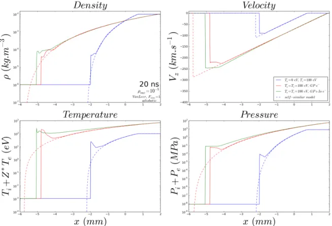
The work I present in this manuscript is represented schematically in fig.1.1. Omitted in this schema are the first part of chapter II where the bi-temperature magnetohydrody-namic (MHD) model is derived (2) and the GORGON code is presented (2.4). Also omit-ted is chapter III (3) which can be considered as a (very) small review of the physics of laser-solid-plasma interaction at, what could called "hydrodynamic" intensities. These intensities correspond to regimes such that the distribution functions (a notion defined in chapter II) are not departing "too far" from the maxwellian distribution under the laser action. In the last part of this chapter, emphasis is placed on the dynamic of the plasma plume generated by the laser and expanding away from the solid target. A review of the well-known one-dimensional, self-similar adiabatic and isothermal expansions is given, as well as an original (but preliminary) treatment of the hypersonic regions of the plume by using a solution of the inviscid Burger’s equation (i.e the "pressureless" Euler
equa-tion). In chapter IV (4) we introduce the topic of supersonic/hypersonic jets by studying both theoretically and numerically some fundamental properties of these objects. To do so, we use an idealized numerical setup where the jet enters, using boundary conditions, one side of the simulation domain which is filled with a background composed of plasma or/and magnetic field. We address especially the aspect of the stability of these jets by looking at the potentially disruptive effect of the Kelvin-Helmholtz instability and the sta-bilizing effect of the magnetic field. The chapter ends with the case of a supersonic jet propagating in a magnetized vacuum. We show that this configuration is extremely sta-ble and represents the perfect introduction for the fifth chapter. Indeed, in chapter V (5) we present an in-depth study of the production, in the laboratory, of magnetically colli-mated jets. The "source" of the jet in this setup the laser-produced plasma expanding in front of a solid target. In the following chapter VI (6) we address, both experimentally et numerically, the potential possibility to introduce variability in the source of the jets by adding a second pulse to the previous setup. In particular we vary the delay between the two pulses and observe the resulting changes in the internal structures of the collimated flow. In chapter VII (7) we investigate the case where the magnetic field is rotated by 90° such that it is parallel to the target surface. We show, strongly supported by experimental results, that the magnetic field action on the plasma dynamic results in the formation of what can be identified as magnetic slabs or "magnetic pancakes". It is also shown that these pancakes are largely structured by MHD instabilities. We suggest the potential in-terest of this configuration in the context of magnetic structuring of stellar atmospheres. Finally, in chapter VIII (8) and IX (9) we treat the topic that should be considered as been the "raison d’être" of this thesis, that is the three-dimensional study of magnetized ac-cretion dynamic in the laboratory. The setup makes use of the previously studied jets in order to use them as "accretion columns" impacting on solid obstacles. First are pre-sented briefly some very recent experimental results obtained at the LULI laboratory and then we expand the study using our 3D simulations to infer several fundamental features present in this type of experiment. In particular, we look at the asymmetric aspects of the developed structures as well as the importance correctly modeling the column-obstacle interaction. We highlight an important characteristic of the laboratory accretion shocks: the shock/postshock region itself is in a non equilibrium state with ions much hotter than electrons. This last point is a fundamental difference with the astrophysical case where the postshock equilibration times are sufficiently small to consider equals temperatures for electrons and ions. In addition to these chapters forming the core of this manuscript, we give in appendix a certain number of theoretical derivations of propagating modes and instabilities in several configurations. We notably derive the dispersion relations for modes propagating in magnetic interfaces or magnetic slabs. These derivations are not essential for the understanding of the core chapters.
1.4 Bibliography
[1] T.R. Kallman and P. Palmeri. Atomic data for x-ray astrophysics. Reviews of Modern Physics, 79:79–133, January 2007. 2
[2] E. Herbst and E.F. van Dishoeck. Complex Organic Interstellar Molecules. araa, 47:427–480, September 2009. 2
[4] Adelberger et al. Solar fusion cross sections. II. The pp chain and CNO cycles. Reviews of Modern Physics, 83:195–246, January 2011.2
[5] Elena Aprile and Stefano Profumo. Focus on dark matter and particle physics. New Journal of Physics, 11(10):105002, 2009.2
[6] C. N. Matthews and R. D. Minard. Hydrogen cyanide polymers, comets and the origin of life. Faraday Discussions, 133:393, 2006. 2
[7] Michel Nuevo, Stefanie N Milam, Scott A Sandford, Jamie E Elsila, and Jason P Dworkin. Formation of uracil from the ultraviolet photo-irradiation of pyrimidine in pure h2o ices. Astrobiology, 9(7):683–695, 2009.2
[8] Emeric Falize, Serge Bouquet, and Claire Michaut. Radiation hydrodynamics scal-ing laws in high energy density physics and laboratory astrophysics. In Journal of Physics: Conference Series, volume 112, page 042016. IOP Publishing, 2008.3
[9] DD Ryutov, RP Drake, and BA Remington. Criteria for scaled laboratory simula-tions of astrophysical mhd phenomena. The Astrophysical Journal Supplement Se-ries, 127(2):465, 2000. 3
[10] A. Frank, T. P. Ray, S. Cabrit, P. Hartigan, H. G. Arce, F. Bacciotti, J. Bally, M. Benisty, J. Eislöffel, M. Güdel, S. Lebedev, B. Nisini, and A. Raga. Jets and Outflows from Star to Cloud: Observations Confront Theory. Protostars and Planets VI, pages 451–474, 2014. 3
[11] J. Kwan and E. Tademaru. Jets from T Tauri stars - Spectroscopic evidence and colli-mation mechanism. ApJL, 332:L41–L44, September 1988.
[12] S. V. Lebedev, A. Ciardi, D. J. Ampleford, S. N. Bland, S. C. Bott, J. P. Chittenden, G. N. Hall, J. Rapley, C. A. Jennings, A. Frank, E. G. Blackman, and T. Lery. Magnetic tower outflows from a radial wire array Z-pinch. mnras, 361:97–108, July 2005. 3
[13] A. Ciardi, S. V. Lebedev, A. Frank, E. G. Blackman, D. J. Ampleford, C. A. Jennings, J. P. Chittenden, T. Lery, S. N. Bland, S. C. Bott, G. N. Hall, J. Rapley, F. A. S. Vidal, and A. Marocchino. 3D MHD Simulations of Laboratory Plasma Jets. apss, 307:17–22, January 2007.3
[14] D. Lynden-Bell. Magnetic collimation by accretion discs of quasars and stars. mnras, 279:389–401, March 1996.3
[15] P. M. Bellan, S. You, and S. C. Hsu. Simulating Astrophysical Jets in Laboratory Ex-periments. apss, 298:203–209, July 2005.3
[16] S. C. Hsu and P. M. Bellan. On the jets, kinks, and spheromaks formed by a planar magnetized coaxial gun. Physics of Plasmas, 12(3):032103, March 2005.3
[17] B. Albertazzi, A. Ciardi, M. Nakatsutsumi, T. Vinci, J. Béard, R. Bonito, J. Billette, M. Borghesi, Z. Burkley, S. N. Chen, T. E. Cowan, T. Herrmannsdörfer, D. P. Higginson, F. Kroll, S. A. Pikuz, K. Naughton, L. Romagnani, C. Riconda, G. Revet, R. Riquier, H.-P. Schlenvoigt, I. Yu. Skobelev, A.Ya. Faenov, A. Soloviev, M. Huarte-Espinosa, A. Frank, O. Portugall, H. Pépin, and J. Fuchs. Laboratory formation of a scaled protostellar jet by coaligned poloidal magnetic field. Science, 346(6207):325–328, 2014.3
[18] A. Ciardi, T. Vinci, J. Fuchs, B. Albertazzi, C. Riconda, H. Pépin, and O. Portugall. Phys. Rev. Lett., 110:025002, 2013. 3
[19] B Albertazzi, J Béard, A Ciardi, T Vinci, J Albrecht, J Billette, T Burris-Mog, SN Chen, D Da Silva, S Dittrich, et al. Production of large volume, strongly magnetized laser-produced plasmas by use of pulsed external magnetic fields. Review of Scientific Instruments, 84(4):043505, 2013. 3
[20] B Rus, K Rohlena, J Skála, B Králiková, K Jungwirth, J Ullschmied, KJ Witte, and H Baumhacker. New high-power laser facility pals—prospects for laser–plasma re-search. Laser and Particle Beams, 17(2):179–194, 1999. 4
[21] SV Lebedev, DJ Ampleford, SN Bland, SC Bott, JP Chittenden, J Goyer, C Jennings, MG Haines, GN Hall, DA Hammer, et al. Physics of wire array z-pinch implosions: experiments at imperial college. Plasma physics and controlled fusion, 47(5A):A91, 2005. 4
MagnetoHydroDynamic
Sommaire
2.1 Introduction . . . 10
2.2 Fluid equations from the kinetic theory . . . 12
2.2.1 Zero-order moment: the mass conservation equation . . . 12
2.2.2 First-order moment: the momentum conservation equation . . . . 13
2.2.3 Second-order moment: the energy conservation equation. . . 16
2.3 MagnetoHydroDynamic (MHD) reduction . . . 16
2.3.1 Summary of the multi-species fluid equations . . . 16
2.3.2 Expression of the collisional heating term . . . 18
2.3.3 The conservation energy for multi-species fluid equations . . . 19
2.3.4 The bi-temperature MHD model . . . 20
2.3.5 MHD mass conservation equation . . . 21
2.3.6 MHD momentum conservation equation . . . 21
2.3.7 MHD internal energy conservation equation. . . 24
2.3.8 The generalized Ohm’s law . . . 25
2.3.9 The displacement current in the Maxwell-Ampere equation . . . . 30
2.3.10 Relative importance of the various electric field terms in the gener-alized Ohm’s law . . . 31
2.3.11 The induction equation . . . 35
2.3.12 The quasi-neutrality assumption . . . 36
2.3.13 Conservation of the total energy in the MHD model . . . 36
2.4 The GORGON 3D resistive, bi-temperature MHD code . . . 39
2.4.1 Introduction . . . 39
2.4.2 Implemented equations . . . 40
2.4.3 Localization of the physical quantities in the GORGON grid . . . 40
2.5 Implementation of a laser module in the GORGON code . . . 41
2.5.1 Introduction . . . 41
2.5.2 Electromagnetic Wave propagation equation in a (unmagnetized) plasma . . . 42
2.5.3 Effect of electron-ion collisions on the propagation of light waves
in homogeneous plasmas . . . 45
2.5.4 Geometric optic approximation and the eikonal equation . . . 46
2.5.5 Implementing the laser deposition module in the three-dimensional, resistive MHD code GORGON . . . 47
2.5.6 Validation test for the laser module . . . 50
2.6 Implementation of the Biermann battery effect in the GORGON code . . 52
2.6.1 General description . . . 52
2.6.2 Details of the numerical implementation. . . 53
2.6.3 Simulation tests. . . 54
2.1 Introduction
In this chapter we present in details the MHD model and code that are the foundation of the work presented in the manuscript. The MHD model equations are derived from first principle, and although the model is well established and the derivation can be found in many excellent books, we have taken particular care to highlight and critically discuss the many assumption that are often made and somewhat overlooked.
In section2.2we derive the general fluid equations from the kinetic description. The central mathematical object in the kinetic theory of gas/plasmas is the distribution func-tion, noted f (r, v, t ). This function corresponds to the (most probable) number of parti-cles located, at a time t , in a infinitesimal volume d r3d v3(d r3= d xd yd z and d v3= vxvyvz
in Cartesian coordinates) of the phase space around the point (r, v). We will use the defi-nition for the number density of particle n(r, t ):
n(r, t ) = Ñ
v
f (r, v, t )d v3 (2.1)
Depending on whether collisions are taken into account or not, the equation describ-ing the evolution of the distribution function is the Vlasov equation (no collisions) or the Boltzmann equation (with collisions). The Boltzmann equation is written as:
∂f
∂t + (v · ∇) f + (a · ∇v) f = ˙fc (2.2) where a is the acceleration, ∇vis nabla operator applied in the velocity space and ˙fc
is the term representing the effect of collisions, both intra-species and inter-species. The formulation of this term is generally the trickiest part of the Boltzmann equation and sev-eral models exist, one of the most widely used is the Fokker-Planck (FP) equation. The collisionless Vlasov equation is obtained by setting ˙fc = 0 in 2.2(see [1] for a complete
derivation and discussion about this equation). The fluid equations, namely the equa-tions describing the conservation of mass, of momentum and of energy are obtained from the Boltzmann equation2.2by expressing the first three moments of the distribu-tion funcdistribu-tion (relative to the variable v). The process by which we obtain these equadistribu-tions is called a "reduction" because of the fact that the system is simplified and described in somewhat less details. Indeed, when integrating on the velocities v we loose for exam-ple all the details about the individual particles speeds which are replaced instead by the mean fluid velocity u:
n(r, t )u(r, t ) = Ñ
v
v f (r, v, t )d v3 (2.3)
The relation2.3is the 1th-order moment of the distribution function whereas2.1is its 0th-order moment. Once the mean velocity (i.e. the fluid velocity) defined, it is useful to introduce the velocity of the particle w in the frame of the fluid velocity u:
w = v − u (2.4)
In the vast majority of fluid models, a last third moment is also used and it is obtained by multiplying the Boltzmann equation2.2by mvv and then by integrating over all veloci-ties. As we shall see (see2.20), this new equation introduces, when using2.4, the pressure tensor ¯¯P defined by:
¯¯P =Ñ
v
mαww f (r, v, t )d v3 (2.5) where we introduced the mass mα of a particle of the specieα (electrons, ions...). It is important to note that, in general, the pressure is not a scalar but indeed a tensor de-scribed by the dyadic product ww in2.5. As we shall see, each equation describing the evolution of a moment involves the knowledge of the next moment of higher order. Thus, ideally, a fourth moment equation (describing the evolution of the heat flux) of the Boltz-mann equation would be necessary to express the evolution of the pressure tensor and then a fifth moment equation would be necessary to express the evolution of this fourth moment and so on... Even if some models have been developed to include such higher orders moments equations ([2]), the vast majority of fluid descriptions use only the first three conservation equations and replace the lacking equations by what is called a clo-sure relation. There are two different types of fluid cloclo-sure schemes. The truncation schemes, where higher order moments are assumed negligible or simply prescribed in terms of lower moments (see [3]), and the asymptotic schemes where assumptions on certain dimensionless parameters allows to infer, from the kinetic theory, expressions for the higher moments involved. For example, the Chapman-Enskog theory of a neutral gas dominated by collisions allows to find simplified expressions for the transport coeffi-cients, see [4]). The description of a complete physical system by the fluid equations will be increasingly precise as the distribution function tends toward a function well described by a decreasing number of moments. The general idea behind is that, to keep the exact same degree of informations between the kinetic description and the fluid description, one would need to compute the evolution of an infinite number of moments. It turns out that in many cases of interest, the distribution function is "simple enough" to be relatively well characterized by a small number of moments. The best example is of course the one temperature Maxwell–Boltzmann distribution:
f (r, v, t ) = n(r, t ) µ mα 2πkBT ¶3/2 exp µ −mα(v − u) 2 2kBT ¶ (2.6) This distribution function is, as one can see, completely described by the first three moments, namely the density, the mean velocity and the temperature. The Maxwell–Boltzmann distribution is thus the "perfect" function in the framework of the three-moments fluid model. As is well known, it can be shown [4–6] that, in the limit of a collision dominated system (large term ˙fc), the Boltzmann equation2.2drives the distribution function
to-wards a Maxwell–Boltzmann distribution2.6. This "relaxation" process is a direct result of the H-theorem of Boltzmann [7]. Therefore, a fluid model will always be more adapted for collisional plasmas (such that the mean free path of a particle is much smaller than the typical size of the system) than for weakly or non-collisional plasmas where the Vlasov equation is required.
In section2.3we present an additional simplification to the system of fluid equations obtained in section2.2. Indeed, the system of equations derived from the moments of the Boltzmann equation (see section2.2) have to be applied to each speciesα of the plasma. For each species, the fluid model requires the solution of five equations (one for the mass conservation, three for the momentum conservation and one for the energy conserva-tion). So if Nαis the number of different species composing the plasma, the total number of fluid equations is 5Nα, plus the coupled eight maxwell equations. This is a mathemati-cally very demanding system and we highlight the fact that Nαcan be very large. Since the
electromagnetic forces depend on the charge state, each ionization state of a given specie needs to be treated separately. The so-called "MHD reduction" that will be described, basically replaces all the different "fluids" by one neutral fluid. One central assumption, among others, is that the time scales of interests are sufficiently large compared to the time scale where charge separation occurs. In such case the net charge density in the plasma can then be set to zero. We will first reduce all ion charge states to a single "heavy" fluid with a mean degree of ionization Z∗i and then the reduction will be applied the elec-tron (light) and ion (heavy) fluid mass and momentum conservation equations, thus re-ducing the system to 2 + Nαequations.
The remainder of the chapter (section2.4) will be dedicated to a detailed description of the model used in the code GORGON, which is somewhat a further reduction of the MHD model given in section2.3, and the implementation of several new physics modules (laser depostion, Biermann battery ,...).
2.2 Fluid equations from the kinetic theory
2.2.1 Zero-order moment: the mass conservation equation
As explained in the introductory section2.1, the starting point to derive the fluid equa-tions is the Boltzmann equation2.2. The zero-order moment is obtained by directly inte-grating this equation over the velocities:
∂ ∂t Ñ v f d v3 + Ñ v (v · ∇)f dv3+ Ñ v (a · ∇v) f d v3= δn δt ¯ ¯ ¯ ¯ c (2.7) where the right-hand side (RHS),
δn δt ¯ ¯ ¯ ¯ c = Ñ v ˙ fcd v3 (2.8)
corresponds to a source term describing, for example, an external injection of matter or nuclear reactions (through collisions). The first term on the left-hand side (LHS) is simply, using2.1, equal to the partial time derivative of the number density:
∂ ∂t Ñ v f d v3 = ∂n ∂t (2.9)
The second term in LHS can be easily rewritten by noticing that the gradient applies only to the variable r: (v · ∇)f = ∇ · (vf ), and that the integration is only over the velocities, the gradient can then be removed from the integrals to give:
Ñ v (v · ∇)f dv3= ∇ · Ñ v v f d v3 = ∇ · (nu) (2.10)
where we used relation2.3. This terms corresponds to the divergence of the mass flux. For the last term of the LHS, we need to explicit the expression of the acceleration a. We consider the general case of the Lorentz force Florentz= FE+FB= qE+qv×B where E is the
local electric field, B the local magnetic field and q the electric charge of the particle. The electric force does not depend on the velocity and the magnetic force has the particularity
that its component FBi (i=x,y,z) does not depend on the velocity vi. The acceleration is
related to the force by the Newton’s second law: a = Florentz/m. Using the index notation
(summation over all indices i ), we can thus write: Ñ v (a · ∇v) f d v3= Ï vj 6=i ai Z vi ∂vif d vi d v2= Ï vj 6=i ai£ f ¤vvii=+∞=−∞d v2= 0 (2.11)
where we used the justifiable assumption that the distribution function vanish for vi=
±∞ and thus£ f ¤vvii=+∞=−∞= 0. Injecting expressions2.9,2.10and2.11into2.7we get the first fluid equation: ∂n ∂t + ∇ · (nu) = δn δt ¯ ¯ ¯ ¯ c (2.12) This equation describes the conservation of the quantity of matter or, equivalently by multiplying it by the particle mass m, the conservation of mass.
2.2.2 First-order moment: the momentum conservation equation
The second fluid equation is obtained first multiplying the Boltzmann equation2.2by the particle momentum mv and then by integrating over the velocities:
∂ ∂t Ñ v mv f d v3 + Ñ v mv(v · ∇)f dv3+ Ñ v mv(a · ∇v) f d v3= A (2.13) where: A = Ñ v mv ˙fcd v3 (2.14)
The first term in the LHS of equation2.13is, using2.3, simply equal to: ∂ ∂t Ñ v mv f d v3 = ∂(ρu) ∂t (2.15)
whereρ = mn is the mass density. The i component of the second term of the LHS can be rewritten using the same argument as for the zero-order moment (i.e. the gradient applies only on r): Ñ v mv(v · ∇)f dv3 ¯ ¯ ¯ ¯ ¯ ¯ i =∂j Ñ v mvivjf d v3 (2.16)
We can go further by using the previously defined (see2.4) centered velocity w, for which we recall the expression:
w = v − u (2.17) with, by definition: Ñ v w f d v3= Ñ v (v − u) f dv3= nu − nu = 0 (2.18)
Inserting the central moment2.17in2.16we get: Ñ v mv(v · ∇)f dv3 ¯ ¯ ¯ ¯ ¯ ¯ i =∂j Ñ v m(wiwj+ ujwi+ uiwj+ uiuj) f d v3 (2.19)
the first integral in the RHS of2.19defines the kinetic pressure tensor ¯¯P: ¯¯
Pi j=
Ñ
w
mwiwjf d w3 (2.20)
where we used the fact that d v3= d w3and the integration bounds are still ±∞ for each component of the central moment w. The second and third integral of the RHS in2.19are zero because of the definition of the central moment2.18:
Ñ v mujwif d v3= muj Ï wk6=i Z wi wif d wi d w2= 0 (2.21) and Ñ v mujwif d v3= mui Ï wk6=j Z wj wjf d wj d w 2 = 0 (2.22)
Finally the third term on the RHS of2.19is simply given by:
∂j Ñ v muiujf d v3
=∂j(ρuiuj) =ρ(uj∂j)ui+ ui∂j(ρuj) (2.23) then, by inserting all terms2.20,2.21,2.22and2.23in2.19we get:
Ñ
v
mv(v · ∇)f dv3= ∇ · ¯¯P + ρ(u · ∇)u + u(∇ · (ρu)) (2.24) and by summing the first (2.15) and second term (2.24) of the first-order moment equation2.13we find: ∂ ∂t Ñ v mv f d v3 + Ñ v mv(v · ∇)f dv3=ρd u d t + ∇ ·¯¯P +mu δ n δt ¯ ¯ ¯ ¯ c (2.25) where d u/d t =∂u/∂t + (u · ∇)u is the Lagrangian (or total) derivative and where we used the first fluid equation2.12.
Now we derive the expression of the third term of the LHS of2.13. We use again the fact that a component ai of the particle acceleration does not depend on the component
vi of the particle velocity. We can thus write:
Ñ v mv(a · ∇v) f d v3 ¯ ¯ ¯ ¯ ¯ ¯ i = Ñ v mvi∂vj(ajf )d v 3 (2.26)
Ñ v mvi∂vi(aif )d v 3= Ï vj6=vi mai Z vi vi∂vif d v2 (2.27) and with: Z vi vi∂vif = [vif ] vi=+∞ vi=−∞− Z vi f d vi= − Z vi f d vi (2.28) we have Ñ v mvi∂vi(aif )d v 3 = − Ï vj6=vi mai Z vi f d vi d v2 (2.29)
using the index notation, we can write the particle acceleration as: ai=
q mEi+
q
m²i j kvjBk (2.30)
and inserting2.30in2.29we get:
− Ï vj6=vi mai Z vi f d vi d v2= −qEi Ñ v f d v3− q²i j kBk Ñ v vjf d v3 (2.31)
An finally, using2.1and2.3, we obtain: Ñ
v
mvi∂vi(aif )d v
3
= −qnEi− qnuiBi (2.32)
If we now suppose that in relation2.26we have j 6= i the result in simply:
Ñ v mvi∂vj(ajf )d v 3 = Ï vk6=vj majvi Z vj ∂vjf d vj d v 2 = 0 (2.33)
because the distribution function is zero for v = ±∞. We can finally express the third term in the LHS of equation2.13as
Ñ
v
mv(a · ∇v) f d v3= −qnE − qnu × B (2.34)
and assembling all the term of the first-order moment equation (2.25and2.34we find the second fluid equation:
ρd u d t = −∇ · ¯¯P + qnE + qnu × B + A − mu δn δt ¯ ¯ ¯ ¯ c (2.35)
2.2.3 Second-order moment: the energy conservation equation
By multiplying the Boltzmann equation2.2by vv (the dyadic product) one would obtain the equation describing the evolution of the pressure tensor ¯¯P and involving the heat flux tensor ¯¯QT(tensor of order 3) defined by:
¯¯ QT=
Ñ
w
mwww f d w3 (2.36)
This equation is quite complicated and not very useful since almost never used in this form. The process to obtain it is however very similar to the one used for the two previous moments. Here we present a simplified form obtained under the assumption that the heat flux can be expressed as a vector defined by:
q = 1 2
Ñ
w
mw2w f d w3 (2.37)
and valid if the velocity anisotropies are small. If furthermore the non-diagonal terms of the pressure tensor are also neglected (also true for small anisotropies) then the pres-sure can be simplified as:
p =1 3 Ñ w mw2f d w3=1 3Tr ( ¯¯P) (2.38)
where Tr ( ¯¯P) is the trace of the pressure tensor. In this case, equation obtained from the second-order moment can be written:
∂ ∂t µ 3 2p + 1 2ρu 2 ¶ + ∇ · · q +µ 5 2p + 1 2ρu 2 ¶ u ¸ = qnu · E + K − u · A +1 2mu 2δn δt ¯ ¯ ¯ ¯ c (2.39) where: K = Ñ v mv2 2 f˙cd v 3 (2.40)
With the internal energy density defined as² = p/(γ − 1) we clearly see that equation 2.39corresponds to the energy fluid equation for a population with an adiabatic index γ = 5/3.
2.3 MagnetoHydroDynamic (MHD) reduction
2.3.1 Summary of the multi-species fluid equations
We now derive the complete MHD model with, as starting point the multi fluid equations derived in the previous section. In the following, the indexα is used to identify a given population (electrons, ions).
I) The conservation of matter, obtained by multiplying equation2.12by mα: ∂ρα
∂t + ∇ · (ραu) = Sα (2.41)
where S is a source term (nuclear reactions, external source...). We can write this equation using the the lagrangian derivative d /d t =∂/∂t + uα· ∇:
dρα
d t = −ρα∇ · uα (2.42)
II) The conservation of momentum (from2.35): ρα µ ∂uα ∂t + (uα· ∇)uα ¶ = −∇pα+ qαnαE + qαnαuα× B + Rα− mαuαS (2.43)
where Rαis the friction force applying on the populationα and we considered the re-duction of the pressure tensor as a scalar (valid if the time between two collisions is much smaller than the time needed by a particle to make a complete magnetized gyration).
III) The conservation of internal energy: ∂²α
∂t + ∇ · (²αuα) = −pα∇ · uα− ∇ · qα+ Q
c
α+ Hα (2.44)
where Qcα is the heat transfer because of collisions and Hα is a energy source term (laser heating...). We also have the important relation:
X α Q c α+ X α uα· Rα= 0 (2.45)
This last equality, contrary to what one might think, does not mean that Qαc = −uα· Rα.
This is because the frictional heating is only one component of the total heating Qcαdue to the collisions (see2.3.2for more details).
IV) Maxwell’s equations also need to be included in the system to describe the time evolution of the electromagnetic fields:
∇ · E =ρq ²0 (2.46) ∇ · B = 0 (2.47) ∂B ∂t = −∇ × E (2.48) ∇ × B = µ0j + 1 c2 ∂E ∂t (2.49)
withρqthe net charge density and:
ρq=
X
α qαnα (2.50)
j the electrical current obtained from sum of the currents of each population: j =X
α qαnαuα (2.51)
and²0is the vacuum permittivity whereasµ0is the vacuum permeability.
In writing all the equations2.41-2.51we get a very complex system of equations where the only assumption having been made concerns basically the fact that the distribution function for each species, fα, can be relatively well described by the first three moments. Which is generally valid when the mean free path of the particles is much smaller than the characteristic size of the system because in this case the distribution function tends towards a Maxwellian.
2.3.2 Expression of the collisional heating term
Frictional heating
In equation2.44we have introduced the term Qαc where several different terms are "hid-den". First, the work of the frictional forces Rαacting on each populationα is the source of heat production (conversion of ordered kinetic energy into thermal energy). A simple way to describe how this heating is distributed among each component of the plasma has been given by Woods [8]. Let us suppose that the populationα is heated, because of a fric-tional force with the populationβ, at rate φα←β, and similarly for the populationβ. Then we have:
QFr i c=φα←β+ φβ←α= −uα· Rα− uβ· Rβ (2.52)
where QFr i cis the total frictional heating in the plasma. By virtue of the Newton’s third
law (action-reaction law), the frictional momentum transfer fromα to β must be equal to the opposite of the momentum transfer fromβ to α, that is: Rα= −Rβ. With this relation
we can write the total frictional heating2.52as:
QFr i c= Rα· (uβ− uα) = Rβ· (uα− uβ) (2.53)
It is now necessary to determine how this total frictional heating is distributed among the populations. The simplest way, is to consider the case of isotropic elastic collisions where the energy after a collisionα/β is distributed inversely to the particle masses:
φα←β φβ←α= mβ mα (2.54) Inserting2.54in2.52we find: φα←β= mβ mα+ mβQFr i c (2.55)
For example, for ions with mass miand electrons with mass me<< mi, it is easy to see
that the frictional heating will go mainly into the lightest population, that is, the electrons. This is the reason why, in many two-temperature (MHD) models, the frictional heating is neglected for the ions.
Thermal equilibration
Another important term included in the heating Qcαis related to the fact that if two dif-ferent populations, say electrons and ions, have difdif-ferent temperatures (Te 6= Ti) then,
because of collisions, they will tend to "correct" this deviation on a time scale of the order of the time between two collisions (or equivalently on a spatial scale of the order of the mean free path). The expression for this thermal equilibration process (first derived by Landau in 1937 [9]) is given by:
Qei = −3
me
mi
neνeikB(Te− Ti) (2.56)
whereνei is the electron-ion collision frequency [10]. We shall refer to Qei as the rate
of heat exchange from electrons toward ions and note that the relation Qei = −Qi eholds.
In summary, using eq.2.53,2.55,2.56, and the fact that Ri= −Re, the collisional heating
Qce= mi me+ mi Re· (ui− ue) − 3 me mi neνeikB(Te− Ti) (2.57) Qci = me me+ mi Re· (ui− ue) + 3 me mi neνeikB(Te− Ti) (2.58)
2.3.3 The conservation energy for multi-species fluid equations
The system of fluid equations summarized in2.3.1is completely self-consistent in terms of energy conservation. It can be seen by, first, identifying all forms of energy:
1. Kinetic energy:²ki n= 1/2ρu2 2. Internal energy:²
3. Electromagnetic energy:²EM=²0E2/2 + B2/2µ0
For each form of energy, there is a corresponding conservation equation. The internal energy conservation equation has already been derived (see eq.2.44), the conservation of kinetic energy is obtained by multiplying the momentum equation2.43by uα, and finally, the conservation of electromagnetic energy (Poynting’s theorem) is obtained by multiply-ing eq.2.48by B and then using eq.2.49. The system of equations is then given by:
Energy Conservation equation
Kinetic ∂² ki n α ∂t + ∇ · (² ki n α uα) = −uα· ∇ · pα+ qαnαuα· E + uα· Rα Internal ∂²α ∂t + ∇ · (²αuα) = −pα∇ · uα− ∇ · qα+ Q c α+ Hα Electromagnetic ∂² EM ∂t + ∇ · µ E × B µ0 ¶ = −E · j
The RHS of the kinetic equation is composed of three terms: the work of pressure forces, the work of the electric field (no work from the magnetic field) and the work of the frictional force. The RHS of the internal equation is composed of the compressional term, the heat transfer term, the frictional heating term as well as all possible external source terms (laser, radiative emission...). Concerning the electromagnetic energy, the "trans-port" term ΠEM= E × B/µ0is the Poynting vector and represents the directional energy
flux density (W.m−2) of the electromagnetic field. The RHS of this equation represents the electromagnetic energy losses/gains realized through the work the electric field is do-ing on the fluid particles. The conservation of the total energy is given by the sum of the three conservation equations, for all the speciesα composing the plasma:
∂²t ot ∂t + ∇ · µ ΠEM+ X α h³ ²ki n α + ²α+ pα ´ uα+ qα i¶ =X α Hα (2.59)
where we have used relation2.45as well as relation2.51to writeP
αqαnαuα·E = j·E and
²t ot is the total energy density:
²t ot=²EM +X α ³ ²ki n α + ²α ´ (2.60)
Equation2.60describes the strict conservation of the total energy. It can be seen that in the absence of external heating (P
αHα= 0) the total energy is only transported with the
flux: Ftot=ΠEM+ X α h³ ²ki n α + ²α+ pα ´ uα+ qα i (2.61) This flux can also be written in terms of the enthalpy density hαof each speciesα:
hα=²α+ pα (2.62) giving: Ftot=ΠEM+ X α h³ ²ki n α + hα ´ uα+ qα i (2.63) The reason for discussing in some details the conservation of total energy is because it will be, when deriving the MHD model in the next section, particularly important when interpreting the meaning of what we shall call the "MHD energy".
2.3.4 The bi-temperature MHD model
The first step to derive the full system of equation is to consider the plasma to be com-posed of electrons (α = e) of mass me and charge qe = −e and only one species of ion
(α = i) of mass mi and charge qi= eZ∗, where Z∗is the average degree of ionization. Both
of these species obey equations2.41-2.43-2.44and are coupled with the Maxwell’s equa-tions2.46-2.47-2.48-2.49.
We first define the total mass density of the plasma:
ρ = mene+ mini =ρe+ ρi (2.64)
then the velocity u of the center of mass of the plasma:
ρu = ρeue+ ρiui (2.65)
and the total electrical current density:
j = eZ∗niui− eneue (2.66)
From2.65and2.66we can write ueand uias functions of u and j:
ui= ρ ρ∗u + me eρ∗j (2.67) ue= Z∗ni ne ρ ρ∗u − ni ne mi eρ∗j (2.68) where: ρ∗=ρ i+ Z∗ni ne ρe (2.69)
We see that up to this point, we have made no extra assumptions compared to the multi-species system described previously; we are just adding or averaging the previous quantities. We shall make further assumptions on spatial or temporal scales, as late as possible in our MHD derivation.
2.3.5 MHD mass conservation equation
As in the case of the multi-species fluid system, the first MHD equation describes the conservation of the "MHD mass density". It is obtained by directly summing the mass conservation equation for both species2.41:
∂(ρe+ ρi)
∂t + ∇ · (ρeue+ ρiui) = 0 (2.70) and, using,2.64 2.65:
∂ρ
∂t + ∇ · (ρu) = 0 (2.71)
Equation2.71is the conservation equation for the mass density of the reduced MHD single-fluid.
2.3.6 MHD momentum conservation equation
An equation for the single-fluid momentum can be obtained from:
d (ρu) d t =ρ d u d t + u dρ d t = d (ρeue) d t + d (ρiui) d t =ρe d ue d t + ρi d ui d t + ue dρe d t + ui dρi d t (2.72) and thus: ρd u d t =ρe d ue d t + ρi d ui d t + dρe d t (ue− u) + dρi d t (ui− u) (2.73)
From now, one has to be very cautious by the meaning of the total derivative d /d t used in the previous equations. Indeed, when writing these equations we have considered the problem in the frame of the velocity u of the center of mass defined by2.65. Thus we have the important relation:
d d t =
∂
∂t+ (u · ∇) (2.74)
This precision is important because we can’t just insert directly the electron and ion momentum equations (given by2.43) in2.73since with our notation:
d ui
d t 6= ∂ui
∂t + (ui· ∇)ui (2.75)
and same for electrons. As we will see, the problem will be easily solved using the ex-pressions for the electron and ion velocities2.68and2.67provided the plasma is assumed to be neutral (see below).
Before to treat this problem, let’s look at the last two terms of the RHS of equation2.73 which can be rewritten using the expressions for the electron and ion velocity in terms of single-fluid velocity and electrical current density (eq.2.67and2.68):
dρe d t (ue− u) = · Z∗niρ − neρ∗ neρ∗ u − ni ne mi eρ∗j ¸ dρe d t (2.76) dρi d t (ui− u) = ·ρ − ρ∗ ρ∗ u + me eρ∗j ¸ dρi d t (2.77)
From here, we clearly see that it is impossible to remove all the dependencies in neand
niwithout additional assumption. The terms in eq.2.76and2.77are corrective terms that
take into account the fact that the single-fluid velocity is not equal to the velocity of both electrons and ions.
To proceed further, we make one of the main assumptions of the MHD model, namely that the single-fluid is considered as globally neutral. This is the quasi-neutrality of the plasma and it corresponds to the equality:
ne= Z∗ni (2.78)
The assumption quasi-neutrality of the plasma is strong, in the sense that it corre-sponds to the suppression of all physical processes related to charge separation. We will discuss in details the domain of validity of the MHD model, but let’s say for now that equation2.78acts as a sort of low-pass filter, by filtering all the dynamic occurring on the electron time scale (ω−1pe). With the assumption of quasi-neutrality (eq.2.78), we see from eq.2.69thatρ∗=ρe+ ρi=ρ and thus the sum of equations2.76and2.77leads to:
dρe d t (ue− u) + dρi d t (ui− u) = memi eρ j · d ni d t − 1 Z∗ d ne d t ¸ = −me eZ∗ ρi ρ d Z∗ d t j (2.79)
Furthermore, with our quasi-neutrality assumption, we can rewrite the electron (α = e, 2.68) and ion velocities (α = i,2.67) as:
uα= u + γαj (2.80)
where, from2.96and2.97, the factorsγαare given by: γe= − mi eZ∗ρ (2.81) γi= me eρ (2.82)
With these notations, the first two terms of the RHS of2.73writes: ραd uα d t =ρα µ ∂uα ∂t + (uα· ∇)uα ¶ − γαρα(j · ∇)uα (2.83)
In this expression we recognize in the first and second term of the RHS the "correct" (i.e. in the correct frame) lagrangian derivative given by equation2.43. Injecting these expressions and using the fact thatγeρe= −γiρiandγe−γi= −1/ene(from2.81and2.82),
the sum of eq.2.83of electrons and ions can be written as (with the term source S = 0): ρe d ue d t + ρi d ui d t = −∇(pe+ pi) + j × B − me e ρi ρ(j · ∇) µ j ene ¶ (2.84) In writing equation2.84we have used the definition of the total electrical current den-sity (eq.2.66), as well as the fact that Re= −Riby virtue of the Newton’s third law
(action-reaction law). This last point is specific to the MHD model: indeed, for the center of mass, the friction forces vanish. It is important to note that this is not related at all to the fact that the plasma has to be inviscid or infinitely conducting; as we shall see later, its just a consequence of the mathematical construction of the MHD reduction. Also, we see that the electric field has completely vanished as a consequence of the plasma neutrality (2.78)
Finally, by summing eq. 2.84and2.79, we can finally write the complete MHD mo-mentum equation (eq.2.73) as:
ρd u d t = −∇(pe+ pi) + j × B − me e ρi ρ · 1 Z∗ d Z∗ d t j + (j · ∇) µ j ene ¶¸ (2.85) Equation 2.85 is the most general MHD momentum equation of a bi-temperature plasma with non constant ionization. The last two terms in the RHS in this equation are often neglected in MHD models because they are proportional to me, the electron mass
and thus they are in some way a "reminiscence" of the fact that the MHD models includes the electron fluid equations. Let’s call the first of these term Fio:
Fio= − me e ρi ρ 1 Z∗ d Z∗ d t j (2.86)
In order to quantify the importance of this force we can first remark that this force is always directed perpendicular to the j×B force so these two component will not compete against each other. Therefore, to evaluate its importance we must instead make the com-parison with the pressure forces. Supposing that the characteristic time scale of ionization is given by electron-ion collisions, we can write d Z∗/d t ∼ Z∗νei (νei is the electron-ion
collision frequency) and then using the estimation j ∼ B/µ0L (L is the characteristic scale
of the macroscopic gradients, see2.129for details), we find: |∇(p)| |Fio| ∼ me e Lνeij p ∼ νei eB/me B2/µ0 p ≈ νei ωceβ −1 (2.87)
whereβ is the ratio of the magnetic pressure B2/2µ0to the thermal pressure p (here
p = pe+ pi is the total pressure). ωce = eB/meis the electron cyclotron frequency. Thus,
the "ionization" force will be negligible if: νei
ωce ¿ β
(2.88) One can see that if the plasma beta is close to unity then condition2.88is equivalent to say that the "ionization" force will be negligible if electrons are strongly magnetized. There is another case where this force is also negligible: if the energy density in the plasma is such that atoms are and remain fully ionized (as it is often the case in "HEDLA" plas-mas), then we simply have d Z∗/d t → 0 and therefore Fio→ 0. The second reminiscent
term that we will call the inertial force FIner:
FIner= − me e ρi ρ(j · ∇) µ j ene ¶ (2.89) This force, also almost always neglected, has been studied by other authors who have observed that it was needed in order to conserve the total energy in the MHD system (a question treated in this chapter, see2.3.13). They notably studied its effect on the Grad-Shafranov equation used to describes equilibrium state in a torus (see [11;12]). This force reflects the fact that electrons have actually a finite inertia. As we will see in the section concerning the derivation of the generalized Ohm’s law (2.3.8), this inertial force is associ-ated to an inertial electric field (as it is the case for "ionization" force). In order to facilitate this future link, we can note that the sum of the two non-trivial terms can be expressed (after "some" calculations):
FIo+ FIner= −∇ · µ me e ρi ρ jj ene ¶ (2.90)