Drought-induced regime shift and resilience of a Sahelian ecohydrosystem

HAL Id: hal-02344434

https://hal.archives-ouvertes.fr/hal-02344434

Submitted on 1 Jun 2021

HAL is a multi-disciplinary open access

archive for the deposit and dissemination of

sci-entific research documents, whether they are

pub-lished or not. The documents may come from

teaching and research institutions in France or

abroad, or from public or private research centers.

L’archive ouverte pluridisciplinaire HAL, est

destinée au dépôt et à la diffusion de documents

scientifiques de niveau recherche, publiés ou non,

émanant des établissements d’enseignement et de

recherche français ou étrangers, des laboratoires

publics ou privés.

Distributed under a Creative Commons Attribution| 4.0 International License

Drought-induced regime shift and resilience of a

Sahelian ecohydrosystem

Valentin Wendling, Christophe Peugeot, Ángeles Mayor, Pierre Hiernaux, Eric

Mougin, Manuela Grippa, Laurent Kergoat, Romain Walcker, Sylvie Galle,

Thierry Lebel

To cite this version:

Valentin Wendling, Christophe Peugeot, Ángeles Mayor, Pierre Hiernaux, Eric Mougin, et al..

Drought-induced regime shift and resilience of a Sahelian ecohydrosystem. Environmental Research

Letters, IOP Publishing, 2019, 14 (10), pp.105005. �10.1088/1748-9326/ab3dde�. �hal-02344434�

Drought-induced regime shift and resilience of a

Sahelian ecohydrosystem

To cite this article: Valentin Wendling et al 2019 Environ. Res. Lett. 14 105005

View the article online for updates and enhancements.

Recent citations

Impacts of climate and environmental changes on water resources: A multi-scale study based on Nakanbé nested watersheds in West African Sahel Y. Patrick Gbohoui et al

-Intermittent rivers and ephemeral streams: Perspectives for critical zone science and research on socioecosystems

Ophelie Fovet et al

-A dynamic land use/land cover input helps in picturing the Sahelian paradox: Assessing variability and attribution of changes in surface runoff in a Sahelian watershed

Roland Yonaba et al

Environ. Res. Lett. 14(2019) 105005 https://doi.org/10.1088/1748-9326/ab3dde

LETTER

Drought-induced regime shift and resilience of a Sahelian

ecohydrosystem

and Thierry Lebel5

1 _{Hydrosciences Montpellier(HSM), IRD, Univ. Montpellier, CNRS, Montpellier, France}

2 _{Copernicus Institute of Sustainable Development Géosciences Environnement, Utrecht Univ., Utrecht, Netherlands} 3 _{Géosciences Environnement Toulouse(GET), CNRS, IRD, UPS, Toulouse, France}

4 _{Laboratoire écologie fonctionnelle et environnement(ECOLAB), UPS, CNRS, Toulouse-INP, Toulouse, France} 5 _{Univ. Grenoble Alpes, CNRS, IRD, Grenoble INP, UMR IGE, Grenoble, France}

6 _{Author to whom any correspondence should be addressed.}

E-mail:valentin.wendling@ird.fr,christophe.peugeot@ird.fr,A.GarciaMayor@uu.nl,pierre.hiernaux2@orange.fr,

mouginbassignac@aol.com,manuela.grippa@get.omp.eu,laurent.kergoat@get.omp.eu,romain.walcker@univ-tlse3.fr,sylvie.galle@ ird.frandthierry.lebel@univ-grenoble-alpes.fr

Keywords: Sahel, eco-hydrology, alternative stable states, regime shifts, rainfall variability Supplementary material for this article is availableonline

Abstract

The Sahel

(a semi-arid fringe south of the Sahara) experienced a long and prolonged drought from the

1970s to the mid-1990s, with a few extremely severe episodes that strongly affected ecosystems and

societies. Long-term observations showed that surface runoff increased during this period, despite the

rainfall deficit. This paradox stems from the soil degradation that was induced by various factors,

either directly linked to the drought

(impact on vegetation cover), or, in places, to human practices

(land clearing and cropping). Surface runoff is still increasing throughout the region, suggesting that

Sahelian ecohydrosystems may have shifted to a new hydrological regime. In order to explore this

issue, we have developed a simple system dynamics model incorporating vegetation–hydrology

interactions and representing in a lumped way the

first order processes occurring at the hillslope scale

and the annual timestep. Long term observations on a pilot site in northern Mali were used to

constrain the model and define an ensemble of plausible simulations. The model successfully

reproduced the vegetation collapse and the runoff increase observed over the last 60 years. Our results

confirmed that the system presents two alternative states and that during the drought it shifted from a

high-vegetation/low-runoff regime to the alternative low-vegetation/high-runoff one, where it has

remained trapped until now. We showed that the mean annual rainfall deficit was sufficient to explain

the shift. According to the model, vegetation recovery and runoff reduction are possible in this system,

but the conditions in which they could occur remain uncertain as the model was only constrained by

observations over the collapse trajectory. The study shows that the system is also sensitive to the

interannual and decadal variability of rainfall, and that larger variability leads to higher runoff. Both

mean rainfall and rainfall variability may increase in central Sahel under climate change, leading to

antagonist effects on the system, which makes its resilience uncertain.

1. Introduction

Due to interactions between changing external forcing factors(e.g. rainfall) and internal dynamics, an envir-onmental system (e.g. a forest) may shift into new states where it stays even if the forcing factors return to

their initial value. In such a system, two alternative stable states may exist towards which the system is attracted (e.g. forest versus savannah, Staver et al

2011). For certain conditions, both equilibria can

coexist and the system can shift abruptly from one to the other when critical thresholds(or tipping points)

OPEN ACCESS RECEIVED

28 March 2019

REVISED

9 August 2019

ACCEPTED FOR PUBLICATION

22 August 2019

PUBLISHED

4 October 2019

Original content from this work may be used under the terms of theCreative Commons Attribution 3.0

licence.

Any further distribution of this work must maintain attribution to the author(s) and the title of the work, journal citation and DOI.

are passed(review in Scheffer et al2001). This kind of

behaviour has been widely studied in ecological systems(Scheffer and Carpenter2003, Rietkerk et al

2004, Hirota et al2011, van Nes et al2014, Yin et al

2014), among others. Attention has been also paid to

regime shifts in human societies driven by environ-mental factors(Di Baldassarre et al2013, Broderstad and Eythorsson2014, Sivapalan2015, Downey et al

2016, Kuil et al2016).

Global change might increase the potential for the tipping of some key elements of the Earth’s system (Lenton et al2008, Barnosky et al2012, Steffen et al

2018). Whilst the existence of tipping points at the

ple-natery scale(Brook et al2013) and their propagation

across scales(Hughes et al2013) is debated, examples

exist at the regional scale, such as the the collapse of the ‘green Sahara’ and the shrinking of Lake Chad around 6000 BP as a response to a gradual change in the Earth’s orbital parameters (Claussen et al1999).

Marked and persistent ecohydrological changes have been observed in the Sahel(a semi-arid belt south of the Sahara) over the past 60 years. This region experi-enced a severe and prolonged drought from the 1970s onwards(Lebel and Ali 2009), with extremely severe

episodes that have strongly and durably affected ecosys-tems and societies. Over most of the Sahel, greening has been observed by satellite imagery since the 1980s (Fensholt et al2012, Dardel et al2014). Concurrently,

long-term observations have shown that the outflow of Sahelian watersheds has increased from the 1950s onwards(Mahé and Paturel2009, Gardelle et al2010, Descroix et al2012, Gal et al2016), including during the

drought(the so-called ‘Sahelian paradox’; Favreau et al

2009). Field studies showed that these apparently

conflicting changes resulted from smaller scale, soil-dependent, processes. Vegetation(mainly herbaceous) recovered on deep sandy soils, driven by post-drought rainfall increase, whereas it decayed on shallow soils, despite the annual rainfall trend, causing erosion and runoff(Dardel et al2014, Trichon et al2018, Gal et al

2017). In some highly populated areas (e.g. South West

Niger), this so-called regreening was not observed due to the impact of human activities(land clearing, crops which are less green than rangelands, fertility losses; Favreau et al(2009), Hiernaux et al (2009).

As in other semi-arid regions, the Sahelian hydrol-ogy is strongly dependent on surface conditions(e.g. Casenave and Valentin1992, Peugeot et al1997). At

the elementary scale, heavy rains favour soil crusting all the more since the vegetation cover is sparse; a loss (gain) of vegetation cover favours (prevents) erosion and fertility losses, which in turn prevents(favours) vegetation expansion. These small-scale mechanisms combine into a positive feedback loop which has been shown to be involved in larger scale desertification dynamics (D’Odorico et al2013, Wilcox et al2017, Saco et al2018). If the feedback is strong enough,

cata-strophic transitions between the alternative low and high runoff states(and the corresponding high and

low vegetation ones) can occur (Mayor et al2013, Kefi et al2016). The observed ecohydrological changes on

the scale of the whole Sahel show some similarities with these small-scale mechanisms. They suggest that the 1970–1994 drought could have triggered a shift to a high runoff state at the elementary scale, which would have resulted in the new hydrological regime observed at the regional scale.

The outflow of Sahelian watersheds has continued to increase in recent years(Descroix et al2018), which

is associated with an intensification of rainfall (Taylor et al2017, Panthou et al2018) and floods (Wilcox et al 2018, Tamagnone et al 2019), and these trends are

expected to persist with climate change(Giannini et al

2013, Monerie et al2017, Martin2018). Land

conver-sion to croplands is also expected to continue over the coming decades as a result of one of the highest

popu-lation growths worldwide (UN 2017). How these

changes will impact future water resources and living conditions is still largely unknown. In particular, the possibilities for societies to adapt to adverse changes will be radically different, whether the ecohydrological response to changing forces is fast or slow(Hughes et al2013) and whether it is driven by gradual versus

critical transitions between states(Scheffer et al2001).

Exploring whether interactions between the hydrological cycle and the vegetation dynamics might explain the recent changes in runoff conditions in the Sahel and involve some potential for tipping is there-fore a scientific challenge with a high societal impact. While the existence of bistability and alternative states in semi-arid ecosystems has been investigated either from a conceptual(e.g. Vetter 2005, Turnbull et al

2008), observational (e.g. Hirota et al2011, King et al

2012, Holmgren et al2013), and modelling (e.g. Kefi

et al2010, van Nes et al2014, Cueto-Felgueroso et al

2015) perspective, very few studies combined dynamic

modelling and observations(e.g. Yin et al2014). We

have thus developed a model designed to capture the first-order dynamical interactions (including feedback loops) between the hydrological cycle and the vegeta-tion dynamics in the Sahel, inspired by the work of Scheffer and Carpenter (2003) and van Nes et al

(2014). The model was tested against data from an

experimental site in Mali, with the aim of:(i) demon-strating that it is able to reproduce the observations; (ii) assessing whether the observed evolution might correspond to regime shifts between alternative stable states, triggered by the drought, and(iii) exploring the possible future evolution of the system under climate change and its resilience to rainfallfluctuations.

2. Material and methods

2.1. Study site

The site used in this study is located in northern Mali (Sahel, West Africa), near a place named Ortonde (15.15 °N; 1.56 °W), located 20 km from Hombori

village. The climate of the region is semi-arid. The yearly rainfall averages 375 mm over 1936-2015, with rains only occurring between June and September.

The study site is a typical Sahelian banded vegetation pattern also called tiger bush, made of elongated thickets of vegetation perpendicular to the hillslope alternating with runoff-prone bare soil areas(Hiernaux and Gérard

1999). Tiger bush is a natural system encountered in

many semi-arid areas over the world(d’Herbés et al

2001, Deblauwe et al2008). In this type of ecosystem,

the vegetation bands do not produce runoff while inter-cepting the runoff generated on the upslope bare soil areas. Capture and infiltration of this extra amount of water are essential for the persistence of the vegetation (Ludwig and Tongway1995, Valentin et al1999, Saco et al2007). Due to low population density, wood cutting

and grazing by livestock can be considered negligible on this site, which is also not affected byfires. More details can be found in Trichon et al(2018).

Rainfall was measured at the Hombori meteor-ological station by the Malian Meteormeteor-ological Service

and the AMMA-CATCH Observatory (Galle et al

2018). The drought period (1970–1994) resulted in a

100mm deficit (-24%) as compared to the predrought (1936–1969) one (Le Barbe et al 2002, Lebel and Ali2009, Trichon et al2018); the annual rainfall slightly

increased from 1995 but remained lower than before the drought (table 1). The inter-annual variability,

assessed by the standard deviation of the annual rainfall, remained fairly constant over the different periods (about 95–110 mm y-1_{). The lag-1 autocorrelation over} the full period, equal to 0.45, was used as a measure of the temporal structure of the annual rainfall series.

The evolution of the land cover on the site was asses-sed by Trichon et al(2018), from field surveys over a

transect (since 1985), and aerial and satellite images (1955–2015). This dataset describes the evolution of the perennial woody cover, the areas where seasonal herbac-eous vegetation can develop, and the runoff-prone bare soil areas (supplementary section S1 available online atstacks.iop.org/ERL/14/105005/mmedia). Those

var-iables evolve over years, with a negligible intra-seasonal cycle. The well-developed woody vegetation bands have progressively shrunk since 1955, especially since the drought. In 1955, the structure of vegetated/bare areas

and the near-absence of rills suggested that the thickets completely infiltrated runoff from bare soil patches, and that hillslope-scale runoff was very low, as expected for a healthy tiger bush. A network of rills and gullies progres-sively developed, leading to a drainage of about 11% and 26% of the site in 1985 and 2015, respectively(Trichon et al2018). These changes show an increase in the

inter-connection of bare soil patches and of hillslope-scale runoff, although quantitative measurements are lacking. This site is typical of the areas which did not recover after the drought(Gardelle et al2010).

2.2. Model development

The model that was developed describes the main interactions between the land cover and the hydro-logical cycle for this type of system. It works at a yearly time step and hillslope scale. It is a lumped model, with no dimension in space. Only the main vegetation/ hydrology interactions are represented and detailed processes (nutrients/carbon cycle, small-scale ero-sion, crusting, sedimentfluxes...) and their spatial and intra-seasonal variability are implicitly embedded in the lumped model parameters. The two state variables of the model are:(i) the fraction of the surface covered by perennial woody vegetation W (−) and (ii) the runoff-prone bare soil fraction B(−). The remaining fraction H corresponds to areas where annual herbac-eous can develop, hence :

W+B+H=1 ( )1

Thus W and H represent a fraction of the total sur-face(and not a leaf area); they vary annually and do not have a seasonal cycle. The total W, B and H fractions are simulated without specifying their spatial reparti-tion within the hillslope. The dynamics of each state variable is represented by an ordinary differential equation in time. The annual precipitation P(mm) is the only external force driving the system. In the fol-lowing, upper case symbols refer to time-varying vari-ables, and lower case symbols to constant parameters. 2.2.1. Water balance

The annual precipitation P(mm) is partitioned into runoff R(mm), which is the net runoff exported out of the system, and I=P−R (mm), which represents the total water available over the year. It is not an actual water storage but an indicator of the soil water amount available for the vegetation during the year; it aggre-gates evapotranspiration and infiltration.

The hillslope scale runoff coefficient Ke represents the fraction of rainfall P converted to runoff R, which is written: Ke R P 2 = ( ) hence: I=P· (1-Ke) ( )3

In thefield, the runoff produced locally on bare soil areas can reinfiltrate in herbaceous and woody

Table 1. Mean and standard deviation of the annual precipitation at Hombori for the full period and subperiods.

Periods Annual precipitation (mm) Mean sd 1936–2015 374 110 1936–1969 (pre-drought) 421 105 1970–1994 (drought) 325 104 1995–2015 (post-drought) 357 95 3

vegetation patches, but their spatial organization plays a key role: for the same global bare soil fraction B, the runoff at the hillslope scale(hence Ke) is higher if the bare patches are better connected. Following Mayor et al(2008), the spatial structure of bare soil patches

was parametrized by the flowlength metrics (FL), defined as the mean length of uninterrupted runoff paths along the slope. Rodríguez et al(2018) proposed

a formulation of FL adapted to the representation of the system on a grid with a known pixel size. Based on their work, we developed a modified formulation of FL which is better adapted to our lumped approach, which writes: FL B l B l B 2 1 1 1 e 4 l B 2 2 1 *= - - - + - -· · ( ) · ( · ( ) ) ( ) ·( )

where l(−) is a constant parameter representing the effect of the size and spatial organization of patches. FL*ranges from 0 to 1, and represents the hydrological connectivity along the hillslope(Okin et al2015). The

hillslope-scale runoff coefficient Ke (equation (2)) was

assumed to be proportional to theflowlength:

Ke=keB·FL* ( )5

where keB(−) is the small scale runoff coefficient of bare soil areas.

2.2.2. Woody vegetation dynamics

The dynamics of the perennial woody vegetation W was represented by classical laws used in ecological modelling (van Nes et al 2014, Scheffer 2009). It

combines four evolution rates representing four dominant processes: (1) growth to the expense of herbaceous zones,(2) recolonization of bare zones, (3) death due to water deficit, and (4) spontaneous growth

due to the germination of imported (wind/animal

dissemination) or stored seeds. It writes: dW dt r I I i W H r I I i W B r i I i W 6 g g r r d d d m = + + + -+ + · · · · · · ( )

The meaning of the parameters of this equation are described in table2, and details on each term are given in supplementary section S2.

2.2.3. Bare soil dynamics

The bare soil fraction B increases at the expense of herbaceous areas H due to crusting and erosion, and decreases due to vegetation expansion. This dynamics is represented by three main processes:(i) increase due to crusting by rainfall(e.g. small-scale splash effect); (ii) increase due to runoff (crusting, erosion); and (iii) decrease due to recolonization by perennial vegeta-tion. For simplicity, we assumed that rainfall and runoff effects on B were proportional to the yearly amounts P and R, and we did not parametrize the effects of rainfall intensities at the event timescale. The dynamics of B writes: dB dt H P H R r I I i W B 7 p r r r a a = + -+ · · · · ( ) whereαpandαrare parameters; the rightmost term is identical to equation(S2) (recolonization) and appears in equation(6).

Finally, the model is composed of the differential equations (6) and (7), together with equations (1)

to(5).

2.3. Model implementation

The model includes 10 parameters(table2). The range

of l was constrained by fitting equation (4) on

flowlength and B values computed on aerial images using the method of Mayor et al(2008) (see

supple-mentary section S3). For the others parameters, we defined a priori a range of plausible values (table2).

From these ranges, we built an ensemble of 106sets of parameters using a Latin hypercube sampling method with uniform parameter distributions, with the constraint rr…rg. For each parameter set, the model was initialized with W and B observed in 1955 (table S1), and run from 1955 to 2015 using the series of annual rainfall from Hombori. The goodness-of-fit between the simulated and observed time series of W

Table 2. Variable definitions and ranges of possible values. (*) Assuming recolonization of bare areas is slower than growth in herbaceous areas, we imposed rr<rg.(**) From Peugeot et al (1997) and Galle et al (1999).

Symbol Description Value Unit

rg Maximum growth rate of woody vegetation in herbaceous zones ]0 ; 1.5 ] y−1 rr Maximum recolonization rate of woody vegetation in bare soil zones ]0 ; 1.5 ] (*) y−1 rd Maximum death rate of vegetation ]0 ; 1.5 ] y−1 ig Half-saturation constant for growth [250 ; 350 ] mm id Half-saturation constant for death [100 ; 200 ] mm μ Spontaneous vegetation growth rate [1.10−4; 1.10−3] y−1 αp Precipitation efficiency for bare soil growth [2.10−4; 2.10−3] mm−1y−1 αr Runoff efficiency for bare soil growth [5.10−3; 5.10−2] mm−1y−1 keB Runoff coefficient of bare soil patches 0.5(**) — l Connectivity parameter of bare soil patches [80 ; 220 ] —

and B(table S1) was estimated by a composite root mean square error(RMSE, see supplementary section S4). The 1000 parameter sets giving the lowest RMSE values were selected as the members of the simulation ensemble. Each member selected by this calibration procedure was considered as an equally plausible model of the system. As estimation errors were not provided for B in Trichon et al(2018), the calibration

was performed without accounting for the uncertain-ties on W and B, and the impact of this assumption was evaluated(supplementary section S8).

The model was implemented under the R environ-ment (R/3.4.3), using the ‘deSolve’ package (Soetaert et al2010) for solving differential equations and ‘SAFER’

for latin hypercube sampling(Gollini et al2015, Pianosi et al2015). The code was parallelized using the ‘parallel’

package(R Core Team2018) and run on a 28-core node

on the MESO@LR-Montpellier University computing facility. The simulation of 106sets of parameters over 60 years took≈2 h on this platform.

2.4. Exploration of the system dynamics

We used the 1000-member simulation ensemble to analyze the properties of the modeled system. For each member, wefirst determined the equilibrium states for W, B and Ke from thefinal state reached by the system when forced by long series of constant rainfall (1000 years) with P ranging from 150 to 600 mm (supplementary section S5). As the state towards which the system is attracted changes with changing rainfall forcing, the equilibrium states are virtually never reached in the real world. Then, in order to evaluate how rainfall variability determines the system final state (Bathiany et al2018, van der Bolt et al2018), we built a

synthetic series of variable rainfall with prescribed

statistical properties: mean, standard deviation(SD) and lag-1 autocorrelation (Corr). SD describes the inter-annual variability and Corr describes how P values are organised in time; high Corr values imply longer dry/wet periods. Following Heino et al(2000) and Ruokolainen

et al(2009), we used a red-noise model in which the

autocorrelation decreases exponentially as a function of the lag. For a given initial condition and parameter set, the model was forced over 2000 years with the series of synthetic rainfall, exploring a range of mean P, SD and Corr. The response of the system was assessed by the statistical distribution of W, B, and FL*over the last 1000 years, to get rid of the influence of the initial condition.

3. Results and discussion

The 1000-member simulations ensemble reproduced very well the observed evolution of W and B(figure1)

with a spread lower than the uncertainty on the observations(RMSE<0.002 4). The flowlength FL* (proportional to the runoff, equation (5)) was derived

from B and depends on l(equation (4)). The lack of

quantitative observations to constrain FL*(hence Ke),

the nonlinear dependence between B and FL*

(equation (4)) and the additional degree of freedom

brought by l explains the large spread of FL*and its increase over time. Despite the spread, the increase of FL*is consistent with the development of rills and gullies observed on the site(Trichon et al2018).

3.2. Equilibrium states

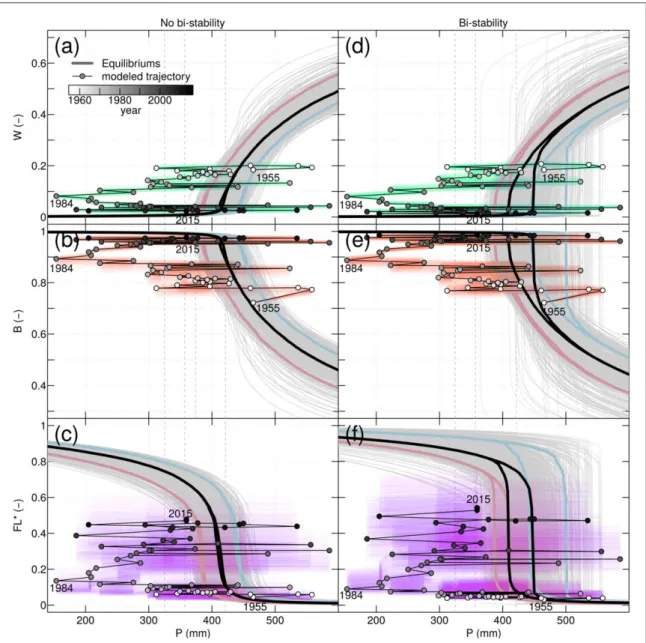
For all members, the system equilibrates to a degraded state(low W, high B and FL*) for P<350 mm, and to

Figure 1. Time series of simulated woody vegetation fraction W, bare soil fraction B and hydrological connectivity FL*for the ensemble of 1000 best simulations; black solid line: member with the lowest RMSE; dark blue line: observed rainfall; and circles: observed W and B fractions.

5

a vegetated state for P>580 mm (figure 2). The

fraction of woody cover W at equilibrium increases with the rainfall amount, and B and FL* decrease accordingly. The herbaceous cover fraction H at equilibrium(not shown) is about 0 for the degraded state and ranges from 0.03 to 0.1 for the vegetated one.

For 37% of the members, a single equilibrium state exists(monostability) for each rainfall amount, and the equilibrium value gradually changes with precipitation (figures2(a)–(c)). For the remaining members (63%),

the system is bistable over a range of P values where two equilibria coexist(figures2(d)–(f)). The bounds of the

bistability range correspond to the critical thresholds (tipping points) of the system, which delimit the range of P where the equilibrium state differs depending on whether the system is declining or regreening. The equilibrium curves(figure2) and the precipitation

cri-tical thresholds for mono- and bi-stable members (table3) are similar along the decline branches, but very

different along the regreening ones. Since observations were only available along the decline trajectory of the system, the regreening branches were poorly con-strained. Consequently, the value of the critical regreen-ing thresholds and the proportion of bistable members remain uncertain.

Figure 2. Equilibrium states of woody vegetation fraction W(a), (d), bare soil fraction B (b), (e), and flowlength FL*(c), (f) versus constant annual rainfall P, for ensemble members without(left column) and with bistability (right column). Quantiles 10, 50 and 90% of the distribution are emphasized(bold lines). For members with bistability (d)–(f), a decline and a regreening equilibrium coexist over a range of P. Vertical dotted lines represent the mean precipitation for each period of table1.

Table 3. Annual precipitation thresholds P_{(mm) for} quantiles 10, 50, and 90% of the ensemble members with and without bistability. For monostable cases, the rainfall threshold was defined as the value of P above which a runoff exists(R>0.1).

Quantile Monostability Bistability Decline Regreening

10% 387 390 412

50% 416 412 450

For all members, the degraded state was the only

one possible for drought (P = 325 mm) and

post-drought(P = 357 mm) mean precipitation (figure2).

For the pre-drought mean precipitation(P = 421 mm), an equilibrium vegetated state with low runoff exists for 73% of the members, of which an alternative degraded equilibrium exists for about one half of them. For the remaining 27%, the attracting equilibrium is the degra-ded one. All these results were obtained from an ensem-ble of parameter sets selected without taking into account the uncertainties on the observations, which we could not quantify(section2.3). We have shown

with a sensitivity analysis(supplementary section S8) that accounting for these uncertainties moderately changes the values of the critical thresholds and the pro-portion of mono- and bi-stable members. Nevertheless, the uncertainties do not affect the qualitative behavior described above and do not call into question the

existence of the two alternative stable states, nor the other conclusions of the study.

For most of the members, the system equilibrium is the vegetated/low runoff state before the drought, and the alternative low vegetation/high runoff state since then. However, equilibrium states do not provide infor-mation on actual trajectories because the way in which the system converges to these states depends on its evol-ution rate and on the rainfall variability.

3.3. Actual trajectories

When the model was initialized with the 1955 state and forced with the observed rainfall, all the simula-tions crossed several times the equilibrium curves during the pre-drought period, oscillating around a

vegetated state with W≈0.15, B≈0.80 and

FL*≈0.40 (figure 3). Due to a few very dry years

(around 1984) in the drought period, it was pulled far

Figure 3. Simulated trajectories for woody vegetation fraction W_{(a), (d), bare soil fraction B (b), (e), and flow length FL}*_{(c), (f)} obtained with observed annual rainfall from 1955 to 2015, for members without(left column) and with (right column) bistability, superimposed on the equilibrium curves offigure2. For each variable, the trajectory of the median member is emphasized(solid line with dots). The dot color varies with time (color scale), and dots corresponding to the beginning (1955), the drought peak (1984) and the end(2015) of the simulation period are labelled.

7

away from this equilibrium (to the left of the equilibrium curve), while W (resp. B, FL*_{) was} decreasing (resp. increasing). After the drought, the system remained in a degraded state, despite the occurrence of some wet years(P>450 mm) corresp-onding to a vegetated equilibrium. Although the range of rainfall variability in every subperiod encompassed P values associated with vegetated and degraded equilibrium, the system did not adjust to them (figure3), which means that its adjustment timescale is

larger than the timescale of rainfall variability.

These results suggest that the drop in the mean annual rainfall between 1970 and 1994 was a major driver of the observed decline of the Ortonde tiger bush. However, the inter-annual variability of rainfall may also have contributed to the destabilization of the system.

3.4. Sensitivity to rainfall variability

Except if the system is extremely slow(insensitive to forcing variability) or extremely reactive (it adjusts immediately to the equilibrium state corresponding to the forcing), the variability of the forcing and its temporal structure can drive oscillations of the system between states(Bathiany et al2018) and trigger critical

transitions(van der Bolt et al2018). The sensitivity of

the system to rainfall variability was assessed using synthetic annual rainfall series with prescribed mean,

standard deviation and lag-1 autocorrelation

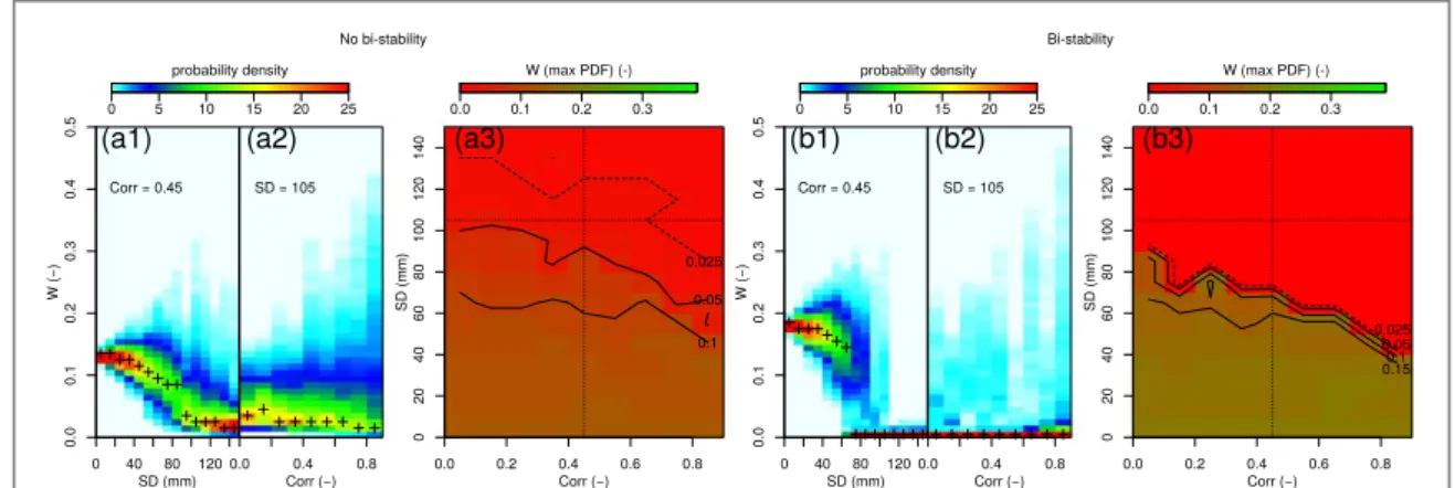
(section2.4). This sensitivity is illustrated in figure4

for the two members corresponding to the median

member (supplementary section S6) of the

mono-stable and the bimono-stable simulation subsets, initialized with the 1955 condition.

In the monostable case (figures 4(a1)–(a3)), the

distribution of W widens(blue colors) and the mode (most frequent value, crosses) decreases when SD

(figure4(a1)) and Corr (figure4(a2)) increase: the

sys-tem gradually shifts from a vegetated to a degraded state when the rainfall variability increases and/or when its temporal structure strengthens(figure4(a3)).

The increased dispersion of W for high values of SD and Corr means that the system can reach a high vege-tation states at some time, but it is attracted back to a low W state.

In the bistable case(figures4(b1)–(b3)), the same

type of behaviour is obtained except that beyond a SD

threshold (SD≈50 mm for Corr=0.45 in

figure4(b1)), the distribution of W becomes bimodal

(W≈0.15 and W≈0.01). For SD>80 mm, the dis-tribution abruptly shrinks and the mode shifts towards W≈0 (figure4(b1)). The shift to the

degra-ded state occurs for a lower variability(SD) when Corr increases(figure4(b3)). It means that due to longer

dry and wet periods(high Corr), less deviation from the mean rainfall is required to attract the system towards the degraded state(van der Bolt et al2018). In

all cases, the system forced with variable precipitation oscillates around a W(resp. B and FL*) value which is lower(resp. higher) than the equilibrium reached with a constant rainfall (SD=0 on figures 4(a1), (b1)).

Increased autocorrelation, which implies longer dry and wet periods, moves the system further from equi-librium during precipitation anomaly periods, which amplifies the effect of the inter-annual variability (figures4(a3) and4(b3)). This result can be interpreted

by asymmetric declining versus regreening processes: the system degrades more during dry years than it recovers during wet years, which pushes it to a more degraded state when rainfall variability increases.

These results confirm that no vegetated state was possible in both drought and post-drought periods, and that the system remained trapped in the basin of attraction of the degraded state until now. They also show that the reduction of the mean annual rainfall

Figure 4. Probability density of woody vegetation fraction W as a function of annual precipitation standard deviation SD and auto-correlation Corr for models initialized with the 1955 conditions and forced by 2000-year synthetic rainfall series with mean P_{=425 mm. Results for the median member of the ensemble without (a) and with (b) bistability. Probability density of W simulated} over the last 1000 years(see methods) as a function of SD for Corr=0.45 (a1), (b1) and of Corr for SD=105 mm (a2), (b2). SD_{=105 mm and Corr=0.45 were retrieved from the observed rainfall dataset. The crosses in a1, a2, b1, and b2 refer to the} maximal probability density of W(mode, the most frequent simulated state). Surface and contour lines of the mode of W in the SD versus Corr space(a3), (b3); the horizontal and vertical dotted lines a3 and b3 locate the observed values SD=105 mm and Corr=0.45.

during the drought period is sufficient to explain the observed decline of this tiger bush.

3.5. System resilience

With climate change, the inter-annual variability as well as the length of dry and wet periods may increase in central Sahel in the next decades (Monerie et al

2017, Martin 2018). In this region, there is no

consensus on the sign of annual precipitation change between global circulation models(Christensen et al

2014). Recent studies over the region showed that the

annual rainfall may increase in central Sahel(Giannini et al 2013, Park et al 2016, Monerie et al 2017),

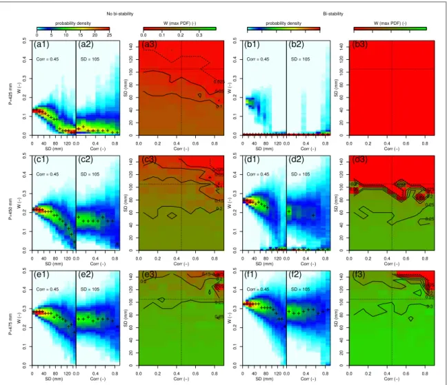
although this scenario is still uncertain. This trend could bring favourable conditions for the recovery of the Ortonde tiger bush. The resilience of the system, defined as its potential to recover a vegetated state with low runoff, was assessed with the same kind of analysis than in the previous section. The model was initialized with the current state(2014), and forced with synthetic rainfall series with increasing mean rainfall: P=425 mm (≈pre-drought), P=450 mm (+6%), and P=475 mm (+12%), and varying SD and Corr.

For the median monostable member, the system response to variable rainfall with pre-drought proper-ties is similar to that obtained with the 1955 initial conditions(figures5(a) and4(a)), and the current state

is stable(W≈0.025). For higher annual precipitation (figures5(c), (e)), the system recovers to W values that

are larger if P is large, except if both SD and Corr are high(figures5(c3) and (e3)).

For the median bistable member, the system remains on the degraded state for pre-drought mean precipitation, with little fluctuations (figure 5(b)),

whereas a vegetated state exists with the 1955 initial condition(figure4(b)). This difference underlines the

effect of the bi-stability: with the 2014 initial condi-tion, the system lies in the basin of attraction of the degraded state, whereas it is attracted by the alternative vegetated state with the 1955 condition. For P=450 mm, the system is bi-stable for 50 mm<SD<130 mm (Corr=0.45). Bi-stability almost disappears for P=475 mm, and the system recovers except when SD…110 mm and Corr…0.5 (figure 5(f)). Along with vegetation recovery, the

model simulates a reduction of the runoff capacity (supplementary section S7), associated with the reduc-tion of bare soil areas. However, the rills and gullies

Figure 5. Same asfigure4for mean annual rainfall P=425 mm (a), (b), P=450 mm (c), (d) and P=500 mm (e), (f), and initialization with the 2014 observed state. The dotted contour line(W=0.025) in (a3)–(f3) corresponds to the initial 2014 condition.

9

that developed on the site will hardly disappear. These durable physical changes imply that the system cannot recover following the same pathway back. As such changes in the hydrological structure are not repre-sented in our model, our results could overestimate the resilience of the system.

For all members the shift between states occurs for higher mean precipitation when the rainfall variability (SD and/or Corr) increases, e.g. the iso-value W=0.05 moves to domains with higher SD and Corr when P increases(figures5(a3)–(c3)–(e3), and (d3)–

(f3)). It implies that under variable precipitation for-cing, the regime shift will occur for higher precipita-tion values than assessed from constant rainfall (table3andfigure2).

According to the model, a regreening of the system from its current state is possible. It requires the mean annual precipitation to be at least equal to its pre-drought value(P≈425 mm) which is sufficient if the rainfall variability is low and if the system is not bis-table. If the system is bistable, a higher mean precipita-tion is required, at least equal to the regreening critical threshold for constant rainfall(figure2and table3).

This value is not sufficient considering annual rainfall variability, as illustrated infigure5(d3) for the median,

bistable member: with the current rainfall variability (SD=105 mm, Corr=0.45), P=450 mm is no longer sufficient for regreening, whereas it is the regre-ening threshold in table3.

Considering the future rainfall increase as a work-ing assumption, we have estimated from Monerie et al (2017) that the mean annual precipitation may reach

about 475 mm by the end of the 21st century in North-ern Mali. Similarly, the rainfall variability may increase, with an estimated SD increment of about 50 mm. Thus, according to our simulations, the simultaneous increase in annual totals and inter-annual rainfall variability would lead to antagonistic effects on the resilience of the system and, therefore, an uncertain future. The red noise model used to assess the effect of rainfall variability poorly represents the strong decadal structure of Sahelian rainfall (Dieppois et al2013), and the effect of the temporal

structure of rainfall may be stronger than estimated. Furthermore, a larger intraseasonal variability is also anticipated in a warmer climate(Martin2018), which

could also affect the potential for resilience.

In addition to the intraseasonal rainfall variability and the hydrological effects of rills, other factors such as air temperature have been omitted in our simple model. We used rainfall as unique forcing because vegetation and runoff changes were more driven by rainfall than temperature changes over the past dec-ades(Hiernaux et al2009,2009, Leauthaud et al2017).

Temperature increase is a robust trend globally (Christensen et al2014), it and could play a major

eco-hydrological role in the future. Increased temper-ature-controlled evaporation may increase the water

stress(Young et al2017). However the effects of higher

temperature on the physiology of tropical plants are largely unknown and deserve specific studies (Jones1992, Cavaleri et al2015). Although direct and

indirect temperature effects are uncertain, it is prob-able that higher temperature will reduce rather than improve the future resilience of Sahelian ecosystems.

4. Conclusions and prospects

We developed a system dynamics model to represent the ecohydrological evolution of a Sahelian tiger bush over decades, constrained by observation data. The model represents thefirst order interactions (includ-ing retroactions) between hydrology and vegetation. Although based on a simple representation of the studied tiger bush, the model was able to reproduce the observed vegetation decline and the associated increase in surface runoff over the 1955–2015 period. Based onfield work, these trends are robust and are iconic of the declining systems in the region. Accord-ing to our simulations, the system was oscillatAccord-ing around a vegetated state before the 1970–94 drought, as a response to rainfall variability. Then it started to shift to a degraded(low vegetation/high runoff) state around which it currently remains, despite a slight rainfall recovery. We have confirmed that this decline corresponds to a shift between two stable states: a vegetated/low runoff state and a low vegetation/high runoff state. The drop in the mean annual precipita-tion associated with the drought was found to be sufficient to explain this regime shift. We could not conclude whether the shift occurred as a gradual response to the changing forcing or if it implied critical transitions (hence bistability), both modalities of change being plausible in our simulation ensemble.

We showed that increased variability in annual rainfall(amplitude of variation and temporal struc-ture) pushes the system towards more degraded states. Rainfall increase in central Sahel is a possible trend anticipated in some climate change scenarios, but its effect on vegetation recovery may be offset by the con-current increase expected in rainfall variability. According to our simulations, the Sahelian tiger bush is resilient. However, as the model was only con-strained along the decline trajectory observed on a particular site, the critical rainfall conditions for resi-lience could not be evaluated precisely. Moreover, the simple model structure and some unaccounted pro-cesses(impacts of higher temperature, effect of gullies) might well lead to over-estimate the resilience of the system. Our study has yielded robust qualitative con-clusions on the existence of alternative stable states in such systems and on their resilience potential, but due to the remaining uncertainties we could not make quantitative predictions.

The main conclusion of this study is that a drought-induced regime shift can explain the runoff increase observed at the hillslope-scale in some Sahe-lien landscapes. In a future work, the model will be applied to various sites representative of the diversity of Sahelian ecohydrosystems, including regreening ones(Dardel et al2014). This will quantify the role of

hillslope-scale regime shifts in the concurrent regreen-ing and runoff increase trends observed at the regional scale.

Acknowledgments

This study was funded by IRD through a post-doctoral fellowship contract. It has been realized with the support of the High Performance Computing Platform

MESO@LR, financed by the

Occitanie/Pyrénées-Méditerranée Region, Montpellier Mediterranean Metropole and the University of Montpellier(France). The authors are grateful to the Malian Meteorological Service for the historical rainfall datasets. Recent observations were provided by the AMMA-CATCH observatorywww.amma-catch.org. The authors thank V Dakos and S Kéfi for fruitful discussions about this work, and the two anonymous reviewers for their input, which improved the manuscript.

Data availability statements

The data that support thefindings of this study are presented in Trichon et al (2018). The land cover

dataset, derived from Trichon et al(2018), is given in

supplementary section S1(table S1). The yearly rainfall series at the Hombori meteorological station, from the Malian Meteorological Service and the AMMA-CATCH Observatory(Galle et al2018), is not publicly

available for legal reasons, but it is available from the corresponding author upon reasonable request.

ORCID iDs

Valentin Wendling

https://orcid.org/0000-0003-4163-9700

Christophe Peugeot

https://orcid.org/0000-0003-2161-125X

Angeles G Mayor https: //orcid.org/0000-0001-8097-5315

Pierre Hiernaux

https://orcid.org/0000-0002-1764-9178

Eric Mougin https: //orcid.org/0000-0002-7569-5906

Manuela Grippa https: //orcid.org/0000-0002-4889-7975

Laurent Kergoat

https://orcid.org/0000-0003-1792-8473

Romain Walcker https: //orcid.org/0000-0002-5769-810X

Sylvie Galle https: //orcid.org/0000-0002-3100-8510

Thierry Lebel

https://orcid.org/0000-0002-1297-6751

References

Barnosky A D et al 2012 Nature486 52–8

Bathiany S, Scheffer M, Nes E H V, Williamson M S and Lenton T M 2018 Sci. Rep.8 5040

Broderstad E G and Eythorsson E 2014 Ecol. Soc.19 1

Brook B W, Ellis E C, Perring M P, Mackay A W and Blomqvist L 2013 Trends Ecol. Evol.28 396–401

Casenave A and Valentin C 1992 J. Hydrol.130 231–49 Cavaleri M A, Reed S C, Smith W K and Wood T E 2015 Global

Change Biol.21 2111–21

Christensen J et al 2014 2013: Climate phenomena and their relevance for future regional climate change Climate Change 2013: The Physical Science Basis. Contribution of Working Group I to the Fifth Assessment Report of the Intergovernmental Panel on Climate Change ed T F Stocker et al(Cambridge: Cambridge University Press) pp 1217–308

Claussen M, Kubatzki C, Brovkin V, Ganopolski A,

Hoelzmann P and Pachur H J 1999 Geophys. Res. Lett.26 2037–40

Cueto-Felgueroso L, Dentz M and Juanes R 2015 Phys. Rev. E91 052148

Dardel C, Kergoat L, Hiernaux P, Grippa M, Mougin E, Ciais P and Nguyen C C 2014 Remote Sensing6 3446–74

Dardel C, Kergoat L, Hiernaux P, Mougin E, Grippa M and Tucker C 2014 Remote Sens. Environ.140 350–64

Deblauwe V, Barbier N, Couteron P, Lejeune O and Bogaert J 2008 Global Ecol. Biogeogr.17 715–23

Descroix L, Genthon P, Amogu O, Rajot J L, Sighomnou D and Vauclin M 2012 Global Planet. Change98-99 18_–30 Descroix L et al 2018 Water10 748

d’Herbés J M, Valentin C, Tongway D J and Leprun J C 2001 Banded Vegetation Patterning in Arid and Semiarid Environments: Ecological Processes and Consequences for Management ed D J Tongway, C Valentin and J Seghieri(New York: Ecological Studies Springer) pp 1–19

Di Baldassarre G, Viglione A, Carr G, Kuil L, Salinas J L and Blöschl G 2013 Hydrol. Earth Syst. Sci.17 3295–303 Dieppois B, Diedhiou A, Durand A, Fournier M, Massei N, Sebag D,

Xue Y and Fontaine B 2013 J. Geophys. Res.: Atmos.118 12587–99

D’Odorico P, Bhattachan A, Davis K F, Ravi S and Runyan C W 2013 Adv. Water Res.51 326–44

Downey S S, Haas W R and Shennan S J 2016 Proc. Natl Acad. Sci. 113 9751–6

Favreau G, Cappelaere B, Massuel S, Leblanc M, Boucher M, Boulain N and Leduc C 2009 Water Resour. Res.45 W00A16 Fensholt R et al 2012 Remote Sens. Environ.121 144_–58

Gal L, Grippa M, Hiernaux P, Peugeot C, Mougin E and Kergoat L 2016 J. Hydrol.540 1176–88

Gal L, Grippa M, Hiernaux P, Pons L and Kergoat L 2017 Hydrol. Earth Syst. Sci.21 4591–613

Galle S, Ehrmann M and Peugeot C 1999 CATENA37 197–216 Galle S et al 2018 Vadose Zone J.17 180062

Gardelle J, Hiernaux P, Kergoat L and Grippa M 2010 Hydrol. Earth Syst. Sci.14 309–24

Giannini A, Salack S, Lodoun T, Ali A, Gaye A T and Ndiaye O 2013 Environ. Res. Lett.8 024010

Gollini I, Pianosi F, Sarrazin F and Wagener T 2015 SAFER: Sensitivity Analysis For Everybody with R. R package version 1.1(http://bristol.ac.uk/cabot/resources/safe-toolbox/) Heino M, Ripa J and Kaitala V 2000 Ecography23 177–84 Hiernaux P, Ayantunde A, Kalilou A, Mougin E, Gérard B, Baup F,

Grippa M and Djaby B 2009 J. Hydrol.375 65–77 Hiernaux P, Diarra L, Trichon V, Mougin E, Soumaguel N and

Baup F 2009 J. Hydrol.375 103_–13

11

Hiernaux P and Gérard B 1999 Acta Oecologica20 147_–58 Hiernaux P, Mougin E, Diarra L, Soumaguel N, Lavenu F, Tracol Y and Diawara M 2009 J. Hydrol.375 114–27 Hirota M, Holmgren M, Nes E H V and Scheffer M 2011 Science334

232–5

Holmgren M, Hirota M, van Nes E H and Scheffer M 2013 Nat. Clim. Change3 755–8

Hughes T P, Carpenter S, Rockström J, Scheffer M and Walker B 2013 Trends Ecol. Evol.28 389–95

Hughes T P, Linares C, Dakos V, van de Leemput I A and van Nes E H 2013 Trends Ecol. Evol.28 149–55

Jones H G 1992 Plants and Microclimate: A Quantitative Approach to Environmental Plant Physiology(Cambridge: Cambridge University Press)

Kefi S, Eppinga M B, de Ruiter P C and Rietkerk M 2010 Theor. Ecol. 3 257–69

Kefi S, Holmgren M and Scheffer M 2016 Funct. Ecol.30 88–97 King E G, Franz T E and Caylor K K 2012 Ecohydrol.5 733–45 Kuil L, Carr G, Viglione A, Prskawetz A and Blöschl G 2016 Water

Resour. Res.52 6222_–42

Le Barbe L, Lebel T and Tapsoba D 2002 J. Clim.15 187–202 Leauthaud C et al 2017 Int. J. Climatol.37 2699–718 Lebel T and Ali A 2009 J. Hydrol.375 52–64 Lenton T M, Held H, Kriegler E, Hall J W, Lucht W,

Rahmstorf S and Schellnhuber H J 2008 PNAS105 1786–93 Ludwig J A and Tongway D J 1995 Landscape Ecology10 51–63 Mahé G and Paturel J E 2009 C.R. Geosci.341 538–46 Martin E R 2018 Geophys. Res. Lett.45 11913–20

Mayor A G, Bautista S, Small E E, Dixon M and Bellot J 2008 Water Resour. Res.44 W10423

Mayor A G, Kéfi S, Bautista S, Rodríguez F, Cartení F and Rietkerk M 2013 Landscape Ecology28 931–42

Monerie P A, Sanchez-Gomez E, Pohl B, Robson J and Dong B 2017 Environ. Res. Lett.12 114003

Okin G S, Heras M M D L, Saco P M, Throop H L, Vivoni E R, Parsons A J, Wainwright J and Peters D P 2015 Frontiers in Ecology and the Environment13 20_–7

Panthou G, Lebel T, Vischel T, Quantin G, Sane Y, Ba A, Ndiaye O, Diongue-Niang A and Diopkane M 2018 Environ. Res. Lett. 13 064013

Park J Y, Bader J and Matei D 2016 Nature Clim. Change6 941–5 Peugeot C, Esteves M, Galle S, Rajot J L and Vandervaere J P 1997

J. Hydrol.188-189 179–202

Pianosi F, Sarrazin F and Wagener T 2015 Environ. Modelling Softw. 70 80–5

R Core Team 2018 R: A Language and Environment for Statistical Computing(Austria: R Foundation for Statistical Computing Vienna)

Rietkerk M, Dekker S C, Ruiter P C D and Koppel J V D 2004 Science 305 1926_–9

Rodríguez F, Mayor A G, Rietkerk M and Bautista S 2018 Ecol. Indic. 94 512–9

Ruokolainen L, Lindén A, Kaitala V and Fowler M S 2009 Trends Ecol. Evol.24 555–63

Saco P M, Moreno-de las Heras M, Keesstra S, Baartman J, Yetemen O and Rodríguez J F 2018 Current Opinion in Environmental Science & Health5 67–72

Saco P M, Willgoose G R and Hancock G R 2007 Hydrol. Earth Syst. Sci.11 1717–30

Scheffer M 2009 Critical Transitions in Nature and Society (Princeton, NJ: Princeton University Press)

Scheffer M, Carpenter S, Foley J A, Folke C and Walker B 2001 Nature413 591

Scheffer M and Carpenter S R 2003 Trends Ecol. Evol.18 648–56 Sivapalan M 2015 Water Resour. Res.51 4795–805

Soetaert K, Petzoldt T and Setzer R W 2010 J. Stat. Software33 1–25 Staver A C, Archibald S and Levin S 2011 Ecology92 1063_–72 Steffen W et al 2018 Proc. Natl Acad. Sci.115 8252_–9

Tamagnone P, Massazza G, Pezzoli A and Rosso M 2019 Water11 156 Taylor C M, Belušić D, Guichard F, Parker D J, Vischel T, Bock O,

Harris P P, Janicot S, Klein C and Panthou G 2017 Nature544 475–8

Trichon V, Hiernaux P, Walcker R and Mougin E 2018 Global Change Biol.24 2633–48

Turnbull L, Wainwright J and Brazier R E 2008 Ecohydrology1 23–34

UN 2017 World population prospects. the 2017 revision. key findings and advance tables Technical Report ESA/P/WP/ 248 United Nations, Department of Economic and Social Affairs, Population division

Valentin C, d’Herbès J M and Poesen J 1999 CATENA37 1–24 van der Bolt B, van Nes E H, Bathiany S, Vollebregt M E and

Scheffer M 2018 Nat. Clim. Change8 478–84

van Nes E H, Hirota M, Holmgren M and Scheffer M 2014 Global Change Biol.20 1016_–21

Vetter S 2005 J. Arid. Environ.62 321_–41

Wilcox B P, Le Maitre D, Jobbagy E, Wang L and Breshears D D 2017 Rangeland Systems: Processes, Management and Challenges ed D D Briske(Cham: Springer)pp 85–129 Wilcox C, Vischel T, Panthou G, Bodian A, Blanchet J, Descroix L,

Quantin G, Cassé C, Tanimoun B and Kone S 2018 J. Hydrol. 566 531–45

Yin Z, Dekker S C, van den Hurk B J J M and Dijkstra H A 2014 Earth Sys. Dyn.5 257–70

Young D J N, Stevens J T, Earles J M, Moore J, Ellis A, Jirka A L and Latimer A M 2017 Ecol. Lett.20 78–86