*-- --- -.- --- iT~'
~
~b
~
~
~ ~
_~~180 WATER: THERMAL AND DYNAMICAL BALANCES. by
JOHN LEE LILLIBRIDGE III B.S., University of Washington
(1976)
SUBMITTED IN PARTIAL FULFILLMENT OF THE REQUIREMENTS FOR THE
DEGREE OF .SCIENCE MASTER'S
at the
MASSACHUSETTS INSTITUTE OF TECHNOLOGY SEPTEMBER 1979
Signature of Author... 1/.... ....E~Y. . r...
J
Department of Meteorolo , September 7, 1979Certified by... . v.<.7 .V . r... . ... -- - c... Dr. Mic S. McCartney
Accepted by ...-... ... ...
Chairman, Department Committee
180 WATER: THERMAL AND DYNAMICAL BALANCES by
JOHN LEE LILLIBRIDGE III
Submitted to the Department of Meteorology
on September 7, 1979 in partial fulfillment of the requirements for the Degree of Science Master's
ABSTRACT
A simple ocean model applicable to the return flow region of the North Atlantic subtropical gyre is formulated to assess the dynamical effects of surface heat fluxes. The model is based on the thermodynamical model developed by Warren (1972). Warren's model satisfies the vertically integrated heat equation of the seasonal layer by means of a vertical temperature prescription which depends only on the surface temperature. The surface heat fluxes in his model also depend on the sea temperature, so that the model can adjust itself to a state in which heat storage changes in the seasonal layer balance the surface heat fluxes. A scale analysis indicates that Warren's model is applicable even for our full ocean depth, extended model.
The thermodynamics force the dynamics in this model by changing the pressure field of the seasonally influenced layers. The model has two free unknowns, the free surface and main thermocline positions, which are governed by two vertically integrated, quasigeostrophic vorticity equations.
The model results indicate that the main response of the free sur-face is due to thermal expansion. The nonisostatic response gives rise to transports over 1000 km of less than 5 Sverdrups. The main thermocline response is only a few meters when subjected to small scale forcing,
and has a much smaller response to the observed large scale forcing. Larger changes in the circulation resulted during deep convection and eighteen degree water formation, because of larger potential energy changes associated with the buoyancy fluxes in late winter. Even so, only small transport changes across the gyre were indicated. It is con-cluded that the model response was much weaker than that observed, and that the consideration of wind effects would probably be necessary to better model the observed seasonal and year to year variability within the eighteen degree water formation region.
Thesis Supervisor: Dr. Michael S. McCartney
Title: Associate Scientist, Department of Physical Oceanography, Woods Hole Oceanographic Institution.
Table of Contents Page Abstract 2 I. Introduction 5 A. Observations 5 B. Warren Model 7 II. Theory/Scaling 13 A. Introduction 13 B. Thermodynamic Equation 15 C. Mass/Continuity 26 D. Dynamics 28
III. Solution of Equations/Numerical Method 41
A. Form of Forcing and Boundary Conditions 41
B. Method of Solution 45
C. Analytic Nature of Equations 51
IV. Numerical Model Results/Discussion 56
A. Introduction 56
B. End of Heating Results 58
C. End of Convection Results 67
V. Conclusions 72 References 80 Acknowledgments 81 Figure Captions 82 Figures 85 Table Captions 104 Tables 105
Appendix A - Dynamical Scale Analysis 110
Appendix B - Double Integral Trapezoidal Approximation 117
I. Introduction
A. Observations
Many models of the large scale, wind-driven ocean circulation have been formulated, and these have been largely successful in mimicking ob-served features in the ocean. Thermohaline processes have also received some attention, but models of this type of dynamic forcing have concen-trated largely on deep abyssal flows driven by mass sources and sinks.
On the other hand, there is an abundance of surface mixed layer models which focus on the role of buoyancy fluxes and wind stirring in the creation and destruction of the near surface seasonal thermocline. These models often use energetic closure arguments, but generally do not study the dynamics forced by the presence or absence of the seasonal thermocline; they are inherently small scale, local models.
Worthington (1972b) drew attention to the possible importance of thermal forcing to the large scale circulation in the subtropical gyres. He has also proposed (Worthington,(1976))that the seasonal heating cycle may be responsible for fluctuations in the circulation around the sub-tropical gyres. He suggests that the formation in late winter of deep isothermal mixed layers south of the western boundary currents may in-crease the transport of the anticyclonic gyre. For example, Worthing-ton attributes the observed variability in Gulf Stream transport to deepening of the main thermocline in late winter associated with the formation of "Eighteen Degree Water." This formation process is due to seasonally large negative heat fluxes from the ocean which cause deep vertical convection and mixing. The data basis for the temporal
transport variability originated as Figure 44 of Worthington (1976). An updated compilation of Gulf Stream transports (0 relative to
2000 db) from the "Bermuda triangle" (Montauk-Bermuda-Hatteras) is presented in Figure 1. It can be seen from this that there is some
evidence of seasonal variability, but that year to year variations for any month can be as large as the amplitude of the seasonal signal 1"10-30 Sverdrups. This long-term variability is attributed
(Worthington, (1972b)) to "severe" winters in which there are outbreaks
of extremely cold, polar continental air and associated anomalously large negative heat fluxes. Worthington believes that there is a deep-ening of the underlying main thermocline associated with production of excessive amounts of Eighteen Degree Water in these severe winters. As a possible mechanism for the main thermocline deepening, Worthington
(1972b), Figure 4 suggests a meridional circulation scheme. In this schematic figure he proposes that during severe winters, and excessive Eighteen Degree Water formation, there is an associated convergence of
near surface waters from the south into the "formation" region south of the Gulf Stream. These warm waters are rapidly cooled to the am-bient surface temperature and mixed into the homogeneous layer. Some of this excess convergence, or the downward motion of the water itself,
is envisioned as causing the main thermocline to be forced downward. The meridional cell is closed by the southward extension of Eighteen Degree Water, flowing above the main thermocline but below the near
surface waters which are moving northwards. Worthington suggests that at least part of the mean anticyclonic circulation in the Sargasso Sea
These comments are illustrated in Figure 2 by a pair of hydro-graphic stations taken in the Eighteen Degree Water formation region in a relatively mild and a severe winter. The increased depth of the homogeneous layer in the Researcher station cannot be due solely to convective erosion'into the main thermocline, since the temperature is still nearly 180. Erosion into the roughly 50 m/*C gradient of the main thermocline would be associated with a several degree temperature drop, if mixing alone was the cause of this 100-200 m deepening. Thus the question is whether this main thermocline heaving, and associated baroclinic transport changes, are- being driven by the thermodynamic forcing, whether it is associated with changes in the wind-driven circulation in the subtropical gyre as a whole, or possibly if it is driven by the local Ekman pumping. It is the intent of this study to investigate the first possibility.
B. Warren Model
Warren (1972) formulated a seasonal thermocline model applicable to the local heat balance in the formation region of Eighteen Degree Water. In his model a linearized and continuous vertical temperature
structure is specified at a point in the formation region. The profile has specified seasonal and main thermocline gradients, with the depth of the main thermocline fixed. With this prescription the structure is only dependent on the surface temperature. However, this dependence changes depending on whether the water column is building a seasonal
and eroding into the main thermocline. Thus, the way in which the heat content of the column changes at any point depends upon the phase of the heating cycle to which a column of fluid is being subjected. His vertical temperature profile was modeled after the observed temperature field and an example he used for the North Atlantic is shown in Figure 3.
Since the model is envisaged for the central formation region of Eighteen Degree Water, where both zonal and meridional gradients
locally go to zero, Warren can neglect horizontal advection and diffu-sion immediately. He also assumes the surface heat flux is much
greater than vertical diffusion or advection into or out of the seasonal thermocline. These surface heat fluxes depend on sea surface tempera-ture so that the forcing has feedback from the ocean. The effect of the heat flux on the atmosphere is neglected, so that the atmospheric variables are assumed given by observations. He arrives at a purely local model in which heat storage, a function of surface temperature as well as the history of surface temperature, balances the atmospher-ically forced surface heat fluxes, which also depend on surface
temperature.
In his model, Warren integrates the heat equation forward in time from an initial state of excessive heat content, relative to the imposed atmospheric state. This forces a net heat loss for several years and consequently leads to late winter deep convection during those years. He finds that the seasonal limit cycle into which the surface tempera-tures settle is very close to that observed, if observed atmospheric forcing were used. In this limit cycle, the surface temperature and
therefore the heat fluxes have adjusted to a state where no late winter convection, and no net annual heat loss, occurs. When this limit
cycle was subjected to a "severe" winter he found that although ero-sion into the main thermocline occurred, it was minimized because the seasonal thermocline had to be eroded away first, and then the homo-geneous layer below was of such large vertical extent that a very large heat loss was required to change the surface temperature significantly.
Warren's model is a simplified solution to the depth integrated heat equation for the upper waters which are influenced by seasonal heat fluxes. The associated buoyancy fluxes and the dynamical response they excite are not, however, addressed. The model vertical structure
in his formulation does not have the freedom to satisfy the depth integrated dynamical equations.
In an attempt to model the dynamical consequences of the seasonal heating cycle and Eighteen Degree Water formation, we decided to build upon the successful thermodynamic framework that Warren's model
employed. We extend his model by giving the vertical prescription more degrees of freedom, so that it has dynamical response, and then
reconstrain the system with depth integrated dynamic equations.
We first removed the constraint of the "pinned" main thermocline by no longer requiring a fixed temperature at a fixed main thermo-cline depth. We don't intend that the temperature within the main thermocline should be changed by the surface heating, but rather that the main thermocline is. bodily heaving and vertical advection would thereby give rise to a change in temperature at a fixed depth. This
heaving would be associated with concommitant divergences or conver-gences within the overlying Eighteen Degree Water and seasonal layers and within the underlying deep layers. The vertical temperature prescription is extended to full ocean depth, but to rule out topo-graphic effects we consider a constant depth ocean. In order for the temperature structure to reamin realistic we prescribe a main thermo-cline of finite thickness with an underlying deep layer. Again for
simplicity, the deep waters are considered to be of uniform temperature
both vertically and horizontally. This prescription is illustrated in Figure 4.
We also make the kinematical prescription that the bottom of the thermocline is a material, as well as isopycnal, surface, and specify no flow through it. The interface at the bottom of the Eighteen Degree Water layer is not at constant temperature and is eroded during deep convection; thus it is not suitable as a material surface. We have given our model the freedom to respond like a two-layer model with the interior interface lying over a constant density bottom layer, but in our case the density varies continuously, rather than jumping, at that boundary. We make the simplification that when the main thermocline is not being eroded, its temperature gradient as well as thickness remain constant, though it may heave as a whole. This is, in part, based on observations, as can be seen in Figure 2, and is described further in Worthington (1972b)[cf. Figure 5 ]. With the main thermocline thick-ness constant, our material surface becomes the only internal, dy-namical unknown. We wish to allow for the possibility that the system
will respond in an external manner, and complete the "two-layer" analogy by allowing another variable, material interface at the free surface. We now have two dynamical unknowns in our model which will be constrained by two dynamical, in our case vorticity, equations.
It is necessary to extend the model horizontally as well as vertically to allow for gradients. Our region of interest lies in an area where the Gulf Stream and returning flow are primarily zonal, thus we only extend the model to 2-D and consider a meridional plane running along 550W with all quantities independent of the zonal
direc-tion. We will retain the local nature of Warren's thermodynamic model and will eventually integrate our dynamic equations in such a way as
to obtain a quasi-local form in these as well.
We envisage the thermodynamic forcing as entering the dynamics through its effect in changing the density of the seasonally influenced layer and thereby changing our prescribed density and pressure field hydrostatically. It will be shown in the next chapter that although the thermodynamics play a role in the dynamics, to first order it is justified to neglect the effect of the dynamics on the thermodynamics. This arises mainly because horizontal advection is small for this 2-D limit. With this oversimplification, we can take the thermodynamic ef-fects on the pressure field as given, with two free parameters,
governed by two vorticity equations, able to respond to this forcing. The form of the equations rendered will thereby be similar to the classical two-layer model of Veronis and Stommel (1956) but with a much different forcing from the buoyancy fluxes rather than the wind
In summary, the model we propose is primarily locally forced, as in Warren (1972), but focuses on the coupled internal/external dynamical response of the system to thermodynamic forcing (via hydro-statics and geostrophy). The forcing is taken as given, and not affected by the dynamic response which ensues. Because we have un-coupled the thermodynamics in this way, it is much simpler to specify the time and space variability of the heat fluxes, based on the obser-vations described by Bunker (1976) and Bunker and Worthington (1976), rather than specifying only the atmospheric fields and allowing the heat fluxes to adjust via the surface temperature. This is again an oversimplification since negative feedback will occur between the ocean and its thermal driving, but since we are trying to establish the nature of the dynamical response to the heat fluxes, we will be-gin with the fluxes taken as given by.Bunker's calculations.
It should be kept in mind that models of this type only satisfy certain integral conservation equations. Thus although the depth in-tegrated equations may be satisfied, one cannot expect that internally, the unintegrated equations will be exactly satisifed. The purpose of the imposed vertical temperature prescription is to mimic the internal response with a simplified, but nonetheless plausible, set of free variables.
We proceed in the next section to the theory necessary to derive our extended model equations.
II. Theory/Scaling
A. Introduction
Rather than developing a complete and systematic set of scaling arguments, in the following, only simple order of magnitude estimates of terms will be utilized to obtain a simplified system of conservation equations from the general equations. In making the magnitude estimates, our temperature prescription will be utilized whenever possible. This is done in part because the vertical prescription is a fair approxima-tion to the observed profile, and also because we will ultimately be utilizing this prescription in our model equations.
We make here a few a priori approximations and specifications. First, in computing vertical integrals of the density field we will assume exact hydrostatic balance, Secondly, we will completely neglect effects of horizontal diffusion of momentum and heat. Because of the absence of horizontal boundaries we expect that, in general, vertical diffusion of momentum will dominate horizontal momentum diffusion.
Similarly we expect vertical heat diffusion to dominate horizontal diffu-sion. Since our region of interest remains south of the Gulf Stream, horizontal mixing by eddies can presumably be neglected relative to vertical processes.
We will also neglect vertical diffusion of momentum in order to isolate the thermally-driven effects from the wind-driven field; we won't consider here the ultimate dissipation mechanism of the bottom boundary layer.
Thirdly, we make a rather strong specification on the vertical diffu-sion of heat or buoyancy. We will assume that below the layer of seasonal influence vertical diffusion of heat is very small, much smaller than the surface heating. We don't expect any internal buoyancy sources, and neglect the vertical diffusion which would tend to smooth regions of
rapid change in slope. Since we are specifying a profile with discontinu-ous slope, these diffusion effects would be large, but only in limited vertical regions. Since we are using the simplest vertical structure to obtain the essence of this system's response, the neglect of vertical
dif-fusion in slightly changing the shape seems justifiable.
Probably the most fundamental assumption we will be making is that there is a large asymmetry between the zonal and meridional length scales. Just how two dimensional the field must be to obtain a consistent set of equations will be discussed in a following section. The simplifications obtained in the 2-D limit will be quite far-reaching. One immediate
simplification that results will be the neglect of horizontal advection relative to time rate of change. In the following sections a Cartesian coordinate system is used even though our meridional scale is 1000 km. We neglect the metric terms from the full spherical equations in the
following discussion because they are generally the same order as advec-tion and would be neglected ultimately. One excepadvec-tion is a term in the continuity equation which is neglected assuming a priori that L tan
0/a
<< 1y
where L is the meridional scale, 8 is latitude and "a" is the earth's
y
We will combine the equations for heat and salt conservation to obtain a density equation, since density integrals will enter the
dynamical equations. This will be done using the simplest linear equa-tion of state. However, we will be focusing only on buoyancy fluxes associated with surface heat fluxes. This is not to say that mass and/or salt fluxes associated with differences between evaporation and precipita-tion are unimportant. We simply wish to focus on the effect of the
seasonal heating forcing.
Lastly, we will be using the Boussinesq approximation throughout to neglect the variations in density relative to a constant mean value, when density appears as a coefficient in the equations.
B. Thermodynamic Equation
Conservation of potential temperature and salt, with neglect of horizontal diffusion, can be written:
DO aQH
pc - = )
p Dt az
DS aQS
p
=
(2)
where
0
is potential temperature; S is salinity; QH and QS are vertical fluxes of heat and salt, respectively; p is in situ density; c isPspecific heat at constant pressure, treated here as a constant for sea-water of c = .93; and D/Dt is the substantial derivative following a
p
16
Our linear equation of state relating potential density to poten-tial temperature and salinity is:
Pe = Po ( - ,(-O0 ) + (S-So)) (3)
where po is a constant value of average density at temperature 0o and salinity So, and a,, 8, are the thermal and haline expansion coeffi-cients. We form a density equation from (1) and (2) by multiplying by
-poa, and po,*, respectively, and adding to yield:
Dp PaQ C,
Dt p zz p c QH + S (4)
By considering potential density we have included the first order effects of compressibility but we have neglected any second order effects between temperature, salinity, and pressure. The subscript 0 will now be dropped
though we will still be referring to the potential density. In deriving
equation (4) we have neglected variations in c, and
S,
relative to those ine
and S in the first term in (4). This is done in anticipation of the neglect of vertical diffusion below the seasonally influenced layer, since a, and6,
do change by about a factor of two be-tween the surface and deep waters, but we wish to neglect secondorder effects on p below this layer.
We now make scaling arguments to simplify our density equation. As in Warren's model, we shall consider the thermodynamic balance of a
vertical column of unit area. Therefore, in making our approximations we will explicitly use vertical integrals of our prescription to esti-mate orders of magnitude layer by layer,
Referring again to Figure 4, we see that without diffusion from the main thermocline our thick lower layer cannot change in time since there are no lateral or vertical density gradients specified. Of course there is a weak vertical gradient in the sub-thermocline waters, and generally non-negligible meridional gradients as well. Were we to in-clude these effects, the arguments for the density equation in the deep water would be similar to those that follow for the main thermocline.
Thus for the lower layer:
f -H -H - dz =- u Vp dz 0 (5) -B -B or S-B pdz = -pH (5a) at f-H at
Within the main thermocline, neglecting vertical diffusive effects at the boundaries, we have:
f
-D -D
- dz = - u V p dz (6)
-Ha -H
The density prescription is a mirror image of Figure 4, with the same subscript nomenclature on p, but with seas-onal and main thermocline gradients y and 6.
aH aD -D
z =
-H t- -D at -H
In our
constant in
prescription we assume the y as well as z so that the
main thermocline gradient,
8,
is advection term can be written as:-D u * Vp dz = 8 I-D -H -H 3H [w + v
ay
+ay
-D - 3H u * Vp dz= ${w+v + -H y -aH
u "} *(H-D)ax
where overbars -indicatevertical averages. Since we will be specifying
no cross-isopycnal flow at z = -H, the kinematic boundary condition there will be w = -[V + u -- + -]
-H -H y -H ax at
Since isopycnals are roughly parallel within the main thermocline, to a good approximation:
-- -7H -
aH
aH
w= -[v- + u
-+-ay
ax
at
Thus we find from (6a):
a
-D
aH
aD
aH
a- D dz = H a p " +
8
3 (H-D)at J-H at -D at at
Without deep convection aH/at = aD/at and we always have, by our pro-file, that p-D =-H + 8 (H-D). Substituting these above gives the ex-pected result:
a
-Dat I-H
u V p dz (6a) oraH
u -- ]dz ax--_ Ht pdz = 0 . (6b)
Thus, the mass of the main thermocline remains constant when not eroded.
If deep convection occurs, the main thermocline thickness (H-D) will
I
-Dbe changed proportional to the heat flux. In this case - pdz =
-H
P (H-D) Q. This will be discussed further when treating the seasonal layer.
In the homogeneous eighteen degree water layer there are no vertical advective or diffusive fluxes. We have specified that without deep con-vection the late winter density doesn't change, but we really mean it would only be altered slightly by horizontal advection. We show this as follows: In anticipating the 2-D limit of our momentum equations it can be shown that the meridional velocity, v, is of order (w/f) times the zonal velocity, u (w,f being the seasonal and inertial frequencies). In the 2-D limit, only meridional advection can be important, thus
_+ ap-D
u - Vp dz -v = v y (H-D) for this homogeneous layer.
y ay
Let us estimate the order of magnitude of the late winter temperature change in this case. Following Warren (1972) we estimate the vertical main thermocline temperature gradient as:
-1
T
1(50
m/0 C) .-7 -l
Using the seasonal frequency of 2 x 10 s , an inertial frequency of -4 -1
V "' (w/f) '" ..05 cm/s .
Observed changes in the main thermocline thickness are order
-4
100m/1000 km % 10 so that:
a
-9 o
TV y (H-D) l 10 C/s .
T ay
At this rate over a half year (u107 s) changes in late winter temperature of O(.01 C) would be expected. These changes are negligible compared to changes in surface temperature throughout the year and are therefore neglected. So we approximate: f-hD -p dz = - D D at
ap
v -- dz = 0 in the 2-D limitay
8
-hD
ah
3D
-- h pdz = -P-h + p 9D at sanl hht
-D atIn the seasonally influenced waters, vertical integration of (4) gives
dz + u - Vp dz - Q - Q P Qo
-hD ht h -h 0
D DD
to O(Ap/p ) 0
where Qo is the surface density flux. We have again imposed small diffusion out of the seasonal layer, and make the Boussinesq approximation when
integrating the right hand side of equation (4).
(7)
When building a seasonal thermocline, by our prescription: S dz -hs t s
= (n+h
)~pa
s at -3 so that to 0(n/h ) I 10 : S Tiap -Jh at dz -h sa I
-hsaps
a
h ( 2 h ST
) 2 2 h pdz = ( y -) + P at at 2 sh -ah s -h atto the same order when the seasonal thermocline is being eroded:
'p dz
at
at 2
- (Y -).
During deep convection the appropriate integrals become:
D
t
dz = (n+D) - (H-D)-Da
(HD OD - (H-D) at (9) (9a) (10) (11)r---D PLW dz = + PLW () + D - (H-D) . (1la) -D
Gill and Niiler (1973) in their treatise of seasonal variability discuss the relative importance of advection compared with time rate of change of density within the seasonal thermocline. They find that except within the Ekman layer, not present here, advection of the mean density field by seasonal currents, as well as advection of the seasonal density field by mean currents, is much smaller than the surface buoyancy fluxes. Since in our model the zonal/meridional scale ratio is much larger than in theirs, the conclusion reached by them certainly seems
justifiable here.
Using our prescription as a check yields:
u * dz = 0Vp [v + yw]dz + (v )-dz (in 2-D limit)
- -h o
D
ap -p
= IV -- + yw]*h + v *n
ay D s ay
The relative importance of horizontal advection is therefore
u * Vp dz
-h v
rl
WL' dz y
-h
at
Here L is the distance across which p changes by the amount it does
y
sseasonally. For a temperature cycle of amplitude 80, the scale L is
y
v WL y .05 cm/s -3 -7 -1 8 2x10 s * 10 cm
We see again the importance of our two-dimensionality assumption and the resulting small, ageostrophic, meridional velocity.
The vertical advection, however, may be important in the seasonal layer: w - dz
I
--h yAz r 10-4 Az (cm) swhere Az is the amplitude of seasonal vertical fluid parcel excursions. For a ten meter excursion (average within the seasonal thermocline) this ratio is 0(.1) and may be nonnegligible. It will be seen a posteriori that vertical velocities within the seasonally influenced layers are actually much smaller than this so that vertical advection is also much smaller than local change within the uppermost layer.
We thus find by summing equations (5),(6),(7),& (8), neglecting upp advection, and using the form of (9), (10), and (11) that for the total
field, the thermodynamic equation reduces to:
yh
sh
/at [heating] s sSD
dzdz E -yh 9hm/D [cooling] = Qo DDt at m m t o OD a/at (H-D) [convecting] er layer (12)These are exactly the Warren model equations, in terms of density, but even for the full ocean depth.
We have obtained this simple form because our scale analysis indi-cates: that advection dominates diffusion and thereby nearly balances the
observed time rate of change within the main thermocline; that advection, diffusion, and thereby local change are all small within the deep waters
and within the homogeneous eighteen degree water; and that diffusion dominates advection, so that local storage balances the surface fluxes, within the seasonally influenced layer.
It is now possible to use the results of this section to obtain an equation relating the pressure and density fields via hydrostatics. If we know the density field at all depths we can compute currents relative to the bottom, as with oceanographic observations, but we still do not know what the absolute currents are. To obtain all the velocity informa-tion it is necessary to know, in addiinforma-tion, the distribuinforma-tion of pressure along the flat bottom. Once this bottom pressure is known, the pressure at all levels is obtained from the hydrostatic equation and our known
density field. This barotropic component of velocity due to the bottom sure gradient therefore fixes the absolute velocity. Thus the bottom
pres-sure is a dynamically important quantity to obtain.
From hydrostatics we define the pressure at the flat bottom as:
pB = pgdz = g[p n + pdz]
-B -B
We can obtain an equation for bottom pressure changes by summing equations
'--= pgdz = g[p -l + (P - p ) + Y h )] at ta -B 2 (13) ~ g + a(H-D)g H + s to O(Ap/p ) o at at at 2 o
Thus we see that adding the freedom of main thermocline motion and a variable-free surface does not alter the character of the thermodynamics, but the dynamics depend essentially on free surface motion and main
thermocline motion as well as thermodynamics. Using (12) we find, for any phase of the heating, that:
pB H
at p pg t - Pog' T- + Qg0 (14)
where g' is reduced gravity at the main thermocline:
g'
=
()g .
Since the dynamics will thereby depend essentially on the heat fluxes, though the thermodynamics do not depend on the dynamics, it will simplify matters greatly if we specify a given Qo, rather than integrate the Warren model to obtain Q o. Since a good observational data base exists for this
total Qo, as tabulated and made available by Bunker, et al., we will utilize this information as our given forcing. This uncoupling will then focus us on the dynamic response, without having to model the feedback mechanism inherent in the thermodynamic response.
C. Mass/Continuity
The general equation for mass conservation can be written:
Dp +
D- + p(V * u) = 0 (15)
Dt
In oceanography this is almost always simplified by neglecting density changes relative to velocity divergences,yielding the continuity equa-tion.- Because we have neglected wind-induced divergences here, careful consideration of the full equation is necessary.
Below the seasonally influenced layers we have assumed that diffu-sion is less important than advection. In this case we will obtain continuity since:
-1 Dp
V * u = = 0 -B < z < -h (16)
p Dt D
Within the seasonal layers we expect large buoyancy fluxes and associated large density changes, whereas the velocity divergences we
expect are only due to stretching associated with movements of the free surface or by vertical movements imposed from below. Thus a simple scale analysis would be:
Ap
1 Dp A 3 4
p Dt o Aph 10 * 10 cm -h < z <
+ w/h p Az Az(cm) D-
-Vu o
Thus if the amplitude of vertical parcel motions in the seasonal thermo-cline, Az, are, on average, the order of free surface movement, 10 cm say,
this ratio is order one. If vertical velocities are the order of ob--2
served main thermocline motions, 10 m say, this ratio would be 10-2
in-dicating continuity is appropriate for the water column as a whole.
To retain the former possibility, we will utilize full mass
con-servation in the surface layers when deriving our vertically integrated
momentum equations in the next section. Nonetheless, we shall eventually
join the diffusive layer equations to the nondiffusive lower layers under the Boussinesq approximation to obtain top to bottom momentum integrals. The appropriate approximations to the full mass equation are obtained by combining the thermodynamic equation (4) with the mass equation (15):
+ 0o aQp
p(V * u) = z
Assuming the density effects are important, and utilizing the Boussinesq
approximation, integration over the seasonal layer yields:
( a X + dz - (w h -) to 0 ). (17)
-h
;x
- -h
P
PO
In order to make our "two-layer" dynamical split we have specified
z = -H as an isopycnal surface across which there is no flow. With the free surface and main thermocline as our material surfaces the integrals
of lower layer continuity, (16), and total mass , (16) combined with
-H (u
f (-H + )dz = w - w -B x ay = - W-HSa
vu
+v
W
(H + -)dz = - +W p -H ax ay T -H P0 -HoUsing kinematic boundary conditions at the flat bottom, at n, and H, and going to the 2-D limit, simplifies these to:
HaH S -[ H v dz] = (18) ay f-B a -[ v dz] =
n
o (19) y -Bat
p0These will be utilized later in our 2-D vorticity equations.
D. Dynamics
1. Total Field Equations
We will now derive the first of our model equations by vertical integration of the full dynamical equations. Simplifications will then be made based on a full scale analysis of the unintegrated, general
equations of motion. This scale analysis, starting from the full spherical equations, is presented in Appendix A. The reason that the equations to follow are vertically integrated before simplifying is to avoid the appearance of spurious terms resulting from our variable limits of inte-gration (n and H). The scale analysis in Appendix A is assumed to be valid for comparing integrated terms in this section, since there are not
fundamentally different dynamical balances in the various layers, whereas the thermodynamical balances were quite different. We proceed then, assuming the ratio of vertically averaged terms are essentially the same
as the ratio of the terms at any depth.
For the larers not subject to seasonal heat fluxes we combine the Boussinesq horizontal momentum equations with continuity to obtain a flux form of the advection terms:
u + 1 (20) S+ V (uu) - f = (20) at P ax
av
+ - ) 1 (-B < z < -h) (21) + V • (uv) + fu = - pa -y at p ay D V u = 0 (22)Integrating these from the flat bottom to the diffusive inter-face h (which is h , h , or D depending on the phase of the heating
D s m
cycle) yields, for example, for x momentum:
-h -h -h
a
D
a
D 2af
u- udz + udz + uvdz+
t -B -BB
-h
ahD ahD ahD -hD
_h (- + Uh - + V-h ay W ) - f B vdz (23)
-h
lr
D
= - -1 - B dz
B _B
where we have used w =aB 0. -B ax
ay
30
For the region above the diffusive interface we combine the full mass and momentum equations to obtain:
a(pu) - pfv at a(pv) + V (puv) + pfv at ax
ay
(24) -h < z < nl D-ap,
a+ V
(pu) =0J
In this case, integration of the x-momentum equation from the diffusive interface to the surface gives:
(25) (26) pudz + - pudz S-hD ahD -h PhU-h ( t puvdz + y -h ahD + Uh
ax
v -h ah ay + Wh) - f pvdz (27) -hD = i -h DIntegrations of the mass and continuity equations above and below, respectively, hD D yields:
a - hD
ax -B
a IhD ahD ahD
udz + - vdz + u-h + V-h - + -h = 0 ay -Bh
ax
h ay (28) - _D at -h D ap dz axpv d z -
p
(u - + vs - Wn) sC s xs ay
n
)udz +r
1 -h D -h D D D ah ah - p(u + v + Wh) = O -h(U h x + Vh y -h (29)We now match both the mass and momentum equations, to the order of the Boussinesq approximation, across the diffusive interface. This requires neglecting integrals of Ap weighted by the velocity
rela-tive to po times the velocity integrals. This should, in general, be to the same order as Ap/po. This procedure then yields for x momentum:
at7 udz + - B udz +
t -B x -B -B uvdz -u (
+
u+
v i w ) - f s at s ax s ay -BJB
vdz (30) =- -1 dz -B ax Similarly-
vdz +
a
J--B -B + f J -B uvdz vdz - v (-+u + v w) d y -B s at s ax s ayn
(31) udz = - dzPo
J-B
ay
and for mass,
dz + - udz + a
-po
-hDat
-x
B
Y-B vdz + w - u - v -= 0 1 s ax s ay[
p
dz + -
IT
D (32) -1Finally we apply our kinematic boundary condition at the free surface, and by utilizing the approximate thermodynamic equation (12) obtain:
udz + V * N - f x -B + + f
I
vdz + V N y -B udz + y -B -B vdz = ud p Poo0 i ' dz -B ax ap By dz -B ay vdz = Qo at powhere N , N are the nonlinear integrals of advection. x y
We now form a top-to-bottom vorticity equation using the simpli-fications indicated by the scale analysis in Appendix A. First we neglect the nonlinear terms in (33) and (34) and then take the curl of these
equations. Introducing volume transports (per unit width):
U E
L
-B udz, V l-B -B vdz , we obtain:Sav
au
au
av
aya
1
a
d z) * S V U) + f(U + V) + = (V (-a
dza
dz)t
x
ao
0y
x
B
ay
y
ax
xB
Since we are considering atmospherically corrected pressure, we say Pn = 0, so that
Notes
8
in this section refers to the planetary vorticity gradient.-B
8t
-Bt -B
ax -B
axf-B (33) (34)(35)
n
dz
=
a
--B x ax -B
pdz .
In this case the right-hand pressure terms above cancel. Using inte-grated mass then yields:
(a = f(an + ) - (3
t
ax
ay at p0We now go to the two-dimensional limit. In this limit, as defined by the scale analysis, the mass equation is gV'ensby (19) and the momentum equations (33), (34) simplify to:
aU = fV (3
at
fU = -1
Going to the 2-D limit in our vorticity equation, (36), and using (33a), (34a) to express the transports in terms of pressure, gives:
6)
3a)
(34a)
2 2 r
a
U
a
1
a
ayat
atay pf a y
ta ofa -BSa
Qo
pdz) = f(-. + -) at p0(an +Qo
t
f(
+ po
) f p_which simplifies to:
1 a3 ~dz1 POf ay2 at J-B 28 a2 f ayat S-B-B
z
a2 ayat pdz Qo - V -B aydz -B ayAlthough the scale analysis in Appendix A shows that the beta term is only marginally negligible for the scales considered, we will pro-ceed now to an f-plane limit to further simplify the analysis. In regions
2
where cyclonic vorticity is being generated (where yt < 0) the beta effect will tend to augment the circulation if the flow is accelerating to the west (so that v < 0) but diminish it if the flow is becoming more eastward. In regions of anticyclonic vorticity generation, eastward flow will be accelerated and westward flow diminished by retaining this beta
effect.
So, for an f-plane model our vorticity equation becomes:
3 T1 2 Tn Qo
S
pdz = f ( + -- (37)ay2at-B 00
at
pIt is now possible to utilize our density prescription to obtain the first of our model equations. We begin by integrating the pressure
integral by parts:
pd£ = d pgdz = pgzd + B gd£ H + Bp.
-B -B z -B -B B
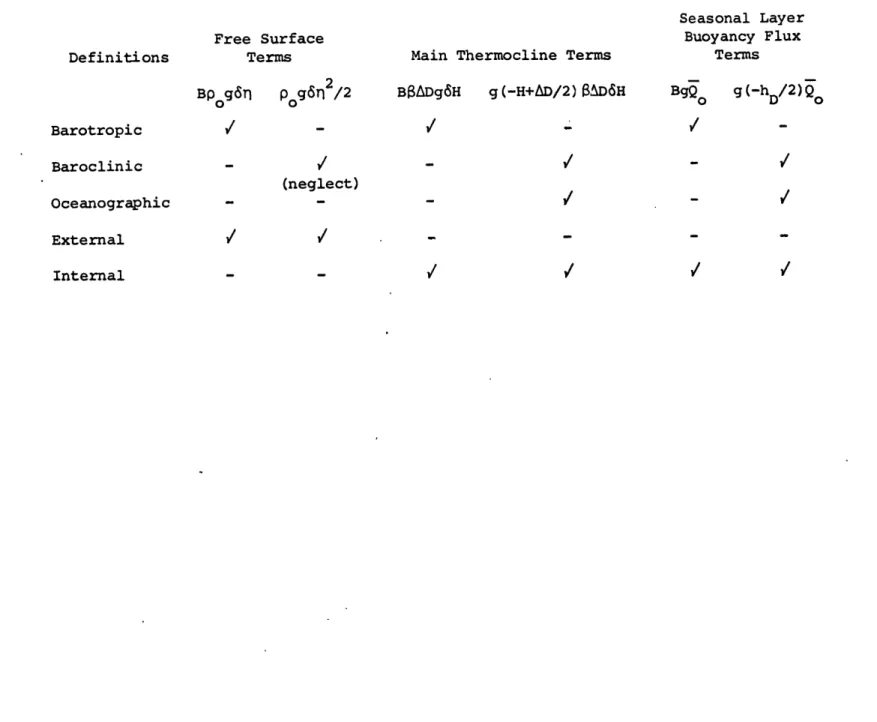
Thus the quasi-geostrophic streamfunction is proportional to the sum of a potential energy term, H, and a bottom pressure term, BPB. Fofonoff (1969) discusses a similar breakdown of the top to bottom trans-port field. Since the term arising from the bottom pressure is depth independent and is simply the bottom velocity times the total depth, he
refers to this part of the transport field as "barotropic." The depth dependent transport due to relative (to the bottom) velocities, as com-puted from the potential energy term, is referred to as baroclinic by Fofonoff (1969). It can be shown that to O(Ap/p ) the potential energy
term is equivalent t'o the oceanographic transport streamfunction, relative to the bottom, as deduced from hydrographic data. The two quantities are not exactly related because of differences in pressure and geometric coordinate derivations, althouth the total transports are equivalent for the two coordinate systems.
Both H and pB can be written explicitly in terms of our prescrip-tion since p(z) is given for all z. These integrals work out to be (refer again to Fig. 4): yh /6 h B (H3-D 3) 3 B 2 6 LS m s 2 g = g +
L h s hmY/6
+psg 2 (38) 2 h /2 h = g BB + 2 Y(h 2 - hm 2)/2 c + ps gn (39) 0 ovPlugging these results into equation (37); utilizing the fact that B, p =
constant, pLW = constant and therefore (H-D) = constant when convection does not occur; and assuming that relative to h m, hLS is constant during erosion
of the seasonal thermocline (all of these with respect to time), yields
F
h2
(
at
s
2
at
h
h
a
-y2 B(AD B$D H+ s m + p+ 0 8- --- -BAD
(H+D) DH 2m+ Y 2 at+
p nnhm at 2 at
2
p0 f
a-n
+ ) [no deep convection]where AD - H - D = constant with respect to time and we have neglected
ap 2 s 2
s B AQ) • When convection
the pieces , Ap - to O( , ) . When convection
t 2 t s h2 O
occurs, this vorticity equation becomes:
S2 H D ) 2 H D2 D }
a
(B
(H T-
D
-+p
)-+
p
2J}
ay2 St t o t 2 at 2 Bt + at 2f =- (i + PO [deep convection] gat
p
We finally simplify these into one equation in two unknowns by pulling out the pieces which depend -directly on the surface heat fluxes and are therefore assumed given by the Warren model thermodynamic equa-tions (12 ) . For the building and erosion of the seasonal thermocline:
2 S h /2 p f Q
AD
aH
a
[ s oo Qo (4)ay
2 { AD(B-H + -)7 +p B T + Qo[ B -{hm /2 ] g + ) (40)
[no deep convection]
In reaching this equation, we have also neglected the T2 term to O(n/B) and used the constancy of AD to write D = H - AD. Since h and h are
s m
known at any time from time integration of the thermodynamic equation, this is a nonlinear partial differential equation in q and H if Qo is
known.
The final form for the instance of convection is a bit differ-ent. In this case we assume that changes in the main thermocline
thickness, AD, are due solely to the surface heat losses and that they are consonant with changes in the deep mixed layer density, i.e.,
aLD 1 aPLW Q
t - '
at
-DThis implicity assumes "non-penetrative" convection in which no entrain-ment of main thermocline water into the mixed layer occurs. Rather, the diffusive interface progresses into the main thermocline just at
neutral stability by evenly cooling the mixed layer. Anati (1971) com-pares penetrative and non-penetrative models for deep convection in the Mediterranean and finds that the non-penetrative model predicts the ob-servations much more closely. If wind stirring were included in this model, some penetrative convection might be expected, at least for the shallow convection when the seasonal thermocline is eroded. For the convection associated with cooling, however, we believe, as Warren (1972) did, that non-penetrative mixing is more appropriate.
The form of the vorticity equation during deep convection works out to be:
a2 H an pfo Qo
(2
{AD(B-H + AD/2) - + pcB + Q [1 - D/2]} = ( + --- ) (41)
ay2 at o t 0 g. at 0
where now AD is not constant and D must also be computed using the thermo-dynamic equation:
aD
aH
DADaH
Qo-t at at at
SD
Although these total vorticity equations (40),(41), look complicated, it is helpful to view the left-hand side of the equations as the streamfunction (differentiated) which is composed of three
contributors: the free surface, the main thermocline, and the seasonal heat storage. Each of these contributions has a "barotropic" piece due to changes in bottom pressure, which are all multiplied by the total depth B. Each of the contributors also has a "baroclinic" piece (with the exception of theln2 term we neglected) consisting of the nonlinear potential energy terms in H and D and also Qo. The baroclinic buoyancy flux term is seen to have analogous form throughout the year, i.e.,
-(hD/2)Qo, where hD = hs, hm, and D in heating, cooling, and deep
con-vection, respectively. It is apparent that during convection larger changes in the barociinic (H) term will result for a given heat loss since then h = D is about ten times larger than h or h .
D s m
2. Lower Layer Equations
At this point we have a total top-to-bottom vorticity statement in two unknowns, n and H. As a second equation we derive a vorticity statement for the deep, constant density layer. Since this is bounded by a flat bottom and the interface H, which is one unknown, it is
suit-able for a second equation and is considerably easier to use than the layer above z = -H.
The same steps are followed as for the total equation, so only an outline of the procedure is given below.
The two-dimensional, vertically integrated vorticity equation obtained by integrating between -B and -H is:
(-L)=- f ; UL E udz.
39
Going to the quasi-geostrophic, f-plane limit gives:
a2 HL PB aPH 2 aH - H
( + B H ) = -Pf ; HL pgzdz, pH
-
pgdz .ayat ay y y o t L -B H -H
However, since p(z) - pB in this layer, this simplifies to:
a2
B 2 aH((B-H) -) = -P f
ayat ay oo at
showing the barotropic nature of this layer. Here we make a rather crude approximation to linearize this equation somewhat. We write H = H + 6H and neglect terms of O(6H/H ) in the left-hand term. This neglects varia-tions of H in latitude as well as time and thereby also neglects time mean spatial variations. We will comment further on this later. This allows us to write the lower layer vorticity equation as:
a
2aPB 2 DH
[(B-H ) -- ] = -P f
ay2
o
t
o
t
Using our prescription for bottom pressure yields:
2 2
~2 {(BH~H an P fo
aH
o2
(B-H )(
AD
T + P - + Q )} = g-ay
o
t
0
at
o
g
at
which is valid for any time of the year. To be consistent with this order of approximation we must also neglect terms of order (6H/H ) in
o
our total vorticity equation. Our final resulting set of vorticity equations is therefore:
40 2 [H -AD/2] Qo h f Tt MD o aH
+
o D oa3
o Total: ) + - ( - -) = ( + y 2 P0 B at t p 2B gB t p (42) a2 HQo
f2 Lower: 1 - o)( t(+ + ) (43) 2 B pat
at
p 9B twhere we have divided both equations by poB. It is interesting that the
2 2
natural scale which multiplies the stretching terms is f /gB = 1/X where X is the external Rossby Radius of deformation. Since our length scale in y is the same order (1000 km) as the external radius of
de-formation, it is reasonable that the two sides of these equations are comparable. It will be seen later that this scale matching is a very
III. Solution of Equations/Numerical Method
A. Form of Forcing and Boundary Conditions
The magnitude and, to some extent, the shape of the forcing we will use is based on data made available by Bunker. This will specify Q (y)
in our pair of vorticity equations, (42), (43). Since it is necessary to know the depth of the diffusive interface in computing the buoyancy flux potential energy terms in the total vorticity equation, we will also be ihtegrating Qo in time and using the time integrals of our density equation, (12),to evaluate hD. We are, therefore, using the Warren model equations, except that Qo is not a function of ps (and thereby hD
as it would normally be. Thus hD is given directly from the integral of Qo rather than being given by iteration to an equilibrium value of
the two sides of the density equation.
In Fig. 5 is shown the seasonal cycle of heating, with the annual
mean removed, for several latitudes from 100-400N averaged between 500-600W. These are from monthly averages using all the available data from 1941-1972. It is apparent from this that at the northern latitudes the seasonal signal accounts for almost all the variance about the mean, but that farther south the semiannual oscillations become the same size as the annual signal. The general diminution in amplitude to the south is also apparent. The structure of the heating function in y is more clearly shown in Fig. 6. The destructive interference between the annual and semiannual signals is again apparent to the south.
In order to solve the system (42), (43) we need four boundary condi-tions. At the southern end of our domain (20-250N) we say the forcing
actually diminishes to zero. This is done to separate the subtropics from the tropics dynamically and also because the annual signal becomes less dominant to the south. We then specify the homogeneous boundary conditions that neither the total nor the lower layer streamfunctions change at the southern end, consistent with zero forcing there. Since we don't know a priori how these quantities will respond, we are at a loss to specify more realistic southern boundary conditions.
We envision our northern boundary as the center of the eighteen degree water formation region, the subtropical gyre center, at about 350N, where meridional gradients disappear. This is consistent with the zonal velocity being identically zero at the gyre center. Because of our simplified meridional momentum equation, the meridional velocity
also goes to zero in the gyre center because the zonal acceleration there is zero. Therefore, we specify no slope boundary conditions on the total and lower layer streamfunctions. To be consistent with these homo-geneous boundary conditions, we require the forcing to have no slope at
the northern boundary also.
Of course it is rather artificial to apply boundary conditions such as these without real boundaries present. The southern condition is especially poor since the observed forcing really does not diminish to
zero. Nonetheless, these seem more adequate than periodic domain
sorts of conditions, and in the absence of prior knowledge of the system's response, the simplest homogeneous boundary conditions are at least a first step toward obtaining a unique solution to the governing equations.
Thus far, we have considered only the seasonal forcing. Since this has zero annual mean, the model will not be forced to go into deep con-vection. Rather, a seasonal thermocline will be developed in summer and
exactly erased in winter. In Warren (1972) deep convection was forced to occur by beginning in a state with excessive heat content relative to the atmospheric state. Because of the dependence of the heat flux on surface temperature,his model eventually settled into a limit cycle with no net heat loss over a year, and he obtained a deep eighteen degree water layer due to several years of late winter deep convection. In this model, our beginning state is intended to model the observed mean state, which should correspond to the limit cycle reached in Warren (1972). Thus we wouldn't expect a net yearly heat loss to occur even if we had retained the thermodynamic feedback present in Warren's model.
To investigate the response of the model to deep convection and to eighteen degree water formation, we will impose "severe" winters which result in a net heat loss over a year. Warren (1972) defined a "severe" winter as one in which there is a net decrease of about 1C in air
temperature and a net increase of about 5 knots in wind speed averaged over the six months of winter. In terms of his forcing, this resulted
in a rate of roughly 30-40 Watts/m2 additional heat loss during the winter. Observations seem to show anomalies more like 50 W/m2 , possibly as large as 100 W/m2, for heat flux variations from winter to winter. This is illustrated in Fig. 7 which shows various atmospheric and heat
flux parameters for the area 30-40*N, 50-60W for all years with avail-able data. Although the area represented contains the Gulf Stream, we expect the magnitudes of the heat flux variations to be comparable for
our northern region. It is apparent that the large negative heat fluxes in "severe"* winters are correlated with large latent heat losses. These are not always due to anomalously high winds, though the wind direction
is consistently from the northwest. The sensible heat losses, though smaller, are enhanced by anomalously cold air temperatures when the wind comes from this direction, as well as by the increased winds. Often it is the sensible flux which makes the difference between an average or
"severe" winter.
An independent method of estimating the expected heat losses is to estimate the change in heat storage after a severe winter. Referring again to Fig. 2, we approximate the change in heat storage as follows: if we say the surface temperature was lowered by approximately 0.20C in a severe winter, and this occurred over a depth range of 600 meters, the change in heat content would be about 12 kcal. If this was distributed evenly over a six month period, the average heat flux would then be roughly 30 W/m 2 very nearly the figure used by Warren (1972).
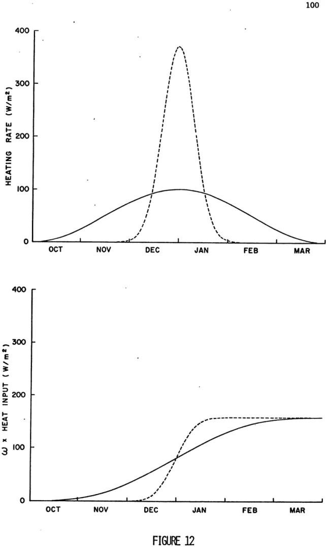
In our case studies of severe winters, we will investigate the re-sponse to a slowly varying net heat loss over the winter of about 100 Watts/m2 maximum to the north, and to a very event-oriented heat loss of larger amplitude but shorter duration. The latter is intended to model
the observed outbreaks of polar continental air in a severe winter. The amplitude of the seasonal forcing will be taken as 200 W/m2 to the north, with both the seasonal and winter anomalies diminishing to zero at the
*Here heat fluxes larger than -400 W/m2 (seasonal and mean) are con-sidered "severe" as indicated by the dashed horizontal line in Fig. 7.
southern end. Various shapes in the meridional direction will be used. as will be shown with the results obtained from the model.
B. Method of Solution
Now that boundary conditions have been defined, we can proceed to solve the governing equations (42),(43). Since the Warren model is local in nature, we wish to obtain a quasi-local form of the vorticity equations. This is accomplished by integrating both equations twice with respect to y, with the limits of integration chosen to utilize the boundary condtions explicitly. The form of the equations obtained by these y-integrations ends up being simpler to solve than the finite difference equations obtained without integration. This simplification is only possible because of the integrable form we have arrived at in
(42) and (43). If it was necessary to include the nonlinear terms neglected by dropping 6H/H terms, or to include beta effects, it would probably
0
not be to our advantage to utilize this y-integration method.
The simplest trapezoidal rule approximation will be utilized to estimate the two double integrals which result from the integration of the vortex stretching terms. There is a numerical problem with the northern, no-slope boundary condition when this form is used, however, so it is necessary to actually double the domain of interest. The no-slope condi-tion is then obtained by mirror symmetry about the midpoint of the doubled domain. Thus if we have a domain of length L, in the double domain we specify -L as the southern end, 0 as the northern end, and L as the mirror image of the southern end. The following example indicates the derivation:
yy = 0; 4(0) = 0,
4y(L)
=0 [single domain]yy= 8; (-L) = 0, (+L) = 0 [double domain]
integrating once Y y(y) - y(-L) = dy -L integrating again (y) - (-L) = dy Ody + (-L)d -L -L -L
by b.c. at -L and since
4
(-L) = a constant yY Y
(y) = dy Ody + (y+L) y (-L)
-L -L by b.c. at +L A (L) = L dy f dy + 2L (-L) = 0 -L f-L 1 L Y .) (-L) =dy J dy y(-L) 2L -L d -L final form A A (y) = dy L dy - L -L dy d . (44) -L -L -L -L
The final form obviously satisfies the boundary conditions at y = ±L. It is relatively easy to show that, if 6 is an even function about y = 0
(as it should be by mirror symmetry), the boundary condition
)
(0) = 047
By direct analogy, the double integration of (42), (43) is equivalent to 1 aH B o Qo
=
B at+
at '=)
gB t p and H f2 o aPB o aH Bat '
gB atrespectively, in (44). The equations obtained from this procedure are then:
2
h Q f Q
BAD (l - ±H (H,-AD/2) +a ( hDo o a o
p0 B at at 2B P0 gB at po 2 H BAD aH o 0 I{-(46) p at t p0 gB H
(1
-o)
B
where A I{}
dy { }dyL { } d -L -L -L -Lis a function of y coupling the left-hand side quantities, defined at that position in y, with all other points in y.
The numerical procedure utilized in the model further simplifies (45), (46) in two ways. First, as mentioned above, a trapezoidal approximation
48
is used for the double integral "I". The derivation, given in Appendix B,
gives a simple set of weights to each point, depending on the position where the equations are to be solved. Thus at a position yi the double integral is a weighted sum from all points at y. so that:
2M+1
Ii - (Ay)2 21 a..{ }. j=1
where M is the number of divisions into which the single domain is split, such that Ay = L/M , and the total number of points is 2M+1.
The second finite element simplification to (45), (46) is a time-stepping integration. Over a small time step we linearize the equations by assuming the coefficients are nearly constant, so that all the terms
(except Qo) are perfect integrals. Since Qo is given analytically, so is its integral. After each time step, all coefficients are then updated and another time-step is executed.
With these numerical approximations, over any time step 6t, we have two algebraic equations to solve at each point:
BAD (H -AD /2) hi Qoi
(1 - )6H + 6i + (1 -- )
Po B i i 2B po
(47) 2M
2+1 Q
(f 0Ay)2 a..(6n + I)P
gBo j=l 1 j P
6H +o ny 2 1 a H /(1-H-gBB) (48)