Induction Machine Parameter Identification Using LMS Algorithm Associated with a Nonlinear Adaptive Oserver

(1)

See discussions, stats, and author profiles for this publication at: https://www.researchgate.net/publication/326783858

Induction Machine Parameter Identiﬁcation Using LMS Algorithm Associated

with a Nonlinear Adaptive Observer: ICEERE 2018, 15-17 April 2018, Saidia,

Morocco

Chapter · January 2019 DOI: 10.1007/978-981-13-1405-6_68 CITATIONS 0 READS 160 5 authors, including:

Some of the authors of this publication are also working on these related projects:

Extremum Seeking and P&O Control Strategies for Achieving the Maximum Power for a PV Array: Artificial Intelligence in Renewable Energetic SystemsView project

Nonlinear Control SystemsView project Mohammed Belkheiri

Université Amar Telidji Laghouat

91PUBLICATIONS 285CITATIONS

SEE PROFILE

Ahmed Belkheiri

11PUBLICATIONS 26CITATIONS

SEE PROFILE

Mourad Boufadene

SEE PROFILE

Hamou Ait Abbas Université de Bouira

SEE PROFILE

All content following this page was uploaded by Mohammed Belkheiri on 03 January 2019. The user has requested enhancement of the downloaded file.

(2)

algorithm associated with a nonlinear adaptive observer

Mohammed Belkheiri1_{, Ahmed Belkheiri}1_{, Boufaden Mourad}2_{, Ait Abbas Hamou}2_,

and Abdlhamid Rabhi3

1_{Laboratoire de Télécommunications, Signaux et Système}

University Amar Telidji of Laghouat, PB. 37G, Ghardia Road, Laghouat, 03000, Algeria

2 _{Ecole Supérieure en Sciences Appliquées à Alger, Place des Martyrs, Alger 16001,Algérie}

3 Laboratoire Modélisation Information et Systèmes, 33 rue Saint Leu - 80039 Amiens- France m.belkheiri@lagh-univ.dz

Abstract. In this paper, we describe and evaluate a method for estimating the induction motor parameters. It is fast, efficient, and does not require special test signals or machine configuration. In addition, this method is adequate for the continuous updating of the parameters of the normal operation of the machine, so that the monitoring of the variations of the parameters is possible, we do not consider the problem of estimating the speed, but rather to simplify the problem by assuming that the speed is known. On the other hand, the speed is assumed variable, showing how the rotor flux estimates can be constructed at the same time. The Results of simulation show the effectiveness of the proposed identifi-er associated with the obsidentifi-ervidentifi-er.

Keywords: Induction machine, parameter identification, flux observer.

1 Introduction

The induction motor has become very used in various industrial applications thanks to its low cost and robustness. This type of machine has been proposed to replace hy-draulic actuators in aerospace applications and internal combustion engines [1]. Solv-ing problems related to the regulation and / or trackSolv-ing of the speed of induction mo-tors has attracted the automatic community through recent nonlinear control tech-niques such as input/output linearization, backstepping and theory of passivity. What-ever control method is used, a significant problem must be first solved which is a precise machine model with exact parameters. The uncertainties in the parameters may affect the performance of the designed control laws [2,6]. The problem is usually complicated by the fact that some state variables (i.e. the rotor flux components) are not measured or require expensive sensors for their measurement. If the flux is meas-ured, it would be relatively simpler to design a recursive identifier to estimate the motor parameters [1, 3]. Nevertheless, if the parameters of the machine are known exactly, then it would be possible to design an observer to estimate the flux. However, the common problem is much more complicated. It does not fall directly into the

(3)

2

adaptive identification framework because of the non-linearity of the dynamic model of the induction motor.

The standard methods of estimating the parameters of the induction motor include the locked rotor test, the open circuit test, and the stop frequency response test, a proce-dure is described automatically in which a sequence of these tests is performed. Each test is designed to isolate and measure a specific parameter [4].

Another procedure is described, based mainly on the identification of the transfer function of the motor at standstill. The model is then refined to account for magnetic saturation and adaptation is included to compensate for the effects of heating [5,6]. In this paper, we describe and evaluate a method for estimating induction motor pa-rameters. It is fast, efficient, and does not require special test signals or machine con-figuration. In addition, the method is adequate for the continuous updating of the pa-rameters of the normal operation of the machine, so that the monitoring of the varia-tions of the parameters is possible, we do not consider the problem of the estimate of the speed, but rather to simplify the problem by assuming that the speed is known. On the other hand, the speed is assumed variable, showing how the rotor flux esti-mates can be constructed at the same time.

The paper is organized as follows. Section II presents the standard asynchronous ma-chine modeling. The least squares identification is applied for the estimation of the electric and mechanical parameters of the motor in section III. The method for re-building flux is also detailed. Simulation and Results are presented in section IV.

2 Mathematical modelling of the induction motor

Standard models of induction machines are widely developed in the literature see [1] for example, where a suitable model for control applications is discussed. Some com-plex effects such as hysteresis, eddy currents, magnetic saturation are generally ne-glected in establishing Induction motor model for controller design. The identification algorithm presented here is based on the model expressed in a coordinate frame rotat-ing with the rotor.

𝑑𝑑𝑑𝑑𝑠𝑠𝑠𝑠 𝑑𝑑𝑑𝑑 = 1 𝜎𝜎𝜎𝜎𝑠𝑠 𝑣𝑣𝑠𝑠𝑠𝑠− 𝛾𝛾𝛾𝛾𝑠𝑠𝑠𝑠+ 𝛽𝛽 𝑇𝑇𝑟𝑟𝜓𝜓𝑟𝑟𝑠𝑠+ 𝑛𝑛𝑝𝑝 𝛽𝛽𝛽𝛽𝜓𝜓𝑟𝑟𝑟𝑟+ 𝑛𝑛𝑝𝑝𝛽𝛽𝛾𝛾𝑠𝑠𝑟𝑟 (1) 𝑑𝑑𝑑𝑑𝑠𝑠𝑠𝑠 𝑑𝑑𝑑𝑑 = 1 𝜎𝜎𝜎𝜎𝑠𝑠𝑣𝑣𝑠𝑠𝑟𝑟− 𝛾𝛾𝛾𝛾𝑠𝑠𝑟𝑟+ 𝛽𝛽 𝑇𝑇𝑟𝑟𝜓𝜓𝑟𝑟𝑟𝑟− 𝑛𝑛𝑝𝑝𝛽𝛽𝛽𝛽𝜓𝜓𝑟𝑟𝑠𝑠− 𝑛𝑛𝑝𝑝𝛽𝛽𝛾𝛾𝑠𝑠𝑠𝑠 (2) 𝑑𝑑𝑑𝑑𝑟𝑟𝑠𝑠 𝑑𝑑𝑑𝑑 = 𝑀𝑀 𝑇𝑇𝑟𝑟𝛾𝛾𝑠𝑠𝑠𝑠− 1 𝑇𝑇𝑟𝑟 𝜓𝜓𝑟𝑟𝑠𝑠 (3) 𝑑𝑑𝑑𝑑𝑟𝑟𝑠𝑠 𝑑𝑑𝑑𝑑 = 𝑀𝑀 𝑇𝑇𝑟𝑟 𝛾𝛾𝑠𝑠𝑟𝑟 − 1 𝑇𝑇𝑟𝑟 𝜓𝜓𝑟𝑟𝑟𝑟 (4) 𝑑𝑑𝑑𝑑 𝑑𝑑𝑑𝑑 = 2𝑀𝑀𝑀𝑀𝑝𝑝 𝐽𝐽𝜎𝜎𝑟𝑟 𝑀𝑀𝑝𝑝ℎ �𝛾𝛾𝑠𝑠𝑟𝑟𝜓𝜓𝑟𝑟𝑠𝑠− 𝛾𝛾𝑟𝑟𝑠𝑠𝜓𝜓𝑟𝑟𝑟𝑟� − 𝜏𝜏𝐿𝐿 𝐽𝐽 (5)

In the above model, the angular velocity of the rotor is denoted as ω and Nph is the number of phases. The unknown parameters of the model are the five electrical

(4)

pa-rameters, Rs and Rr (stator and rotor resistors), M (the mutual inductance), Ls and Lr (stator and rotor inductors), and the two mechanical parameters, J (rotor inertia) and

τL (load torque). The symbols 𝑇𝑇_𝑟𝑟= 𝜎𝜎𝑟𝑟 𝑅𝑅𝑟𝑟, 𝜎𝜎 = 1 − 𝑀𝑀2 𝜎𝜎𝑎𝑎𝜎𝜎𝑟𝑟, 𝛽𝛽 = 𝑀𝑀 𝜎𝜎𝜎𝜎𝑠𝑠𝜎𝜎𝑟𝑟, and 𝛾𝛾 = 𝑅𝑅𝑠𝑠 𝜎𝜎𝜎𝜎𝑠𝑠+ 𝑀𝑀2𝑅𝑅𝑟𝑟 𝜎𝜎𝜎𝜎𝑠𝑠𝜎𝜎𝑟𝑟2 have been

used to simplify expressions. 𝑇𝑇_𝑟𝑟 is the constant rotor time and 𝜎𝜎 is the total leakage-factor. Manipulating the induction motor model (1 to 5) to get a simplified model where the unknown parameters can be linearly isolated as follows:

𝑑𝑑𝑑𝑑𝑠𝑠𝑠𝑠 𝑑𝑑𝑑𝑑 + 𝛾𝛾𝛾𝛾𝑠𝑠𝑠𝑠− 𝛽𝛽 𝑇𝑇𝑟𝑟𝜓𝜓𝑟𝑟𝑠𝑠− 𝑛𝑛𝑝𝑝𝛽𝛽𝛽𝛽𝜓𝜓𝑟𝑟𝑟𝑟− 𝑛𝑛𝑝𝑝𝛽𝛽𝛾𝛾𝑠𝑠𝑟𝑟= 1 𝜎𝜎𝜎𝜎𝑠𝑠𝑣𝑣𝑠𝑠𝑠𝑠 (6) 𝑑𝑑𝑑𝑑𝑠𝑠𝑠𝑠 𝑑𝑑𝑑𝑑 + 𝛾𝛾𝛾𝛾𝑠𝑠𝑟𝑟− 𝛽𝛽 𝑇𝑇𝑟𝑟 𝜓𝜓𝑟𝑟𝑟𝑟− 𝑛𝑛𝑝𝑝𝛽𝛽𝛽𝛽𝜓𝜓𝑟𝑟𝑠𝑠+ 𝑛𝑛𝑝𝑝𝛽𝛽𝛾𝛾𝑠𝑠𝑠𝑠 = 1 𝜎𝜎𝜎𝜎𝑠𝑠𝑣𝑣𝑠𝑠𝑟𝑟 (7)

Taking the first derivatives of equations (6) and (7) and after some mathematical ma-nipulations we can get

1 𝜎𝜎𝜎𝜎𝑠𝑠 𝑑𝑑𝑑𝑑𝑠𝑠𝑠𝑠 𝑑𝑑𝑑𝑑 + 1 𝑇𝑇𝑟𝑟𝜎𝜎𝜎𝜎𝑠𝑠𝑣𝑣𝑠𝑠𝑠𝑠− 𝑛𝑛𝑝𝑝𝛽𝛽 � 1 𝑇𝑇𝑟𝑟+ 𝛽𝛽𝑀𝑀 𝑇𝑇𝑟𝑟� 𝛾𝛾𝑠𝑠𝑟𝑟= 𝑑𝑑2𝑑𝑑𝑠𝑠𝑠𝑠 𝑑𝑑𝑑𝑑2 + �𝛾𝛾 +_𝑇𝑇1_𝑟𝑟�𝑑𝑑𝑑𝑑_{𝑑𝑑𝑑𝑑}𝑠𝑠𝑠𝑠+ �_𝑇𝑇𝛾𝛾_𝑟𝑟−𝛽𝛽𝑀𝑀_𝑇𝑇_𝑟𝑟2� 𝛾𝛾𝑠𝑠𝑠𝑠 − 𝑛𝑛𝑝𝑝�𝛾𝛾𝑠𝑠𝑟𝑟+ 𝛽𝛽𝜓𝜓𝑟𝑟𝑟𝑟�𝑑𝑑𝑑𝑑_{𝑑𝑑𝑑𝑑}- 𝑛𝑛𝑝𝑝𝛽𝛽𝑑𝑑𝑑𝑑_{𝑑𝑑𝑑𝑑}𝑠𝑠𝑠𝑠 (8) 1 𝜎𝜎𝜎𝜎𝑠𝑠 𝑑𝑑𝑑𝑑𝑠𝑠𝑠𝑠 𝑑𝑑𝑑𝑑 + 1 𝑇𝑇𝑟𝑟𝜎𝜎𝜎𝜎𝑠𝑠𝑣𝑣𝑠𝑠𝑟𝑟= 𝑑𝑑2_𝑑𝑑_{𝑠𝑠𝑠𝑠} 𝑑𝑑𝑑𝑑2 + �𝛾𝛾 +_𝑇𝑇1_𝑟𝑟� 𝑑𝑑𝑑𝑑𝑠𝑠𝑠𝑠 𝑑𝑑𝑑𝑑 + � 𝛾𝛾 𝑇𝑇𝑟𝑟− 𝛽𝛽𝑀𝑀 𝑇𝑇𝑟𝑟2� 𝛾𝛾𝑠𝑠𝑟𝑟+ 𝑛𝑛𝑝𝑝𝛽𝛽 � 1 𝑇𝑇𝑟𝑟+ 𝛽𝛽𝑀𝑀 𝑇𝑇𝑟𝑟� 𝛾𝛾𝑠𝑠𝑠𝑠+ 𝑛𝑛𝑝𝑝(𝛾𝛾𝑠𝑠𝑠𝑠+ 𝛽𝛽𝜓𝜓𝑟𝑟𝑠𝑠)𝑑𝑑𝑑𝑑_{𝑑𝑑𝑑𝑑} + 𝑛𝑛𝑝𝑝𝛽𝛽𝑑𝑑𝑑𝑑_{𝑑𝑑𝑑𝑑}𝑠𝑠𝑠𝑠 (9) This model can be written as:

𝑑𝑑2_{𝛾𝛾𝑠𝑠𝑠𝑠} 𝑑𝑑𝑑𝑑2 + 𝜃𝜃1 𝑑𝑑𝛾𝛾𝑠𝑠𝑠𝑠 𝑑𝑑𝑑𝑑 + 𝜃𝜃2𝛾𝛾𝑠𝑠𝑠𝑠− 𝜃𝜃3𝑛𝑛𝑝𝑝𝛽𝛽𝛾𝛾𝑠𝑠𝑟𝑟− 𝑛𝑛𝑝𝑝𝛽𝛽 𝑑𝑑𝛾𝛾𝑠𝑠𝑟𝑟 𝑑𝑑𝑑𝑑 = 𝜃𝜃4 𝑑𝑑𝑣𝑣𝑠𝑠𝑠𝑠 𝑑𝑑𝑑𝑑 + 𝜃𝜃5𝑣𝑣𝑠𝑠𝑠𝑠 (10) 𝑑𝑑2_{𝛾𝛾𝑠𝑠𝑟𝑟} 𝑑𝑑𝑑𝑑2 + 𝜃𝜃1 𝑑𝑑𝛾𝛾𝑠𝑠𝑠𝑠 𝑑𝑑𝑑𝑑 + 𝜃𝜃2𝛾𝛾𝑠𝑠𝑟𝑟+ 𝜃𝜃3𝑛𝑛𝑝𝑝𝛽𝛽𝛾𝛾𝑠𝑠𝑠𝑠+ 𝑛𝑛𝑝𝑝𝛽𝛽 𝑑𝑑𝛾𝛾𝑠𝑠𝑠𝑠 𝑑𝑑𝑑𝑑 = 𝜃𝜃4 𝑑𝑑𝑣𝑣𝑠𝑠𝑟𝑟 𝑑𝑑𝑑𝑑 + 𝜃𝜃5𝑣𝑣𝑠𝑠𝑟𝑟 (11) where 𝜃𝜃1= 𝛾𝛾 +_𝑇𝑇1 𝑟𝑟 , 𝜃𝜃2= 𝛾𝛾 𝑇𝑇𝑟𝑟 − 𝛽𝛽𝑀𝑀 𝑇𝑇_𝑟𝑟2, 𝜃𝜃3=_𝑇𝑇1_𝑟𝑟+𝛽𝛽𝑀𝑀_𝑇𝑇_𝑟𝑟 , 𝜃𝜃4=_{𝜎𝜎𝜎𝜎}1_𝑠𝑠 , 𝜃𝜃5=_{𝜎𝜎𝜎𝜎}1_𝑠𝑠_𝑇𝑇_𝑟𝑟

To estimate the physical parameters, we can use 𝑅𝑅𝑠𝑠=𝜃𝜃2 𝜃𝜃5, 𝐿𝐿𝑠𝑠= 𝜃𝜃3 𝜃𝜃5, 𝜎𝜎 = 𝜃𝜃5 𝜃𝜃3𝜃𝜃4, 𝑇𝑇𝑟𝑟= 𝜃𝜃4 𝜃𝜃5

The model can also be expressed in matrix as shown below:

�− 𝑑𝑑𝛾𝛾𝑠𝑠𝑠𝑠 𝑑𝑑𝑑𝑑 −𝛾𝛾𝑠𝑠𝑠𝑠 𝑛𝑛𝑝𝑝𝛽𝛽𝛾𝛾𝑠𝑠𝑟𝑟 −𝑑𝑑𝛾𝛾𝑠𝑠𝑟𝑟 𝑑𝑑𝑑𝑑 −𝛾𝛾𝑠𝑠𝑟𝑟 −𝑛𝑛𝑝𝑝𝛽𝛽𝛾𝛾𝑠𝑠𝑠𝑠 𝑑𝑑𝑣𝑣𝑠𝑠𝑠𝑠 𝑑𝑑𝑑𝑑 𝑑𝑑𝑣𝑣𝑠𝑠𝑟𝑟 𝑑𝑑𝑑𝑑 𝑣𝑣_{𝑣𝑣𝑠𝑠𝑟𝑟}𝑠𝑠𝑠𝑠 � ⎝ ⎜ ⎛ 𝜃𝜃1 𝜃𝜃2 𝜃𝜃3 𝜃𝜃4 𝜃𝜃5⎠ ⎟ ⎞ = ⎝ ⎛ 𝑑𝑑2_{𝛾𝛾𝑆𝑆𝑠𝑠} 𝑑𝑑𝑑𝑑2 − 𝑛𝑛𝑝𝑝𝛽𝛽𝑑𝑑𝛾𝛾_{𝑑𝑑𝑑𝑑}𝑆𝑆𝑟𝑟 𝑛𝑛𝑝𝑝𝛽𝛽𝑑𝑑𝛾𝛾𝑆𝑆𝑠𝑠_{𝑑𝑑𝑑𝑑 +}𝑑𝑑_{𝑑𝑑𝑑𝑑}2𝛾𝛾𝑠𝑠𝑟𝑟₂ _⎠ ⎞ (12) This linear form of the motor model allows direct application of a least squares identification algorithm to estimate electrical parameters.

Using equation (12) and defining the error vector as

(5)

4

where 𝝋𝝋(𝑘𝑘) represents the regressor vector, 𝜽𝜽 the vector

parameters to be identified and 𝜀𝜀(𝑘𝑘) the error of equation written in the general form of prediction error. 𝝋𝝋𝐓𝐓_{(𝑘𝑘) = �}− 𝑑𝑑𝛾𝛾𝑠𝑠𝑠𝑠 𝑑𝑑𝑑𝑑 −𝛾𝛾𝑠𝑠𝑠𝑠 𝑛𝑛𝑝𝑝𝛽𝛽𝛾𝛾𝑠𝑠𝑟𝑟 −𝑑𝑑𝛾𝛾_{𝑑𝑑𝑑𝑑}𝑠𝑠𝑟𝑟 −𝛾𝛾𝑠𝑠𝑟𝑟 −𝑛𝑛𝑝𝑝𝛽𝛽𝛾𝛾𝑠𝑠𝑠𝑠 𝑑𝑑𝑣𝑣𝑠𝑠𝑠𝑠 𝑑𝑑𝑑𝑑 𝑑𝑑𝑣𝑣𝑠𝑠𝑟𝑟 𝑑𝑑𝑑𝑑 𝑣𝑣𝑠𝑠𝑠𝑠_𝑣𝑣_{𝑠𝑠𝑟𝑟} � 𝜽𝜽 = ⎝ ⎜ ⎛ 𝜃𝜃1 𝜃𝜃2 𝜃𝜃3 𝜃𝜃4 𝜃𝜃5⎠ ⎟ ⎞ , 𝒚𝒚(𝑘𝑘) = ⎝ ⎛ 𝑑𝑑2_𝛾𝛾 𝑆𝑆𝑠𝑠 𝑑𝑑𝑑𝑑2 − 𝑛𝑛𝑝𝑝𝛽𝛽 𝑑𝑑𝛾𝛾𝑆𝑆𝑟𝑟 𝑑𝑑𝑑𝑑 𝑛𝑛𝑝𝑝𝛽𝛽𝑑𝑑𝛾𝛾𝑆𝑆𝑠𝑠_{𝑑𝑑𝑑𝑑 +}𝑑𝑑_{𝑑𝑑𝑑𝑑}2𝛾𝛾𝑠𝑠𝑟𝑟₂ _⎠ ⎞

By accumulating N measurements, for example at the discrete instants k = 1, ... N, the equation (13) gives in matrix form:

⎝ ⎜ ⎛ 𝜀𝜀(1) 𝜀𝜀(2) ⋮ ⋮ 𝜀𝜀(𝑁𝑁)⎠ ⎟ ⎞ = ⎝ ⎜ ⎛ 𝑦𝑦(1) 𝑦𝑦(2) ⋮ ⋮ 𝑦𝑦(𝑁𝑁)⎠ ⎟ ⎞ − ⎝ ⎜ ⎛ 𝝋𝝋𝑇𝑇₍₁₎ 𝝋𝝋𝑇𝑇₍₂₎ ⋮ ⋮ 𝝋𝝋𝑇𝑇_{(𝑁𝑁)⎠} ⎟ ⎞ 𝜽𝜽 (14) ℇ = 𝒀𝒀 − Φ𝜽𝜽 (15) The quadratic prediction error is as follows:

min 𝐽𝐽 = � 𝜀𝜀2_(𝑘𝑘) 𝑁𝑁 𝑘𝑘=1

= ℇT_ℇ The minimization of the quadratic error gives

𝜽𝜽� = (Φ𝑇𝑇_Φ)−1_Φ𝑇𝑇_{𝑌𝑌 (16)}

3 Flux Adaptive Observer Design

Note that the need to have flux measurements is avoided by the assumption that the speed varies slowly. This is an advantage because flux measurements, which require sensors near the gap, are not practical to obtain. A disadvantage is that derivatives from there currents are needed. These can be reconstructed by filtered differentiation. In this paper an observer is designed to reconstruct the flux from the available current and the parameters identified in the precedent section.

First an observer is designed for the stator subsystem: � 𝑑𝑑𝑑𝑑𝑆𝑆𝑠𝑠 𝑑𝑑𝑑𝑑 𝑑𝑑𝑑𝑑𝑆𝑆𝑠𝑠 𝑑𝑑𝑑𝑑 � = �−𝛾𝛾 𝛽𝛽 𝑇𝑇𝑅𝑅 0 −1_𝑇𝑇 𝑅𝑅 � � 𝛾𝛾_{𝜓𝜓𝑆𝑆𝑠𝑠}𝑆𝑆𝑠𝑠� + �𝜎𝜎𝜎𝜎1𝑠𝑠 0� 𝑢𝑢𝑆𝑆𝑠𝑠+ �𝜂𝜂 𝑝𝑝𝛽𝛽𝛽𝛽𝜓𝜓𝑅𝑅𝑟𝑟+ 𝜂𝜂𝑝𝑝𝛽𝛽𝛾𝛾𝑆𝑆𝑟𝑟 0 � (17) 𝑦𝑦𝑠𝑠𝑠𝑠= (1 0) �𝛾𝛾𝑆𝑆𝑠𝑠 𝜓𝜓𝑆𝑆𝑠𝑠�

(6)

Let us parametrize the above subsystem considering the linear part and a nonlinear function 𝑓𝑓 linearly parametrized with unknown parameters as follows:

𝐴𝐴 = �−𝛾𝛾 𝛽𝛽 𝑇𝑇𝑅𝑅 0 −1_𝑇𝑇 𝑅𝑅 � , 𝐵𝐵 = �𝜎𝜎𝜎𝜎1𝑠𝑠 0� , 𝑓𝑓 = �𝜂𝜂 𝑝𝑝𝛽𝛽𝛽𝛽𝜓𝜓𝑅𝑅𝑟𝑟+ 𝜂𝜂𝑝𝑝𝛽𝛽𝛾𝛾𝑆𝑆𝑟𝑟 0 � , 𝐶𝐶 = (1 0)

The adaptive observer is designed to take the measured stator current to reconstruct the state vector using:

𝑥𝑥�̇ = 𝐴𝐴𝑥𝑥� + 𝑓𝑓(𝑢𝑢, 𝑦𝑦) + 𝐵𝐵𝐵𝐵𝜃𝜃� + 𝐿𝐿(𝑦𝑦 − 𝐶𝐶𝑥𝑥�)

where 𝑥𝑥� is the estimated state vector and the 𝜃𝜃� is the estimated parameters and L is a tuning gain of the linear part of the observer.

𝑥𝑥̇ = 𝐴𝐴𝑥𝑥 + 𝐵𝐵(𝑢𝑢, 𝑦𝑦) + 𝑓𝑓

𝑥𝑥�̇ = 𝐴𝐴𝑥𝑥� + 𝐵𝐵𝑢𝑢 + 𝑓𝑓̂ + 𝐿𝐿(𝐶𝐶𝑥𝑥 − C𝑥𝑥�)

Defining 𝑒𝑒 = 𝑥𝑥 − 𝑥𝑥� as the error between the actual and the estimated state vector; and 𝜃𝜃� = 𝜃𝜃 − 𝜃𝜃� as the parameter estiation error,

Using the Lyapunov candidate:

𝑉𝑉 = 𝑒𝑒𝑇𝑇_{𝑃𝑃𝑒𝑒 + 𝜃𝜃�}𝑇𝑇_𝛾𝛾−1_𝜃𝜃�

Where 𝛾𝛾 is a diagonal positive definite adaptation gain matrix, and P, Q are semi-positive definite matrices satisfying the algebraic Lyapunov matrix equation:

𝐴𝐴𝑇𝑇_{𝑃𝑃 + 𝑃𝑃𝐴𝐴 = −𝑄𝑄 (18)} Defining the closed loop matrix 𝐴𝐴𝑐𝑐 = 𝐴𝐴 − 𝐿𝐿𝐶𝐶 and based on equation (17), the er-ror dynamics can be expressed as:

𝑒𝑒̇ = 𝐴𝐴𝑐𝑐𝑒𝑒 + 𝐵𝐵𝐵𝐵𝜃𝜃�

The derivative of the Lyapunov equation can be given as:

𝑉𝑉̇ = 𝑒𝑒̇𝑇𝑇_{𝑃𝑃𝑒𝑒 + 𝑒𝑒}𝑇𝑇_{𝑃𝑃𝑒𝑒̇ + 𝜃𝜃�}𝑇𝑇_𝛾𝛾−1_{𝜃𝜃� + 𝜃𝜃�}̇ 𝑇𝑇_𝛾𝛾−1_{𝜃𝜃�̇}₍₁₉₎ Applying the parametrization for the stator system we can derive the stator subsys-tem observer as:

𝑑𝑑𝚤𝚤̂𝑆𝑆𝑠𝑠 𝑑𝑑𝑑𝑑 = 𝑢𝑢𝑆𝑆𝑠𝑠 𝜎𝜎𝜎𝜎𝑠𝑠− 𝛾𝛾𝛾𝛾𝑆𝑆𝑠𝑠+ 𝛽𝛽 𝑇𝑇𝑅𝑅𝜓𝜓�𝑅𝑅𝑠𝑠+ 𝜂𝜂𝑝𝑝𝛽𝛽𝛽𝛽�𝜓𝜓𝑅𝑅𝑟𝑟+ 𝜂𝜂𝑝𝑝𝛽𝛽�𝛾𝛾𝑆𝑆𝑟𝑟 (20) 𝑑𝑑𝑑𝑑�𝑅𝑅𝑠𝑠 𝑑𝑑𝑑𝑑 = 𝑀𝑀 𝑇𝑇𝑅𝑅𝛾𝛾𝑆𝑆𝑠𝑠− 1 𝑇𝑇𝑅𝑅𝜓𝜓�𝑅𝑅𝑠𝑠 (21)

and the error dynamics 𝑒𝑒̇ = 𝑥𝑥̇ − 𝑥𝑥�̇ = ⎝ ⎛ 𝑑𝑑𝛾𝛾𝑆𝑆𝑠𝑠 𝑑𝑑𝑑𝑑 − 𝑑𝑑𝚤𝚤̂𝑆𝑆𝑠𝑠 𝑑𝑑𝑑𝑑 𝑑𝑑𝜓𝜓𝑆𝑆𝑠𝑠 𝑑𝑑𝑑𝑑 − 𝑑𝑑𝜓𝜓�𝑆𝑆𝑠𝑠 𝑑𝑑𝑑𝑑 ⎠ ⎞ = ⎝ ⎜ ⎛ 𝑢𝑢𝑆𝑆𝑠𝑠 𝜎𝜎𝐿𝐿𝑠𝑠− 𝛾𝛾𝛾𝛾𝑆𝑆𝑠𝑠+ 𝛽𝛽 𝑇𝑇𝑅𝑅𝜓𝜓𝑅𝑅𝑠𝑠+ 𝜂𝜂𝑝𝑝𝛽𝛽𝛽𝛽𝜓𝜓𝑅𝑅𝑟𝑟+ 𝜂𝜂𝑝𝑝𝛽𝛽𝛾𝛾𝑆𝑆𝑟𝑟− 𝑑𝑑𝚤𝚤̂𝑆𝑆𝑠𝑠 𝑑𝑑𝑑𝑑 𝑀𝑀 𝑇𝑇𝑅𝑅𝛾𝛾𝑆𝑆𝑠𝑠− 1 𝑇𝑇𝑅𝑅𝜓𝜓𝑅𝑅𝑠𝑠− 𝑑𝑑𝜓𝜓�𝑆𝑆𝑠𝑠 𝑑𝑑𝑑𝑑 _⎠ ⎟ ⎞

(7)

6

4 Simulation Results

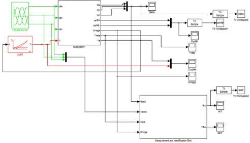
In order to test the identification method presented in this chapter, a model of the machine was constructed in the Simulation environment Matlab / 2015b. The figure summarizes the simulation scheme

Figure 1. Simulation of the Induction machine

The machine was simulated in the rotor coordinate system where the system dy-namics were divided into three interconnected subsystems (mechanical system, rotor flow system and stator current)

(8)

We considered a 1/2 KW squirrel cage asynchronous motor with following param-eters [1]:

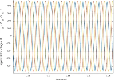
Vmax = 466.7; fr = 50; f = 0 np = 2; ph = 3; Rr = 8.6 Rs = 9.7; Lr = 0.67 Ls = 0.67; M = 0.64 Lm = M; sigma = 0.0875 J = 0.011, f = 0.001; TL = 3.7 The applied voltages are a balanced three phase voltage with a frequency of 50 Hz.

Figure 3. Applied voltages

Figure 4 : Measured currents

0.05 0.1 0.15 0.2 0.25 time (sec) -400 -300 -200 -100 0 100 200 300 400

applied stator voltages, U

Sa , U Sb , U Sc V 0 0.2 0.4 0.6 0.8 1 1.2 1.4 1.6 1.8 2 time (sec) -25 -20 -15 -10 -5 0 5 10 15 20 25 stator currents, i sx i sy A

(9)

8

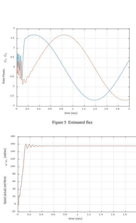
Figure 5 Estimated flux

Figure 5 : Angular velocity (actual and identified) The identified mathematical parameters are:

𝜽𝜽 = ⎝ ⎜ ⎛ 𝜃𝜃1= 263,980 𝜃𝜃2= 115.701 𝜃𝜃3= 66.9488 𝜃𝜃4= 15.69561 𝜃𝜃5= 99.09449⎠ ⎟ ⎞ 0 0.2 0.4 0.6 0.8 1 1.2 1.4 1.6 1.8 2 time (sec) -2 -1.5 -1 -0.5 0 0.5 1 1.5 2 Rotor Fluxes, rx ry 0 0.2 0.4 0.6 0.8 1 1.2 1.4 1.6 1.8 2 time (sec) -20 0 20 40 60 80 100 120 140 160 180

Speed (actual) and filtred,

f

(10)

Table 1 shows that the identified parameters are very close to the real values. The differences may be due to the conditions of use for the identification of the parameters of the IM are different from those defined by the manufacturer.

Table 1. The actual and identified electrical parameters.

Parameter Current value Estimated value

Rs 9.6999 Ω 11.675 Ω

Ls 0.6700 mH 0.6756 mH

Sigma 0.0875 0.0943

Tr 0.1491 0.1583

5 Conclusion

The aim of this paper is to propose a simple parametric identification method for the induction machine. through Simulink simulation under MATLAB, the model identi-fied by the proposed approache combined with flux estimator were veriidenti-fied and vali-dated. This study shows that: - The parameters of the machine depend on the operat-ing point and therefore the measurement conditions, - The identification results are satisfactory for a simulation of the behavior of the machine, conversely, they are in-sufficient for its control and diagnosis.

References

1. Chiasson, John. “Modeling and High-Performance Control of Electric Machines”, in: John Wiley & Sons, New Jersey, 2005.

2. Rebaia Chergui, Identification des paramètres d’un moteur asynchrone , Master thesisin electrotechnical engineering, University of Batna – Dec. 2014.

3. Mourad Boufadene , Mohammed Belkheiri , “Abdelhamid Rabhi, Adaptive nonlinear ob-server augmented by radial basis neural network for a nonlinear sensorless control of an induction machine”, International Journal of Automation and Control, Vol 12.

4. J. Stephan, M. Bodson and J. Chiasson, "Real-time estimation of the parameters and fluxes of induction motors," Conference Record of the 1992 IEEE Industry Applications Society Annual Meeting, Houston, TX, 1992, pp. 578-585 vol.1. N° 1, Jan 2018.

5. Stephan, M. Bodson and J.Chiasson, “Real-time estimation of the parameters and fluxes of induction Motor”, IEEE Transactions on industry applications 30 (3), 746-759, 1994. 6. Hamou Ait Abbas, Mohammed Belkheiri and Boubakeur Zegnini, “Feedback linearisation

control of an induction machine augmented by single-hidden layer neural networks”, In-ternational Journal of Control, Volume 89, Issue 1, 2016.

View publication stats View publication stats