Achieving and sustaining an optimal product portfolio in the healthcare industry through SKU rationalization, complexity costing, and dashboards

Achieving and Sustaining an Optimal Product Portfolio in the Healthcare

Industry through SKU Rationalization, Complexity Costing, and Dashboards

By David Hilliard

B.S. Electrical, Computer, and Systems Engineering Rensselaer Polytechnic Institute, 2003

SUBMITTED TO THE MIT SLOAN SCHOOL OF MANAGEMENT AND THE ENGINEERING SYSTEMS DIVISION IN PARTIAL FULFILLMENT OF THE REQUIREMENTS FOR THE

DEGREES OF

MASTER OF BUSINESS ADMINISTRATION AND

MASTER OF SCIENCE IN ENGINEERING SYSTEMS

IN CONJUNCTION WITH THE LEADERS FOR GLOBAL OPERATIONS PROGRAM AT THE

MASSACHUSETTS INSTITUTE OF TECHNOLOGY

ARCHIVES

MASSACHUSETTS INSTII

JUNE 2012 OF TECHNOLOGY

0 2012 David J. Hilliard. All rights reserved.

_{JUN 14 2012}

and to distribute publicly paper and electronic

LIBRARIES

copies of this thesis document in whole or in part in any medium now known or hereafter created.

Signature of Author

Engineering Systems Division, MIT Sloan School of Management May 11, 2012 Certified by

David Simchi-Levi, Thesis Supervisor Professor of Civil and Environmental Engineering and Engineering Systems Co-Director, Leaders For Globpl Operations aqd Systempesign and Management Programs Certified by

Slcott

Accepted by

I deWeck, Chair, Engineering Systems Education Committee Associate Professor of Aerorgutics and Astgojautics and Engineering Systems

Accepted by

( Maura 1. Herson, Directo77MBA Program MIT Sloan School of Management

Achieving and Sustaining an Optimal Product Portfolio in the Healthcare

Industry through SKU Rationalization, Complexity Costing, and Dashboards

by David Hilliard

Submitted to the MIT Sloan School of Management and the Engineering Systems Division on May 11, 2012 in Partial Fulfillment of the Requirements for the Degrees of Master of Business Administration and

Master of Science in Engineering Systems

Abstract

After years of new product launches, and entry into emerging markets, Company X, a healthcare company, has seen its product portfolio proliferate and bring costly complexity into its operations. Today, Company X seeks to achieve and sustain an optimal product offering that meets their customers' needs. Through a six-month research effort, we develop a process for stock-keeping-unit (SKU) rationalization to reduce SKU complexity while maintaining sales volumes. We, also, implement operational models to compute complexity costs associated with SKU complexity and employ SKU portfolio dashboards to monitor SKU development and govern SKU creation.

This thesis discusses a process for applying these tools to any healthcare company. Through two case studies, we apply the rationalization process on one pilot brand and develop a dashboard to improve product portfolio management. We expect that the SKU rationalization process will release 38% of avoidable costs associated with the pilot brand. These case studies also provide insight into how to correctly diagnose the cost reduction opportunity associated with SKU complexity, as well as methods for a step-change improvement in lead-times and cost-reduction. Lastly, removal of complexity provides

flexibility to capture other business opportunities.

Thesis Supervisor: David Simchi-Levi

Title: Professor of Civil and Environmental Engineering and Engineering Systems

Co-Director, Leaders For Global Operations and System Design and Management Programs Thesis Supervisor: Scott Keating

Acknowledgments

Through my six-months of research, I had the pleasure of working with an outstanding and motivated team. I would first like to recognize my supervisor, GM, who was a pleasure to work for and to learn from. Also, I would like to thank BR and his strong support. I would have not been able to perform the analysis in this thesis without his help. Similarly, UK and TP were extremely helpful advisors throughout my tenure at Company X. My internship was a great learning experience and a pleasure to work with all members of the operations team. A special thanks to TM, AV, DB, CE, and GB.

I would also like to thank all those associated with the Leaders for Global Operations program and the Boeing Sponsorship program. These last two years have been an amazing experience. I have learned so much about leadership and self-improvement while fulfilling my passion for operations management. Further, my LGO classmates have made this time full of laughs and great times. Specifically, I would like to thank LL and MA for some great memories during the six months.

Thank you to both of my advisors, Prof. Scott Keating and Prof. David Simchi-Levi, for their strong support and insight during my internship and the development of this thesis. Specifically, I would like to thank Scott for his site visit and thanks to David for his operations management framework that I applied to this thesis.

Lastly, I would like to thank those closest to me. First, to my girlfriend, Tricia Bealer - thank you so much for your unending love and support that I could not live without. To my siblings - Jim, Kate, Mike,

and Brie - thank you for a lifetime of guidance. To my dad, thank you for your constant encouragement that continues to inspire me.

And to my mom who passed during my research, thank you for your motivation and love that has brought me to where I am today.

Table of Contents

1.2 Problem Statem ent... 11

1.3 H y p o th esis ... 1 1 1.4 Thesis Outline ... 12

2 Literature Review ... 13

2.1 Effects of Product Complexity ... 14

3 Costing System Analysis ... 16

4 SKU Optimization Process for Healthcare Companies ... 18

4 .1 O v erv iew ... 18

4 .2 M e tric s ... 18

4 .3 R equ irem en ts ... 2 0 4.4 Implementation Process... 20

5 Case Study - SK U Rationalization on a Com pany X Brand... 50

5.1 Background... 50

5.2 Objectives ... 50

5.3 Approach... 51

5.4 Recom m endations... 65

6 Case Study - Com pany X SKU Portfolio D ashboard ... 68

6.1 SKU Portfolio M onitoring ... 68

6.2 SKU Governance Dashboard... 70

6.3 Recom m endations... 71

7 Conclusions and Next Steps ... 72

7.1 N ext Steps for Com pany X ... 73

List of Figures

Figure 1. Perumal's three types of complexity [1]... 13

Figure 2. Pasche's necessary and non-necessary product complexity [18]... 13

Figure 3. Arthur D. Little findings on the effects of complexity across the value chain [3]... 14

Figure 4. Perumal's depiction of total safety stock as a function of product variety for different levels of d em an d v ariation ... 15

Figure 5. Example comparison of margin vs. sales trend over 3 years vs. SKU complexity of brand p o rtfo lio ... 2 2 Figure 6. SKU complexity tree with a highlighted market segment... 24

Figure 7. Priority markets identified by pareto principle (Each color represents a different market)... 25

Figure 8. Packaging type vs. market segment sales volume of total brand sales... 25

Figure 9. Example of SKU selection based on sales volume and demand variation... 26

Figure 10. D efinition of com plexity costs ... 29

Figure 11. Current state of production model ... 31

Figure 12. Future state of production m odel... 32

Figure 13. M /M /1 queuing m odel [6] ... 36

Figure 14. Demand variation vs. lead-time vs. % of brand sales per SKU... 39

Figure 15. Packaging types for each market segment... 42

Figure 16. Most common packaging and priority market SKUs ... 43

Figure 17. Volumes per product version for one brand ... 44

Figure 18. SKU complexity per market segment... 45

Figure 19. SKU rationalization opportunities in one segment... 45

Figure 20. Example of SKU trend versus sales trend for a brand... 47

Figure 21. Annual timeline of SKU creation and removal ... 48

Figure 23. Example current state of setup times for one market segment ... 57

Figure 24. Example future state of setup times... 59

Figure 25. Current state forecast model... 62

Figure 26. Future state forecast model... 64

Figure 27. SKU portfolio monitoring dashboard ... 68

List of Tables

Table 1. R isk assessm ent of sales im pact ... 27

Table 2. Example of an organization's itemized costs... 28

Table 3. Parameters of total setup time equation ... 33

Table 4. Parameters of economic order quantity model ... 33

Table 5. Representation of demand transfer from rationalized SKU to sustained SKU... 38

Table 6. Explanation of fields in packaging types dashboard... 42

Table 7. Explanation of fields in product version dashboard ... 44

Table 8. Explanation of fields in SKU rationalization dashboard ... 45

Table 9. Alignment with Company X's objectives ... 51

Table 10. Example packaging variety for a Company X brand... 52

Table 11. Brand cost percentages (top cost drivers highlighted)... 53

Table 12. Costs affected by SKU rationalization (Avoidable costs highlighted)... 54

Table 13. Example of activity-based costs per order from survey of manufacturing site ... 56

Table 14. Explanation of fields in current state of setup times spreadsheet ... 58

Table 15. Explanation of fields in future state of setup times spreadsheet ... 59

Table 16. Results of SKU rationalization on non-value added time... 60

Table 17. C om parison of queuing tim es ... 61

Table 18. Explanation of fields in current state of forecast model spreadsheet... 63

Table 19. Explanation of fields in future state of forecast model spreadsheet ... 64

Table 20. Impact on queuing through SKU rationalization of other brands... 66

Table 21. Explanation of sections in SKU portfolio monitoring dashboard... 69

1

Introduction

1.1

Overview of Company X

Company X is a healthcare company that develops and manufactures healthcare products for markets across the world. To bring these products to the market, the company employs over thousands of associates across the world, of which some are responsible for the manufacturing and supply chain footprint. These employees make up the operations organization -a division that ensures all products are manufactured, packaged, and delivered around the world. Through this global network, the operations organization delivers approximately thousands of finished products in multiple different languages to over one hundred countries across the world.

1.2 Problem Statement

As Company X continues to launch and retire products, meet new market requirements, and keep up with customer needs, the operations organization must adapt to the changing environment while balancing quality, cost, and customer service level. Due to these aforementioned market effects and other

internal drivers, Company X has seen its product portfolio proliferate and bring costly complexity into its operations. Cost reduction and increased productivity have become key strategies for the company in order to meet profitability targets and to release capacity for new products.

With thousands of finished product SKUs, Company X has identified SKU proliferation as a key driver of cost and complexity. The operations organization is responsible for the SKU portfolio and for implementing complexity reduction processes that will avoid SKU proliferation at launch stage and remove current SKUs that no longer positively contribute to the company's overall profitability. After exhausting the benefit of pruning low-margin SKUs, Company X seeks to determine the root cause of SKU proliferation and to further remove SKU complexity through SKU Rationalization and a governance measure for SKU creation.

Company X has had difficulties building a traditional business case for the benefit of SKU rationalization. Further, Company X fears that further complexity reduction efforts will impact sales volumes, which will already be affected other market effects. In order to be successful, Company X intends to apply a simple method for bringing transparency to complexity costs in order to incentivize their sales organization to help reduce cost and complexity.

We propose that it is possible to quantify the complexity costs associated with offering a high variety of products in a healthcare company through modeling. Further, we propose it is possible to sustain an optimal product offering by bringing transparency of complexity costs to the organization.

1.4

Thesis Outline

In the following chapter, we review past research regarding the effects of product variety on operations and in the areas of complexity reduction.

In Chapter 3, we perform a study of the organization by applying a 3-lenses analysis and by evaluating Company X's costing system. This chapter also discusses how Company X's costing system and the organization's strategic, political, and cultural design will impact the implementation of SKU rationalization and the sustainment of SKU portfolio management.

In Chapter 4, we define our approach for SKU rationalization and discuss in detail each step of the rationalization process. We conclude this chapter with a sustainment step that describes the use of dashboards for portfolio management. In Chapter 5, we discuss a case study where we rationalize a brand of Company X. Further, we discuss general implications for each approach and why there is benefit for Company X and other industries.

In Chapter 6, we discuss another case study where we use dashboards to monitor and manage the SKU portfolio of Company X. First, we define a SKU portfolio dashboard that allows for the monitoring of the company's SKU portfolio. Then, we use this dashboard to identify the root cause of SKU

proliferation and recommend methods to govern the creation of SKUs. Chapter 6 concludes with the general implications of this case study for other firms.

In Chapter 7, we conclude with a summary of our findings and further recommendations. This chapter includes detailed next steps for SKU rationalization and for general complexity reduction at Company X unconstrained from the scope of SKU portfolio management.

2

Literature Review

Perumal defines three types of complexity that firms face as product complexity, process complexity, and organizational complexity, as shown in Figure 1.

Figure 1. Perumal's three types of complexity [1]

- The variety of and within the product or services you offer

your customers.

" The number of processes, process steps, handoffs, etc. involved in executing and delivering its products.

" The number of facilities, assets, functional entities,

organizational units, systems, etc., involved in executing the processes of a company.

Perumal continues by noting, "the three types of complexity are interwoven and interdependent". For example, in order to remove complexity, one must understand how product complexity impacts your process complexity and organizational complexity.

But, of course, not all complexity is bad. In Crossing the Chasm, Moore highlights this point. He notes that bad complexity in product variety is "differentiation that does not drive customer preference" [2]. Pasche visualizes the ideas of both Perumal and Moore in Figure 2.

Figure 2. Pasche's necessary and non-necessary product complexity 1171

Nt Non-creating _nesar addtonal omplexity customer value-teadng to Neca

onmple*xty orgarasaonl Process

v ue

~~compleenties

We will extend upon these ideas by reviewing how product complexity affects process and organizational complexity and how commonly used costing systems can hide costs associated with this complexity.

2.1

Effects of Product Complexity

In a whitepaper by Arthur D. Little, the effects of product complexity across the value chain were identified as shown in Figure 3. This study estimates that the greatest impact on return on capital employed (ROCE) is within the conversion and supply chain functions.

Figure 3. Arthur D. Little findings on the effects of complexity across the value chain [3]

Research &

flV~lopwn"t FVK~qrwmtrbt Covvesion StspptChain Marketng GSA 40 rr tt * O trin 1 'oer due to .OrW Unit * Higinr adrntren 044$s * Hghr #6oMw c'er costs * 14.her g tfrglwrrynge rcurve ptn rgerquaIty hndtirg eotts de to smIIer 'atchn * Mtre efortln PU Mnning AMd pchfnigu * Lowet paRW maketing srn4ii4aMe per .fi ed~yad tectmns huee a c a More et for no anaement * More WI in 4"k-~. * Rdrv* Worcas tc murey

Many of these effects are intuitive with reference to a rise in product complexity. For example, consider a packaging line in which each finished product has different packaging material. For each packaging order processed, the packaging line would need to undergo a setup, which will increase overall change over

costs and reduce utilization rates and production capacity. As capacity is eroded, more fixed cost assets need to be purchased to handle the same volumes. Also, consider that the number of orders received for each product is proportional to the administrative and coordinative costs to process those orders.

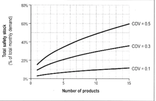
Another key effect of product complexity is its impact on forecast accuracy. As product variety is increased, demand is segmented and the benefit of demand pooling is reduced. As forecast error

increases, the inventory required to maintain a minimum customer service level increases. Perumal demonstrates how both the number of products and variation in demand impact overall safety stock in Figure 4.

Figure 4. Perumal's depiction of total safety stock as a function of product variety for different levels of demand variation

0 I-CIS TP 0_

TI

COV= 0.5

COV= 0.3

-21,r% -1-I

Fr%

_jo

I

15

Number of products

The interactions of product complexity on process complexity and organizational complexity are quite clear. As product variety increases, we see process complexity increase through the breakdown of inflexible processes and the erosion of capacity. Organizational complexity increases as fixed assets are acquired and the cost of administration and holding inventory rises. Low utilization, fixed assets depreciation costs, and large inventories combine to add hidden complexity costs to the organization. In the next chapter, we will discuss how these costs hide in the costing system of Company X

r 40%

-0

COV 0. 1

3

Costing System Analysis

In this chapter, we bring context to this research. Specifically, we discuss the costing system of Company X. This analysis will include an inspection of the costing system, as well as the

implications it has for the SKU rationalization and SKU portfolio management projects.

Another factor relevant to consider is the company's costing system and the transparency of cost across the organization. Standard-costing systems can hide the costs associated with variety.

Many companies spread the cost of setup times, machine downtimes, warehousing & distribution, and overhead across their finished products based on sales volumes. We will quickly review these areas with reference to Company X and the company's vulnerability to hidden complexity costs.

With regard to setup times and down times, Company X has a budget process that includes planned setup and down times at the SKU level. Although, it is not clear that production variances are allocated back to the SKU level once computed. If Company X does not allocate the variances at the SKU level, the effect of SKUs with erratic order frequencies and the impact of production planning on setup times will be hidden.

In the area of warehousing, distribution, and material handling, Company X segments costs in two different ways. Handling costs during the manufacturing or packaging process are allocated by weight. This is more accurate than by sales volumes but does not consider the number of orders

processed for a given product, which is essentially a setup-time that should be accounted for. Warehousing and distribution costs of the finished product are then allocated at the brand level or

charged to the country organization distributing the product. This is another example of costs that can accumulate with variety but are hidden by the costing system.

Overhead costs brought from SKU complexity can also be hidden by Company X's costing system. These costs are spread across the finished product SKUs based on direct costs and equipment costs. This allocation method hides the complexity of low volume SKUs that eat up capacity and warehouse space.

Company X could benefit from some of the latest costing methods but a transformation of this type is outside the scope of this research. We focus on the impact on cash flows and capacity from SKU rationalization and SKU portfolio management.

Along with the hidden complexity costs associated with Company X's costing system, the organization also compartmentalizes cost data from certain stakeholders. Company X's policy

restricts cost data from being shared outside of headquarters. This, of course, has significant implications for SKU rationalization and SKU portfolio management. In order to align marketing and sales stakeholders, a top-down order from upper management must be used or Company X's cost transparency policy must be changed. For this research, both methods were taken to

communicate the benefit of complexity reduction. In 2012, Company X has plans to measure sales management based on both volumes and profitability but at this time the metric is only planned at the brand level. Further, the complexity reduction project is now championed by a sales and finance leader in a key market region.

4

SKU Optimization Process for Healthcare Companies

In this chapter, we devise a data-driven process to optimize a brand's variety offered to the market through SKU rationalization and SKU portfolio dashboards. This SKU process includes:

- A method to identify brands and SKUs for rationalization

- A collection of models to compute the operational and cash flow benefit of rationalization - A dashboard to monitor and sustain the optimum SKU portfolio.

This chapter begins with a description of the SKU Rationalization process along with key metrics and requirements. Following this description, we dive deep into the implementation steps for SKU

rationalization, as well as, details on how to compute the benefits of rationalization. Then, we discuss how dashboards help manage each brand's variety. We conclude with a summary of the benefits of this approach.

4.1

Overview

The SKU optimization process aims to achieve the following objectives:

- Identify SKUs within a brand and/or country that when rationalized will reduce cost and complexity without impacting sales volumes

- Identify the SKU or SKUs within a brand's offering that should not be rationalized due to customer and regulatory requirements

- Compute the quantitative benefit (aka the removed complexity cost) from reducing variety within a brand offering

- Use dashboards to support governance measures and ensure sustainability of optimized brand variety

- Communicate the value and impact of complexity reduction to stakeholders

Each objective was measured through a series of metrics and tools to assess the progress of our research and complexity reduction overall.

4.2

Metrics

In order to measure success, we define the complexity cost as the impact that rationalization of a brand has on cash flows, labor hours, machine hours, forecast accuracy, inventory, number of SKUs per healthcare product, and sales per SKU. We detail each of these metrics below.

Cash flows are defined as "the movement of money into or out of a business, project, or financial product" [4]. The effect on cash flows is more appropriate than the impact on accounting costs because each SKU has different percentages of avoidable and unavoidable costs. This is mostly attributed to different material costs and manufacturing channels. A global assumption on avoidable costs per SKU does not capture the true effect of rationalization.

4.2.2 Labor hours

A reduction in labor hours is related to cash flows. This metric is communicable and intuitive to stakeholders. For example, if enough labor hours could be reduced to remove the 3rd shift at a packaging plant then there is substantial benefit to direct and indirect costs.

4.2.3 Machine hours

Machine hours are the number of hours in which a machine such as a packaging line is used for setup, packaging, or maintenance. This metric can be appropriate for strategic reasons. Specifically, a company might like to keep capacity utilized at a certain percentage or release capacity for launch products.

4.2.4 Forecast accuracy

Forecast accuracy is a very important metric in the healthcare industry due to the high service level requirements and the reputational cost of stock outs. It is also a significant metric because variety directly affects forecast accuracy.

4.2.5 Inventory

Lower inventories will reduce write-offs and holding costs, which will reduce overall COGS making this an important metric to communicate.

4.2.6 Number of SKUs per product per country

Upper management expects the number of SKUs to be reduced through the complexity reduction initiative. Although this metric is not a direct cost benefit, it communicates an intuitive reduction in complexity and coordination, as well as a signal of progress that is necessary for stakeholder alignment. The lowest SKU complexity possible within the scope of this research is one SKU per product per country.

The metric, sales per SKU, is computed by dividing the total sales volume of a brand by the number of SKUs offered for that brand. This is another metric that is appropriate for communicating to sales teams and signals possible cannibalization of sales. Also, as the number of SKUs offered in a brand is reduced, this metric demonstrates a greater contribution from the remaining SKUs offered to the market.

4.3 Requirements

The SKU optimization process has some key requirements that are necessary for stakeholder alignment and implementation success. Details of these requirements are discussed below.

4.3.1 Reproducibility

The process needs to be easily understood and reproducible in order to make the maximum impact. If the process is reproduced across the brands where there is opportunity, a step-change reduction in cost and complexity is possible.

4.3.2 Zero Sales Impact

The rationalization process must consider the impact on sales that reducing variety will have. If there is a possible impact on sales, rationalization should not be performed.

4.3.3 COGS Improvement

Selection of brands and SKUs for rationalization must consider the impact on COGS. For example, a brand that has COGS lower than the average COGS of the brand portfolio weighted by volume may not be a candidate for rationalization.

4.3.4 Communicable Benefit

Since this process affects the whole organization, the impact of rationalization and associated metrics need to be communicable and intuitive. This benefit is realized in the metrics discussed above. Stakeholder alignment is key to the success of this process and sustainmentof its results.

4.4 Implementation Process

The SKU optimization process is a six-step process from brand and SKU identification to monitoring and sustainment. These six steps include:

1) Brand selection - This step involves selecting candidate brands based on each brand's margin, number of SKUs per product, and the brand's position in its product lifecycle. Cross-functional

stakeholders must evaluate and approve selected brands to ensure alignment with the overall company strategy.

2) SKU selection - Within a brand, we segment the SKUs based on market requirements, sales channel, and product. For each, we identify the most common packaging based on sales volume. Finally, we identify candidate SKUs for rationalization within each segment based on volume, demand variation, and margin.

3) Sales impact analysis - In this analysis, we categorize the probability of a significant sales impact for a given SKU if it is rationalized. Each category is based on sales volume and the current finished product offering in a country.

4) Costing system analysis - Before computing complexity cost, we investigate the cost areas that will be affected by SKU rationalization. Further, we identify which of these costs are actually avoidable costs.

5) Complexity cost computation - We apply models of production and forecasting to simulate a rationalization scenario for the brand. The outputs of the models include the effect on cash flows, capacity, inventory, and forecast accuracy. These outputs can be used for the business case to rationalize the selected SKUs.

6) Monitoring and sustainment - In order to sustain the optimum brand variety, the SKU complexity of the brand must be transparent to the organization. We recommend a SKU portfolio dashboard that brings transparency to the creation and removal of SKUs, as well as the metrics described above. If the brand deviates outside the boundaries of an optimal variety, it should be again be considered for SKU rationalization. This dashboard can also be used as governance measure for the creation of SKUs.

We design these steps to formulate a data-driven process for SKU optimization at a healthcare company. 4.4.1 Brand Selection

As mentioned, brands are selected based on margin, number of SKUs, and the brand's position in its product lifecycle. With regard to margin, if a company seeks to improve the overall profitability of its brand portfolio, intuitively brands that are below the average margin of the portfolio might be candidates

for rationalization. Of course, these brands with relatively lower margin need to present an opportunity for SKU rationalization. Only if the brand has a large number of SKUs based on the number of products offered and the number of markets served is the brand actually a candidate for rationalization.

Brands can also be selected for qualitative reasons. These qualitative reasons are based on the current point in the brand's lifecycle. Each stage of the product lifecycle presents opportunities to perform SKU rationalization:

- Launch - Shortly after a brand is launched, rationalization can be performed. One or two years after launch, organizations can review sales volumes of a brand's variety and rationalize the low value SKUs in the market. Further, the brand launch team can avoid unnecessary complexity reduction by launching a lean variety for new products, in which finished product variety is limited.

- In-Market - Another opportunity to rationalize occurs when a brand's production needs to be transferred from one manufacturing site to another site. The cost and risk of transfers can be minimized through rationalization.

e End of Lifecycle - A reduction in a brand's sales volumes and market effects such as

competitor entry present opportunities to rationalize and maximize the profit contributed by the brand. Rationalization of old brands depends on the company's strategy for the brand. If the brand is strategic, rationalization may not make sense. On the other hand, if the brand is not strategic but the company provides the brand for market access, rationalization allows the company to optimize the contribution of the brand.

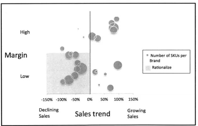
For brand selection, we recommend a cross-section of margin, lifecycle status, and the number of SKUs per brand. Figure 5 demonstrates an example of this cross-section.

Figure 5. Example comparison of margin vs. sales trend over 3 years vs. SKU complexity of brand portfolio

U I

High

Margin

Brand Rationalize

Low

-150% -100% -50% 0% 50% 100% 150%

Declining Growing

In the figure above, we identify a brand as a candidate for rationalization if that brand has a high number of SKUs, declining sales over the last three years, and a low margin relative to the company's portfolio margin. This method presents a way to perform a data-driven decision for brand selection using high-level information. Alternatively, brands can also be selected for qualitative or strategic reasons. Some possible rational for qualitative selection include the following:

- Brands impacted by footprint consolidation - Brands that are no longer core to the business

- Brands affected by external forces such as competition.

With brand selection complete, the next step of SKU selection should begin. 4.4.2 SKU Selection

Given a brand, we select SKUs for rationalization based on sales volume and demand variation within a market segment, as well as opportunities for packaging harmonization. A market segment is defined by market region, sales channel, and product. Each market segment characteristic is defined below:

- Packaging material requirement - Some markets require a specific packaging material for safety purposes. This requirement diminishes packaging standardization.

- Sales channel - _{Healthcare products can be packaged differently depending on the sales channel.}

These channels can include businesses, consumers, or others. Depending on the product, healthcare companies might need to support many of these channels, which increases necessary SKU complexity.

- _{Product version - Many brands have several different product versions. Each version has two} dimensions, which we will not explain for confidentiality purposes.

4.4.3 Identify Market Segments

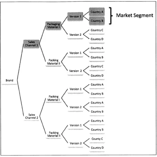
The first step in SKU selection is to identify the market segments within a brand based on sales channel, packaging material requirements, and product versions. Market segments depend on requirements served by the firm and could include more dimensions than these three. Figure 6 below highlights one sales channel within the SKU complexity tree of a brand that has two sales channels, two packaging requirements, and two product versions.

Figure 6. SKU complexity tree with a highlighted market segment

Market Segment

~

P~kirr Verion I

<

C ountry A Verson 2 -,< Country 3

KCountry

In the figure above, the example brand has eight different market segments. Each market

segment has different constraints for rationalization since the sales channel, packaging material

requirement, and versions all impact the requirements of the product's packaging. Next, we identify the priority markets and the most common packaging.

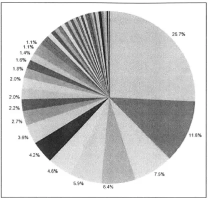
4.4.4 Identify Priority Markets

In order to identify the priority markets, we apply the Pareto principle [5] to determine which

markets account for 80% or more of the sales volume. Markets with high sales volumes can justify SKU complexity if the demand variation is low. This will be discussed further later in this chapter. In Figure

Figure 7. Priority markets identified by pareto principle (Each color represents a different market)

4.4.5 Identify Common Packaging

Next, we identify the most common packaging within a market segment. Our research finds that brands usually have one packaging type that accounts for a majority of sales volumes within a market segment. In these cases, the other packaging types have small volumes unless there is a market requirement for a certain type. This relationship is depicted for one market segment below in Figure 8. Figure 8. Packaging type vs. market segment sales volume of total brand sales

Packaging Type

C

0 2 4 6 8 10 12 14 16 0600% 1.000% 1.00% 2.000% 2.600% 3.000% Number of Records Sum of % of Sales

This view is useful to identify how an variety can be harmonized. In this example, there is an opportunity to rationalize SKUs with packaging type A and B.

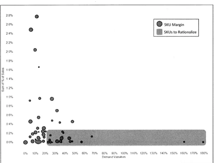
4.4.6 Identify SKUs for Rationalization

With market segments, priority markets, and the most common packaging identified, we have the understanding necessary to correctly determine the opportunity for rationalization. To identify the SKUs

1.1% 1.1% 1.4% 2.0% 2.D% 2.2% 2.7% 11.6%

within each market segment, we look at the sales volume and demand variation of each SKU. As discussed in Chapter 2, SKUs with low volumes and high demand variation bring cost and complexity into an organization. These SKUs are selected for rationalization with two constraints:

- Priority markets -SKUs that serve priority markets can be exceptions to this selection process. - Most common packaging - SKUs that account for the majority of sales volumes within a market

can be exceptions to this selection process.

Leveraging sales data, we develop the following figure to identify the candidate SKUs. Figure 9. Example of SKU selection based on sales volume and demand variation

2r4i SKU Margin

4 SKUs to Rationalize

I %

In the figure above, we highlight SKUs with high demand variation and a low percentage of the sales volumes as candidates for rationalization.

We design this process in order to target SKUs that are redundant and/or cannibalizing sales. Although a sales cannibalization analysis is outside of the scope of this research, we recommend such an analysis if feasible. Instead, we perform a qualitative analysis of the candidate SKUs to assess the risk of a significant sales impact. The SKU selection process targets low volume SKUs so these candidate SKUs will inherently have a low impact on sales. Further, the SKU selection process appropriately selects within market segments. Therefore, we select candidates from a group of SKUs serving the same market and likely meeting the same requirements. Sales transfer is more likely if sales are moved between SKUs that meet similar requirements. As shown in Table 1, we recommend clustering candidates as low, medium, or high risk of sales impact according to certain characteristics, assuming selection within a market segment. Clustering candidates SKUs is important when pursuing management approval. For example, management will allow approve rationalization of low and medium risk SKUs but not high risk. Table 1. Risk assessment of sales impact

Risk Sales Channel Packaging Type Volume

Low Free goods / General Redundant / Unique < 1% of sales Market

Medium General Market Unique 1-2% of sales

High Priority Customer / Unique > 2% of sales

Market Requirements

The complexity reduction team should aggressively pursue rationalization of free goods,

redundant, and/or low volume offerings. Medium-risk SKUs require strong alignment with the marketing and sales teams of the respective market to confirm feasibility. These SKUs have a unique pack size or packaging and 1-2% of sales. And finally, high-risk SKUs account for large sale volumes or might meet a specific market requirements. We recommend that the organization strongly consider the context of their customers and markets when assessing the risk of sales impact.

4.4.8 Costing System Analysis

As discussed in Chapter 2, complexity costs refer to costs that are difficult to quantify using common organizational costing systems. Although costing systems will not itemize the complexity costs, we perform a thorough analysis to achieve an understanding of where costs will be reduced due to SKU rationalization. Some of these cost reductions are intuitive such as the reduction in labor costs due to less setup times on a packaging line. Other cost reductions are second order effects such as avoidance in

capital investment to increase capacity or reduced costs to transfer production between manufacturing sites. We focus this analysis on costs that are directly affected by SKU rationalization.

To begin, we work with company stakeholders who know the cost accounting system from the plant to the global aggregated costs in order to understand each major itemized cost in their costing system. If the brand is sourced from multiple locations or value chains, the cost allocation differences must be understood between each channel.

With an understanding of these costs, we generate a table of the itemized costs and how these costs are affected by SKU rationalization and whether the costs are avoidable and should be quantified. An example is shown in Table 2.

Table 2. Example of an organization's itemized costs

Cost Item Includes Effect of SKU Avoidable Quantify?

Rationalization

Raw Material - Non-packaging Possible volume Partial No. Now-packaging

Costs Raw Materials discounts from raw materials

- Packaging packaging accounts for majority

Materials harmonization of cost but are

unaffected.

Direct Labor - Setup time Removal of setup Partial Yes. Setup times can

- Processing time times be greater than

- Maintenance processing and

maintenance times. Fixed Assets - Utilization Frees capacity hours No, unless Yes. Quantify freed

- Depreciation from less setup times removal of capacity to avoid

- Leasing high capital investment.

number of No direct cash flow SKUs effect.

causes divestment of fixed asset

General - Management Less coordination No No

Overhead 0 Support

Utilities - Electricity Possible reduced Partial No. Small

- Heating/Cooling labor shifts percentage of total

cost.

Warehousing Shipping and Reduced order Yes Associated labor is

& Distribution handling processing avoidable and

labor

This step is important because it allows the complexity reduction team to understand where the value of SKU rationalization is coming from and to focus on cost areas to quantify. In the next section, we will quantify the affected cost areas.

4.4.9 Complexity Costs Calculation

With SKUs selected for rationalization and an understanding of cost allocations within the organization, we compute the complexity cost associated with the current brand variety. We define complexity cost as the sum of the impact that increased SKU variety has on cash flows, inventory, and avoidable costs. This relationship is demonstrated in Figure 10 below.

Figure 10. Definition of complexity costs

We discuss each complexity cost element and its calculation in detail below. In brief, we

compute the impact on cash flows by modeling the current and future state of setup times and labor hours on production lines. Next, we calculate the impact on inventory holding costs by modeling the current and future state of cycle stock and safety stock inventory levels.

4.4.9.1 Production Model Formulation

The purpose of the production models is to quantify the reduction in labor hours, the impact on utilization, and the effect on replenishment time that SKU rationalization has on operations. We create two models to capture the impact on operations - a descriptive model and a queuing model. The

descriptive model uses historical data and highlights the reduction in setup time if SKU rationalization is

performed. The queuing model captures the effect on utilization and replenishment time from SKU rationalization.

4.4.9.1.1. Descriptive Model with Economic Order Quantity

The descriptive model is a scenario analysis that quantifies how much non-value added time could be reduced if a lean variety was offered for a given brand. We focus on the packaging process in this model for the following reasons:

- Production quantities of healthcare product raw materials are computed by pooling demand of each SKU and therefore are not strongly impacted by SKU variety.

- Rationalization of healthcare versions are outside of the scope of SKU rationalization

- The scope of SKU rationalization focuses on finished product SKUs and driving efficiencies in the packaging process step

Further, we focus on cash flows in order to compute a quantifiable benefit that is separate from a debate regarding accounting costs. This allows us to capture a benefit that is easily communicable to external stakeholders. In this section, we discuss the inputs, outputs, calculations, and assumptions associated with this model.

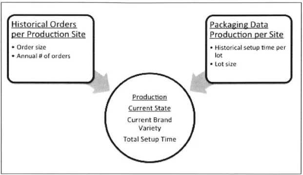
4.4.9.12 Inputs and Assumptions

In order to determine the current state of total setup time for the brand, the model requires the following historical information for each SKU:

- Annual number of orders - Order quantity per order - Production lot size - Setup time per lot

Figure 11. Current state of production model

Historical Orders

Packaging Data

per Production Site

Production per Site

* Order size * Historical setup time per

+ Annual # of orders lot

Lot size

Production Current State Current Brand

Variety

Total Setup Time

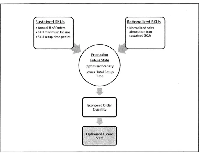
To compute the future state of total setup time, the model requires the new lean product offering and its associated volumes. The remaining SKUs that are not rationalized make up the lean offering. The sales volumes of the lean product variety are the sum of current volumes of sustained SKUs and the volumes of rationalized SKUs that are transferred to sustained SKUs, assuming zero sales impact.

Initially, we assume in the future state that the number of orders per year of each SKU stays constant. We then relax these constraints and include the benefits of computing the economic order quantity for each sustained SKU. The process behind capturing the future state is depicted in Figure 12 below.

Figure 12. Future state of production model

Sustained SKUs * Annual # of Orders * SKU maximum lot size * SKU setup time per lot

Rationalized SKUs * Normalized sales absorption into sustained SKUs Production Future State Optimized Variety

Lower Total Setup Time Economic Order Quantity Optimited Future Ste 4.4.9.1.3 Outputs

The outputs of this model match up with many of the metrics described earlier in this chapter. These metrics include the following:

- Cash flows - Labor hours

For each metric, we compare the current and future state to determine the benefit of the future state. 4.4.9.1.4 Model Formulation

The computation for this model is trivial which makes the process reproducible and the benefit easily communicable. Both characteristics are requirements of the model. Further, the model has two computations, which include:

- Economic order quantity

4.4.9.1.4.1 Total Setup Time

To compute the total setup time annually for a given brand, we employ the parameters detailed in Table 3.

Table 3. Parameters of total setup time equation

Lot size of SKU i Packaging Units

s, Setup time per lot of SKU i Hours

qj Order quantity of orderj of SKU i Packaging Units

Using these parameters, total setup time is computed as follows: Equation 1. Total setup time for n SKUs of a brand

=517 Sj

This equation is used to compute the total setup time of both the current variety and the future lean offering. The reduction in setup hours is equal to reduction in labor hours required to meet demand. The effect on cash flows is simply computed by multiplying the number of heads per shift by the number of setup hours reduced.

4.4.9. 1.4.2 Economic Order Quantity

For each sustained SKU, we recommend applying the economic order quantity (EOQ) model to determine the optimal lot size to produce that minimizes setup costs and holding costs. The parameters for the EOQ model are detailed in Table 4.

Table 4. Parameters of economic order quantity model

Cost of setup $/order

Ii

A

D Annual demand items

r Holding cost $/$/year

Using these parameters, the economic order quantity is computed as follows: Equation 2. Economic order quantity 181

2AD EOQ =

vr

4.4.9.15 Summary

With this model, we determine the complexity cost associated with the cost of setup time for the current offering sold to the market in comparison to the setup time cost of a lean offering. By quantifying labor hours, this model meets the requirement that the benefit of SKU rationalization can be easily be communicated to stakeholders. Further, this model maps SKU complexity to operational complexity. Although the model only captures the effects on labor hours, this output could provide the impetus for fixed cost reduction such as capital investment avoidance, a work shift reduction, or footprint

consolidation.

4.4.9.2 Queuing Model [6]

The queuing model allows us to analyze the impact of SKU complexity on capacity, utilization and replenishment time. For the queuing model, we use the simple M/M/l system. In the case of packaging, we did not assume that any available packaging line could service an order. Instead, we analyze each packaging line and its associated demand using the M/M/l system to determine the overall impact on utilization and replenishment time. With a M/M/1 system, both the arrival process and service process are memory-less and there is one server or packaging line in the system.

SKU complexity impacts both the arrival process and service process by increasing the number of

orders and the utilization time. With constant demand, an increase in orders leads to an increase in arrival rates and a reduction of service time due to setups. To understand the impact of SKU complexity, we compare the queuing system with the current product variety to the queuing system with a lean offering.

4.4.9.2.1 Inputs and Assumptions

The queuing model requires information regarding the arrival process, the service process, and the available processing time. Regarding the arrival process, we assume a Poisson process. The input of the arrival process is the annual orders per year processed by the packaging line and the available hours for receipt of orders. The available hours are the number of hours in a year that the packaging line is operating and ready to setup for or to process an order.

The input of the service process is the number of orders received annually, the number of units produced annually, the total setup time to produce the aforementioned volume, and the service rate of the packaging line. Packaging lines rates can be in terms of units per minute.

4.4.9.2.2 Outputs

The queuing model provides the following expected values of the performance of the system [6]: * Total runtime - _{the theoretical total time that the packaging line is producing units per year}

* Total setup time - the theoretical total time that the packaging line is being setup to produce per year

* Utilization - the percentage of time that the packaging line is in use for processing over the course of the year

- Expected waiting time - the expected number of hours an order will need to wait before being processed

- Expected queue length - the expected number of orders waiting to be packaged - Expected system time - the expected time for an order to be processed

* Expected number in system - the expected number of orders in the system (i.e. orders are either in the queue or being processed by the server)

4.4.9.2.3 Model Formulation

The queuing model is a standard M/M/l system and applies the following equations as defined by the model to approximate the outputs mentioned above.

Equation 3. Expected # of orders in system 161

L=

(1- p)

Equation 4. Expected system time of an order 161 W =

a(1 -p)

Equation 5. Expected length of the queue 161

pz

Q

P

Equation 6. Expected queuing time of an order 161

p2 D =

A(1 - p)

p uapacity utilization Percent

A

A depiction of the M/M/1 queing model is shown in Figure 13 below.

Figure 13. M/M/1 queuing model [61

System

Sevc

Orders

arive

Finished

(Arrival

~

Products

rate X)

exit

The queuing model captures the effects of SKU complexity on replenishment lead-time and cycle stock. A change in SKU complexity impacts both setup time and the arrival rate in the queuing system.

If the SKU complexity is reduced, we observe a decrease in replenishment lead-time. Lower lead-times

contribute to improved forecast accuracy and decreased cycle and safety stock.

For computation of the associated complexity cost element, we use the difference between the expected system time of the current and of the future state. This lead-time reduction is used to quantify a savings in both cycle stock and safety stock.

4.4.9.3 Forecast Accuracy Model

We formulate a forecasting model to quantify the improvements in forecast accuracy that are possible through the demand pooling that occurs with the implementation of SKU rationalization. By improving forecast accuracy, the company can reduce safety stock and write-offs, and therefore, complexity costs. We measure forecast accuracy as the Mean Absolute Deviation (MAD) divided by

average sales and use the standard calculation for safety stock. In this section, we discuss our assumptions, the inputs and outputs of the model, the model's formulation, and the benefits of this analysis.

4.4.9.3.1 Input & Assumptions

In order to compute the MAD/Mean ratio, we collect at least one year of historical forecasting data for the brand selected for SKU rationalization. This data includes the forecast for demand over the lead-time period and the actual demand over the lead-time. The forecast accuracy for the current brand variety can be computed with this data.

For the future state, the candidate SKUs for rationalization and the SKUs that will absorb the sales of these rationalized SKUs are required. By combining demand, we leverage the benefits of risk pooling in reducing forecast error. The two inputs of the future state model are the sum of forecasted demand and the sum actual demand for each collection of pooled SKUs.

4.4.9.3.2 Outputs

The output of the model is the improvement in forecast accuracy in terms of percentage points. The output is provided in improvement by affected SKUs but can easily be computed for other contexts including the following:

- Improvement by brand

- Improvement by market packaging requirements - Improvement by sales channel

- Improvement by country - Improvement by product version 4,4.9.3.3 Model Foimulation

Both the current state formulation and future state formulation use the MAD/Mean ratio. The MAD or mean absolute deviation is the absolute average difference between the forecasted demand and

actual demand [7]. The Mean is the average demand over the measurement period. We recommend the use of at least one year of measurement. The formulation for the MAD/Mean ratio is as shown in Equation 7.

Equation 7. Formulation of MAD/Mean ratio 171

1=illi -

ail

n n

where,

e n -the number of periods of measurement (i.e. weeks, months, years)

Sfi

In the future state, the variables represent pooled forecasted demand and pooled actual demand. In other words, the sales volumes are transferred from a rationalized SKU to a sustained SKU as shown in Table

5.

Table 5. Representation of demand transfer from rationalized SKU to sustained SKU

SKU Number Current Demand Future Demand SKU Future Status

1 X 0 Rationalized

2 Y X normalized + Y Sustained

The improvement in forecast accuracy is simply computed as the difference between the current and future state forecast error. Improved forecast accuracy will reduce write-offs, lost sales, and safety stock, all of which are complexity costs driven by SKU complexity.

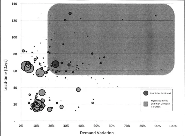
Safety stock is further reduced due to a correlation that we find between high demand variation and long times [18]. This can be investigated by simply comparing demand variation versus lead-time as shown in Figure 14. In this figure, we see that low volume SKUs (shown by small bubbles) exist to the top right of the graph. This shows that the SKUs in the red region will have a larger effect on safety stock reduction if replaced by SKUs in the non-red regions.

Figure 14. Demand variation vs. lead-time vs. % of brand sales per SKU 140 120 100 80 60 C0 E -0

~J

For rationalized SKUs that are replaced with SKUs that have shorter lead-times, we can compute a multiplicative reduction effect due to the reduction in lead-time and the reduction in forecast error. We compute the complexity costs associated with safety stock by computing the difference in safety stock

levels between the current and future state. This delta is a reduction in holding cost for the brand. We compute safety stock levels using the safety stock equation and historical lead-times as shown in Equation

8.

Equation 8. Safety stock equation for a SKU 191

safety stock = ss = ZoLTD\/T

where,

- z - safety factor for the appropriate service level

- oLTD -standard deviation of forecast over lead-time - LT -order lead-time of a given SKU

We then compute the associated complexity cost as shown in Equation 9. Equation 9. Safety Stock Complexity Cost per SKU

complexity costss = vr(sscurrent - ssfuture)

where,

e v - value per unit of safety stock in $

- r - holding cost in $/$/year

- ss, - number of units of safety stock in period i

4.4.9.3.4 Summary

The forecasting model quantifies how SKU complexity contributes to rising inventory and forecast error. As the number of SKUs increase for a given brand within a sales channel, demand is segmented and forecast error increases. Forecast error has a major impact within the healthcare industry where there are lives in need of these healthcare products. Further, this error is directly proportional to safety stock levels. We also find that high demand variation correlates with longer lead-times. By rationalizing high variation SKUs, SKUs with long lead-times are also removed. This highlights another complexity costs brought by a stronger increase of safety stock due the multiplication of forecast error and the square root of lead-time. As inventory increases, write-offs and working capital increase which further grow complexity costs.

4.4.10 Monitoring and Sustainment

In support of our research, we develop dashboard views of the SKU portfolio to facilitate both the rationalization process, monitor the impact on sales, and to govern SKU creation. In this section, we describe the different views of the dashboard and how these views will benefit the organization.

4.4.10.1 Dashboard Views

Dashboards can be implemented using a variety of IT tools. We recommend using simple-to-use visualization software that can connect real-time to the databases of your organization. Leveraging the IT databases that exist to generate the views that will bring transparency and communicate well to

stakeholders allows you to frame the argument for rationalization, as well as identify the opportunity. For this research, we implement dashboards using Tableau Software. Our dashboards highlight the metrics outlined earlier in this chapter and help identify opportunities for optimizing the SKU portfolio.

Through a dashboard, we are able to quickly bring transparency to key decision criteria for SKU rationalization and to identify good and bad complexity. The views we generate allows us to perform the following:

- _{Identify the emergent most commonly-used packaging for each brand, product version and/or} market

- Compare volumes across product versions - Identify priority markets by brand

- Identify candidate SKUs for rationalization based on SKU complexity, volumes, and priority markets

* Monitor SKU creation trends versus sales trends - Monitor progress of complexity reduction projects

For each capability, we discuss the derived benefit of this transparency. 4.4.10.1.1 Packaging Commonality

One approach to SKU rationalization is to harmonize the variety through common packaging. Due to aspects of the healthcare industry, we find that one packaging type accounts for a majority of the SKU offerings and of a brand's sales volumes. This begs the question of why should the organization support the other packaging types. In Figure 15, we present a view of the packaging offerings within five market segments.

Figure 15. Packaging types for each market segment

Channel Material Version Packaging Type Count.

Gneral 1111 A Market4 D 30 E 2 F 7 G 8 H 1 L 1 2 B 10 D 38 E 2 F 7 8 H1 L I M% 1%3 %5%6 %8 %1% 1 2 3 4 0 80 O2 IM& F% of Tota Ne..Sales Li

Table 6. Explanation of fields in packaging types dashboard

Field Description

Channel Sales Channel (i.e. general market, business,

free goods)

Material Packaging material to meet market

requirements

Version Product version

Packaging Type Type of packaging configuration

Count Number of SKUs of packaging format in

market segment

% of total net sales Percentage of global sales for that brand