HAL Id: hal-02572317
https://hal.archives-ouvertes.fr/hal-02572317
Submitted on 13 May 2020
HAL is a multi-disciplinary open access archive for the deposit and dissemination of sci-entific research documents, whether they are pub-lished or not. The documents may come from teaching and research institutions in France or abroad, or from public or private research centers.
L’archive ouverte pluridisciplinaire HAL, est destinée au dépôt et à la diffusion de documents scientifiques de niveau recherche, publiés ou non, émanant des établissements d’enseignement et de recherche français ou étrangers, des laboratoires publics ou privés.
J. Coston-Guarini, J.-M. Guarini, Shawn Hinz, Jeff Wilson, Laurent Chauvaud
To cite this version:
J. Coston-Guarini, J.-M. Guarini, Shawn Hinz, Jeff Wilson, Laurent Chauvaud. A roadmap for a quantitative ecosystem-based environmental impact assessment. ICES Journal of Marine Science, Oxford University Press (OUP), 2017, 74 (7), pp.2012-2023. �10.1093/icesjms/fsx015�. �hal-02572317�
TITLE 1
A roadmap for a quantitative ecosystem-based environmental impact assessment 2
3
SUBMITTED TO: 4
ICES Journal of Marine Science “Special MSEAS-2016 issue” 5 as an ORIGINAL ARTICLE 6 7 AUTHORS 8 J. Coston-Guarini1,2,3 9 [email protected] 10 11 J-M Guarini1,3 12 [email protected] 13 14 J. Edmunds4 15 [email protected] 16 17 Shawn Hinz5 18 [email protected] 19 20 Jeff Wilson5 21 [email protected] 22 23 L. Chauvaud3,6 24 [email protected] 25 26 AFFILIATIONS 27
1 The Entangled Bank Laboratory, Banyuls-sur-Mer, 66650 France
2 Ecole Doctorale des Sciences de la Mer, UBO, CNRS, UMR 6539-LEMAR IUEM
29
Rue Dumont d’Urville Plouzané, 29280 France 30
3 Laboratoire International Associé ‘BeBEST’, UBO, Rue Dumont d’Urville Plouzané,
31
29280 France 32
4 LimOce Environmental Consulting, Ltd. 47 Hamilton Sq. Birkenhead, CH41 5AR UK
33
5 Gravity Environmental Consulting, Fall City, WA, 98024 USA
34
6 CNRS, UMR 6539-LEMAR IUEM Rue Dumont d’Urville Plouzané, 29280 France
35 36 CORRESPONDING AUTHOR 37 Jennifer Coston-Guarini 38 39 Mailing address: 40
Ecole Doctorale des Sciences de la Mer, UMR 6539-LEMAR, 41
IUEM 42
Rue Dumont d’Urville Plouzané, 29280 France 43 44 45 46 VERSION 47 1 Sept 2016 48 49
ABSTRACT 50
A new roadmap for quantitative methodologies of Environmental Impact Assessment 51
(EIA) is proposed, using an ecosystem-based approach. EIA recommendations are 52
currently based on case-by-case rankings, distant from statistical methodologies, and 53
based on ecological ideas that lack proof of generality or predictive capacities. These 54
qualitative approaches ignore process dynamics, scales of variations and 55
interdependencies and are unable to address societal demands to link socio-economic 56
and ecological processes (e.g. population dynamics). We propose to re-focus EIA 57
around the systemic formulation of interactions between organisms (organized in 58
populations and communities) and their environments but inserted within a strict 59
statistical framework. A systemic formulation allows scenarios to be built that simulate 60
impacts on chosen receptors. To illustrate the approach, we design a minimum 61
ecosystem model that demonstrates non-trivial effects and complex responses to 62
environmental changes. We suggest further that an Ecosystem-Based EIA - in which the 63
socio-economic system is an evolving driver of the ecological one - is more promising 64
than a socio-economic-ecological system where all variables are treated as equal. This 65
refocuses the debate on cause-and-effect, processes, identification of essential portable 66
variables, and a potential for quantitative comparisons between projects, which is 67
important in cumulative effects determinations. 68
69
KEYWORDS 70
Environmental Impact Assessment, ecosystem, drivers of change, modelling, socio-71
ecological system 72
INTRODUCTION 74
When the USGS hydrologist and geomorphologist Luna Leopold (1915-2006) and his 75
two co-authors published a system for environmental assessment in 1971 (Leopold et 76
al., 1971), they could not have foreseen that 50 years later, their report would be at the 77
origin of a global industry (Morgan, 2012; Pope et al., 2013). Leopold et al. produced 78
their brief document at the request of the US Department of the Interior after the 79
National Environmental Policy Act (NEPA) created a legal obligation for federally 80
funded projects to assess impact. In the year following the passage into law, the 81
scientific community was quick to point out the absence of any accepted protocol for 82
either the content of the document or its evaluation (see characterisation in Gillette, 83
1971). In response, Leopold et al. describes a preliminary approach, with a simple 84
decision-tree like diagram (Figure 1A) relying on structured information tables. These 85
tables of variables and qualities, or ‘interaction matrices’, are intended to enforce 86
production of uniform, comparable descriptions, while requiring only a minimum of 87
technical knowledge from the user. 88
Impact inference rests on a statistical comparison of variables between impacted and 89
non-impacted sites, but assessing an impact is understood to include value-based 90
judgements about quality and importance (Leopold et al., 1971) linked with attitudes 91
held about the environment (Buttel and Flinn, 1976; Lawrence, 1997; Toro et al., 2013). 92
These judgements, often made a priori (Toro et al., 2013), can conflict with the 93
necessity to reach a legal standard of proof (Goodstein, 2011) when projects are 94
contested. EIAs therefore embody a compromise between technical descriptions of the 95
expected magnitude of an impact on a receptor and managerial recommendations about 96
how to avoid that receptors exceed acceptable values, or mitigate, identified impacts 97
(Lawrence, 1997; Cashmore et al., 2010; Barker and Jones, 2013). By 1971, under 98
pressure to move development projects forward (Gillette, 1971), the EIA process 99
became institutionalised as a qualitative exercise focussed on collecting documentation 100
about a project site supported by individuals’ professional expertise, without requiring 101
quantitative evaluations to back up statements (Lawrence, 1997; Cashmore et al., 2010; 102
Morgan, 2012; Toro et al., 2013). Hence EIAs today still strongly resemble the 103
preliminary instructions given by Leopold et al. (Figure 1B). Consequently, review 104
articles, such as that of Barker and Jones (2013) on offshore EIAs in the UK, often 105
report strong criticisms of the quality of environmental impact documents as being 106
“driven by compliance rather than best practice”. 107
Over the past decade, technologically sophisticated monitoring tools and baseline 108
surveys have been integrated (e.g. Figure 1B, “Modelling”; Payraudeau and van der 109
Werf, 2005; Nouri et al., 2009) on a discretionary basis because they contribute to risk 110
management of sensitive receptors as well as to new dynamic features like the “Life 111
Cycle Assessment” of a project (Židonienė and Kruopienė, 2015). These changes 112
suggest that EIA is poised to incorporate quantitative frameworks. 113
Inspired by the application of ecosystem-based management frameworks in fisheries 114
(Smith et al., 2007; Jacobsen et al., 2016), and by the generalisation of modelling and 115
statistical tools in ecological and environmental sciences, we describe in this article how 116
the objective of a quantitative, ecosystem-based EIA could be achieved. We first 117
examine briefly the awareness of impact and analytical approaches that exist to quantify 118
this within ecological sciences. We then propose a quantitative reference framework 119
linking statistical impact assessment to ecosystem functioning and discuss how the 120
modelling approach may be used to provide reasonable predictions of different 121
categories of impact. Finally, we explore how our ecological system will behave when 122
socio-economic “drivers of change” (UNEP, 2005) are implemented. By imposing 123
socio-economic factors as drivers (instead of as variables of a large integrated system), 124
we show that different types of consequences can occur, which are not represented by 125
classical feedbacks. For example, this permits the life cycle of the project to be 126
described as a driver of the dynamic of the impacted system, or the explicit 127
implementation of cumulative effects scenarios. 128
Awareness of environmental impact in the past. There is a long written record of the
129
awareness that human activities affect the environment. Texts of 19th century naturalists
130
commonly contain remarks about the disappearance of animals and plants attributed to 131
human activities; some are quite detailed, like George P. Marsh’s quasi-catalogue of the 132
ways “physical geography” (natural environments) has been altered by development 133
(Marsh, 1865). Most are ancillary comments to make rhetorical points, rather than 134
scientific observations, like this quote from the marine zoologist Henri de Lacaze-135
Duthiers (1821-1901) (de Lacaze-Duthiers, 1881: 576-577): 136
“Ainsi, lorsque sera crée la nouvelle darse, qui n'a d'autre but que d'augmenter le 137
mouvement du port, que deviendront les localités tranquilles où la faune était si riche ? 138
Resteront-elles les mêmes ? l’eau ne se renouvelant pas, n'aura-t-elle pas le triste sort 139
de celle des ports de Marseille, si le commerce et les arrivages prennent de grandes 140
proportions ? 141
“Le mouvement du port augmente tous les jours. Les constructions des darses projetées 142
ne modifieront-elles pas les conditions favorables actuelles ? On doit se demander 143
encore si l'eau conservera son admirable pureté quand le nombre des bâtiments aura 144
augmenté dans les proportions considérables que tout fait prévoir. 145
“Port-Vendres ne peut évidemment que se modifier profondément dans l’avenir, et cela 146
tout à l’avantage du commerce, c’est-à-dire au détriment de la pureté, de la tranquillité 147
de l’eau et du développement des animaux. 148
A Banyuls, il n’y a aucune crainte à avoir de ce côté.” 149
When he wrote this, Lacaze-Duthiers had been lobbying for more than a decade for the 150
creation of a network of marine stations in France. His text justifies why he chose a 151
village without a port, instead of one with a thriving port. His reasoning is that 152
economic development causes increases in buildings, docks, boat traffic, that damages 153
the “tranquillity”, “water purity”, and the “favourable conditions for development of 154
fauna”. While he acknowledges this is a gain for local commercial interests, it is also at 155
the expense of faunal richness, and he predicts this will lead to the “sad situation of the 156
port of Marseille”. Lacaze-Duthiers feels this degradation should be a legal issue or a 157
civil responsibility (as “au détriment de” indicates a legal context). The attitude and 158
awareness of Lacaze-Duthiers are symptomatic of ambiguities about the environment 159
(Nature) and the place of humans in it, that are also at the core of EIA (Cashmore, 2004; 160
Wood, 2008; Morgan, 2012; Toro et al., 2012). These political conflicts between a 161
desire to preserve the natural world and its own functioning, and the desire to use, 162
exploit, order and control parts of it are the main issues of impact assessment 163
(Cashmore et al., 2010). 164
Path to reconciliation. What changed in the latter half of the 20th century is that
165
managers, regulators and stakeholders need to document and quantify impacts as well as 166
their associated costs. However, important, historical contingencies complicated the 167
development of quantitative tools for environmental impact. Ecosystem science, which 168
pre-dates EIA by several decades, describes ecosystem functioning in terms of energy 169
and mass flows (e.g. Odum, 1957) and the distribution of species is understood with 170
respect to how well the ‘conditions of existence’ of a population are met and maintained 171
(e.g. Gause, 1934; Ryabov and Blasius, 2011; Adler et al., 2013). These approaches use 172
paradigms from biology, physics and chemistry to describe functions and quantify 173
fluxes. Consequently, ecosystem science was not concerned with characterising 174
environmental quality, but determining when conditions of existence were met within 175
dynamic, interacting systems. By the 1970s when EIA practice emerged, ecological 176
research was busy with adaptation and community succession (Odum, 1969; McIntosh, 177
1985), while the concepts of environmental quality and impact were being defined 178
under a “political imperative, not a scientific background” (Cashmore, 2004: 404) using 179
static components like receptors and indices. 180
Today, several very different, co-existing strategies exist with regards to environmental 181
management and conservation: ecosystem functioning (e.g. Moreno-Mateos et al., 182
2012; Peterson et al., 2009), ecosystem services and markets analysis (e.g. Beaumont et 183
al., 2008; Gómez-Baggethun et al., 2010), and environmental impact. In this context, 184
knitting together sociological and ecological frameworks has emerged as a very active 185
area of interdisciplinary research (Binder et al., 2013). An important theme has been to 186
re-conceptualise environmental dynamics from an anthropogenic perspective to counter 187
a perception that human activities have been excluded from ecological studies (Berkes 188
and Folke, 1998; Tzanopoulos et al., 2013). While this is clearly an unfair 189
characterization (the classic introductory American text on ecology is entitled “Ecology: 190
The link between the natural the social sciences”; Odum, 1975), we do recognize that, 191
historically, ecological sciences have often ignored human behaviours and attitudes in 192
ecosystem studies, despite numerous appeals (Odum, 1977; McIntosh, 1985; Berkes 193
and Folke, 1998). Inspired by the criticisms of Lawrence (1997) about EIA and the 194
challenge of working between both sociological and ecological systems (Rissman and 195
Gillon, 2016), we propose a quantitative basis for systems-based impact assessment. 196
Our goal is to renew the understanding of impact in terms of the interactions and 197
functions attributable to ecosystem processes, integrating the full dynamics of physical 198
and biological processes, while allowing for effective evaluation of socio-economic 199
dynamic alternatives within the modelling framework. 200
201
METHODOLOGY 202
Receptors. Assuming that the screening process has already demonstrated the
203
requirement to perform an EIA for a given project, scoping identifies the receptors and 204
the spatio-temporal scale of the study. Receptors are represented by variables being 205
impacted by the project implementation. Receptors are determined by the experts in 206
charge of the EIA. Their qualifications as receptors imply that they will be impacted and 207
this cannot be questionable. In other words, what is called "testing" impact is 208
statistically limited to a process of deciding if the observation data corresponding to 209
samples of the receptor variables permits an impact to be detected. In no case should the 210
selection of a receptor be made with the objective to decide if there is an impact or not. 211
By definition, receptors are selected because they are sensitive to the impact. However, 212
all declared receptor variables also represent objects of ecology and can be inserted into 213
an ecosystem framework. These two points will now be reviewed in more detail, 214
establishing an explicit link between them. 215
Statistical rationale for impact assessment detection. Impact assessment relies on
216
statistical comparisons of receptor variables in impacted and non-impacted situations. 217
Assuming that the expertise determined the nature of the impact (i.e. decreasing or 218
increasing the variable), the impact assessment consists of testing if the absolute 219
difference, D, between the non-impacted (µ0) and the impacted variable means (µI) is
220
greater than zero (H1: D = |µ0-µI| > 0). Classical testing procedure leads not to accepting
221
H1, but to rejecting H0 (H0: D = |µ0-µI|= 0). However, the power of the test increases
222
when D increases, which means that the more the variable is sensitive, the greater the 223
impact has a chance to be detected. 224
Ideally, as EIAs start before the project implementation, samples of receptor variables 225
are collected before and, then after the project. We focused on this case even if 226
sampling may also be carried out concurrently for comparing non-impacted and 227
impacted zones. For a receptor variable x, considering two samples of sizes n0 (before
228
implementation) and nI (after implementation), the empirical averages are x and 0 xI,
229
respectively, and their standard deviations are s0 and sI. The statistics of the test is then:
230 1 1 0 0 0 -- + -= I I n n s x x y [Eq. 1] 231
emphasizing the importance of the sample (before implementation), which is used to 232
estimate the ‘baseline’. The dispersion around the average s0 has a crucial role in the
233
calculation of y (y decreases when s0 increases). Besides the size n0 will be fixed when
234
the project is implemented (i.e. it is impossible to come back to the non-impacted 235
situation when the project is implemented), while nI can be determined and even
236
modified a posteriori. 237
Under H1 (hence when H0 is rejected), y is normally distributed, y ~ N(D,1), and then it
238
can be centred using: 239
1 1 0 0 0 -- + D -= I I n n s x x y [Eq. 2] 240
This allows us to state that y follows a Student law. Therefore the test leads to rejection 241
of H0 if y is greater than a threshold tu,a, where u is the number of degrees of freedom
242
(u = n0-1) and a, the type 1 error (rejecting H0 when H0 is true), is a = proba{y> tu,a |
243
D=0}). The type 2 error (failing to reject H0 when H0 is false) is then b = proba{y> tu,a |
244
D>0} and the power of the text is p=1-b. 245
As y follows a Student law: 246 b u a u b u 1 1 , 0 0 , 1 , t n n s t t I -= + D -= -- [Eq. 3] 247
Considering that the baseline is estimated by a sampling performed before 248
implementation, with n0 becoming a fixed parameter, the question of detecting
249
significantly the impact then consists of determining two unknown variables D and nI by
250
solving two functions: 251
(
)
(
)
î í ì D = = D b a b a , , , , g n n f I I [Eq. 4] 252By introducing d=D/µ0, the variation D relative to the baseline, and C0=s0/x , the 0 253
variation coefficient of the baseline sample, the system to solve is then: 254
(
)
(
)
(
)
ï ï î ïï í ì + -+ = + + = - -2 , , 2 0 2 0 2 , , 2 0 0 1 1 0 0 , , b u a u b u a u b u a u d d t t C n t t C n n n n C t t I I [Eq. 5] 255At this point in our development, we can make several remarks about how EIA 256
practices shape the calculation of the impact: 257
1. The change relative to the baseline (d) is positive if d >C0
(
tu,a +tu,b)
n0 , and 258 hence * C0(
t , t ,)
n0 b u a ud = + is the detection limit of the receptor variable which 259
can be calculated a priori (before impact). d* is the smallest absolute relative
260
difference that can be characterized, and it depends only on s0 and n0 and the
261
choice of Type 1 and 2 errors. Therefore, the quality of the expertise, which 262
determines the receptors and the baseline, is a fundamental component of impact 263
assessment. 264
2. The parametric framework has many constraints (i.e. homogeneity and stability 265
of the variance, stability of the baseline ...), which have to be ensured, but is very 266
useful for establishing a link with modelling. In particular, µ0 and µI, hence D and
267
d, are descriptors of the states of the impacted ecosystem which can be simulated 268
by calculation from a deterministic model. 269
3. A fortiori, the change relative to the baseline, d, which depends on the nature of 270
the impact and the temporal scale of the observations, can be determined a priori 271
(or plausibly predicted) by the deterministic model. However it implies assuming 272
that the variations which create the dispersion around the trend of the variable are 273
white noises, et (defined by {E(et) = 0, E(et²) = s0, E(eti,etj) = 0}. In this case, the
274
design of the ecosystem becomes particularly important, not only for diagnosing 275
the amplitude of the impact, but also the exact condition of the survey (i.e. 276
calculation of nI).
Building an ecosystem model with receptors. Our means to reconcile impact
278
assessment with the theory of ecology is to replace the notion of receptors into a 279
dynamic ecological model (Figure 2A). Receptors are placed in a network of 280
interactions which represent an ecosystem. The “ecosystem” is a system in which the 281
living components will find all conditions for their co-existence in the biotope (abiotic 282
components and interactions that living organisms develop between themselves and 283
with their environment). This classical definition (Tansley, 1935) encounters problems 284
when translated into systemic frameworks. In particular, if the notion of co-existence is 285
often linked to stable equilibrium, there is not one single definition of the notion of 286
stability (Justus, 2008) and the precise nature of the complexity-stability relationship in 287
ecosystems remains unsettled (Jacquet et al., 2016). 288
Even with these caveats, the formulation is useful to explore a system-based EIA. First, 289
stable equilibrium, for a given time scale (from the scale of the project implementation 290
to the of the project life cycle scale) ensures that the baseline would not be subject to 291
drift. Thus, variations will be due to the impact of the project and not by other sources. 292
Secondly, spatial boundaries have to be determined such that the ecosystem has its own 293
dynamics, even if it exchanges matter and energy with other systems. The stable 294
equilibrium is then conditioned by the ecosystem states and not by external forcing 295
factors. This last criterion ensures that the impact can be observable, and not masked by 296
external conditions to the project. At the same time, boundaries are defined by the 297
actual system under investigation and not by the presumed extended area influenced by 298
the project. 299
For sake of simplicity, we proposed to consider a minimum ecosystem model (Figure 300
2B). A minimum ecosystem has to ensure the co-existence of two populations: one 301
population accomplishes primary production from inorganic nutrients, and a second 302
degrades detrital matter generated by the first population to recycle nutrients. Hence, 303
there must be four different compartments (pool of nutrients (R), population of primary 304
producers (P), population of decomposers (D) and a pool of detrital organic matter (M)), 305
plus the corresponding four processes linking them, namely, primary production, 306
mortality of primary producers, degradation of detrital organic matter, and 307
remineralization (Figure 2B). Remineralization is linked to the negative regulation of 308
the population of decomposers. Our ecosystem is considered as contained within a well-309
defined geographic zone (e.g. it has a fixed volume), receiving and dissipating energy, 310
but not exchanging matter with the ‘exterior’. The energy source is considered 311
unlimited and not limiting for any of the four biological processes. Finally, a generic 312
process of distribution of matter and energy ensures homogeneity within the ecosystem. 313
The formalism of signed digraphs (Levins, 1974) is employed in Figure 2B, 314
emphasizing classical feedbacks as positive (the arrow) or negative (the solid dot) 315
between compartments. 316
The minimum ecosystem defined as such, requires four variables: R, which represents 317
the state of the nutrient pool, P, the state of the primary production population, M, the 318
state of the pool of detrital organic matter, and D, the state of the decomposer 319
population, and assumes that the units are all the same. The model is formulated by a 320
system of four ordinary differential equations as: 321 ï ï ï ï ï î ïï ï ï ï í ì -+ = -+ = -+ + = + + -= rD dMD dt dD dMD mP dt dM mP P R k R p dt dP rD P R k R p dt dR R R [Eq. 6] 322
where p is a production rate (time-1), r, a remineralization rate (time-1), m, a primary 323
producers mortality rate (time-1), and d, a decomposition rate (unit of state-1.time-1). The 324
constant, kR (units of R) is a half-saturation constant of the Holling type II function
325
(Holling, 1959) that regulates intake of nutrients by primary producers. The ecosystem 326
is conservative in terms of matter; the sum or derivatives are equal to zero, hence 327
R+P+M+D = I0.
328
We then fix a set of initial conditions {R0,P0,M0,D0}ÎR+ which are the supposedly
329
known conditions at time t0. Equilibriums were calculated when time derivatives are all
330
equal to zero [Eq. 7], and their stability properties are determined by studying the sign 331
of the derivative around the calculated solutions: 332
{
}
{
}
{
}
þ ý ü î í ì = - = = = ï ï þ ï ï ý ü ï ï î ï ï í ì ÷ ø ö ç è æ + ÷÷ ø ö çç è æ -+ -= = ÷ ø ö ç è æ + ÷÷ ø ö çç è æ -+ -= -= = + + = = = = = = + + = = = = = 0 , , 0 , : ) ( ) ( , , ) ( ) ( , : 0 , , 0 , 0 : 0 , 0 , 0 , : 0 , , 0 , : * * * * 4 0 * * 0 * * 4 * 0 0 0 * * * 3 * * * 0 0 0 * 2 * 0 * * 0 * 1 D d r M P d r I R E m r m m p d p m r dkm I D d r M m r r m p d p m r dkm I P m p km R E D M P R M P R E D M P D M R R E D M M P R R E b a [Eq. 7] 333where R0 > 0, P0 > 0, M0 ≥ 0 and D0 >0, and a fortiori I0 = R0 + P0 + M0 + D0 > 0. All
334
five equilibriums listed above are stable and coexisting with the unstable trivial 335
equilibrium {R*=0, P*=0, M*=0, D*=0}. E4a is reached if p > m and E4b is reached
336
otherwise (assuming that the decomposers are acting fast with respect to the dynamics 337
of the entire system). E1, E2 and E3 equilibriums do not respect our definition of an
338
ecosystem: 339
• E1 is the case of no living organisms at the beginning (spontaneous generation is
340
not allowed), and 341
• E2 and E3 are equilibriums with the initial absence of the primary producer or
342
decomposer populations respectively, leading to the extinction of the other 343
population (hence the condition of the co-existence of P and D is not fulfilled). 344
Calculating changes in receptors and modelling the influence of drivers of change.
345
In the model presented above, many receptor variables X can be identified. They can be 346
the state variables (mainly representing the living populations, i.e. P or D) or the 347
processes (like the ecosystem functions: primary production, decomposition and 348
nutrient recycling). For all these variables, we calculated an impact as d = D/X*, the
349
relative variation from the baseline X*, consecutive to a virtual project implementation. 350
D is the difference between two equilibrium values X* to X**, after a change in states
351
(such as nutrient or detrital organic matter inputs) or parameters (mostly decreases in 352
primary production rate, increases in primary producers’ mortality rate, decrease in 353
decomposition and recycling rates) consecutive to project implementation. 354
For the Environmental Impact Assessment, it is only required to know the amplitude of 355
the changes consecutive to modifications of states or parameters to predict an impact on 356
receptors. However, since we wish to include socio-economic aspects, we linked in a 357
second step the change in ecosystem state and function to the possible influence of 358
stakeholders on the project development (or the project ‘Life Cycle’). The project 359
development is controlled by groups of stakeholders, and the related "activity" depends 360
on many factors that do not depend directly on ecosystem feedbacks (Binder et al., 361
2013). 362
Treating a ‘socio-economic-ecological system’ using systemic principles generates 363
outcomes with little interest due to possible socio-economic feedbacks that are not 364
connected as reactions to a physical system (i.e. "A" has an action on "B", and in return, 365
"B" modifies "A", as in Figure 2B). We thus revise the notion of feedbacks by "A" has 366
an action on "B" until "A" realizes that the action on "B" can be unfavourable to its own 367
development. This formulation partly overlaps with the notion of “vulnerability” 368
presented in Toro et al., 2012 and “risk” (Gray and Wiedemann, 1999). The socio-369
economic system is introduced as a driver of change for the minimum ecosystem, 370
instead of as a state variable like in other SES frameworks (Binder et al., 2013). 371
Consequences for the impacts on receptors are described in terms of the relative 372
"activity" A (A Î[0 1]) of the project, related to the change in states or parameters by 373
minimal linear functions (i.e. if x represents any potential change rates - in parameters 374
or states - the effective change rates, y, are expressed by y = Ax). The project activity is 375
calculated as the complement of the relative socio-economic cost, C, of project 376
development, expressed as: 377
(
)(
)
ïî ï í ì -= -+ = C A C C dt dC 1 1 s r [Eq. 8] 378where s is a relative social awareness rate (increase, in time-1, of the number of
379
stakeholders aware of the negative consequences of the project within the total number 380
of stakeholders), and r is the reactivity rate (the standardized speed, in time-1, at which
381
the socio-economic cost corresponding to mitigation or remediation measures 382
increases). 383
All simulations and related calculations were performed using open source software 384
(Scilab Enterprises, 2012). 385
386
RESULTS 387
Examples of the impact predictions estimated by the model. Three different
388
scenarios were set-up for specific receptors (Table 1). Examining the steady-states of 389
the system and their stability stresses the position of the set of parameters q = {p, m, d, 390
r, kR}and their relative importance in the definition of the system equilibrium. For
391
building scenarios, it is assumed that the parameters’ orders of magnitude are: 392
p >> m >> r , and r » d 393
Nonetheless, d is controlled by the quantity of substrate available. k is considered as 394
small and the primary producers being assumed to have a good affinity for the available 395
nutrients. When changes of parameters were simulated (as in Scenarios 2 and 3) they 396
were varied in the same proportions. Inputs were simulated separately and then 397
cumulated (CE), and their impacts on the 4 state variables at equilibrium (R*, P*, M* 398
and D*) were examined. 399
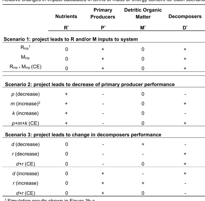
The first scenario simulated direct inputs of nutrients and detrital organic matter. 400
Results show that in all cases, R* and M* did not vary (despite their initial increase). On
401
the contrary, the variables representing living compartments, P* and D*, increased. 402
Results also show that the relative variation to the baseline, d, is identical for P* and D*
403
(both positive deviations, Table 1). Concerning processes at equilibrium, the primary 404
production and the primary producer mortality both increased, as well as the processes 405
of decomposition and recycling, since none of these parameters were affected by the 406
project implementation. 407
The second scenario simulates an impact which consists of the decrease in primary 408
producer performance. This could be due to the physiological capacities of the 409
organisms being affected by the project or because the environmental conditions limit 410
their expression (e.g. a strong increase in water column turbidity). In this situation, the 411
parameters affected are k and m (which increased), and p (which decreased). It should 412
be recalled that p was kept greater than m (p - m > 0), as per our parameter hierarchy. A 413
decrease of p and an increase of k (global decrease of primary productivity) always has 414
a negative effect on P* (hence on primary production), a positive effect on R*, and a 415
negative effect on D*. In both cases, the relative variations to the baseline, d, are 416
identical for P* and D*. An increase of m has a similar effect on P* and R*, but has a
417
negative effect on D*. The cumulative effect (p + m + k) is almost equal in magnitude to 418
the effect of a decrease in m, which is much higher (by several orders of magnitude) 419
than the effects of p and k. Effects of p and k are quite negligible, each having a typical 420
order of magnitude of the parameters in q. 421
The third and final scenario simulated a change in the decomposer activity. This could 422
be triggered by a change in taxonomic composition, and also by the action of chemical 423
substances released during the project. Decreases and increases in d and r were 424
simulated, first separately and then together. Changes in d and r have no effect on R*. A 425
decrease of d as a negative effect on P* (hence decreasing primary production) and D*, 426
and logically, an increase of d has a positive effect on P* (thus the increasing primary 427
production) as well as D*. In both cases, the relative variations to the baseline, d, are 428
identical for P* and D*. Effects of a decrease or an increase in r on P* and D* are
429
opposed. P* increases and D* decreases when r increases, and P* decreases and D* 430
increases when r decreases. Cumulative effects reinforce slightly the effect of a change 431
in r which is largely predominant in the dynamics of P and D. The changes of d and r 432
affect the primary production via a change in the availability of R. When the recycling 433
is enhanced (mainly by the increase of r but also by an increase of d), R production 434
increases but an excess of R is used to increase the state of the primary producer P. It is 435
because the production rate p is high compared to r, that R* is not affected by changes 436
in r or d. Changes in r and d have opposite effects on M*. A decrease (respectively,
437
increase) of d has a positive (respectively, negative) effect on M*, and a single decrease 438
(respectively, increase) of r has a negative (respectively, positive) effect on M*. When 439
changes are cumulated (in equal proportions), the effect of changes in r and d on M* is 440
null, showing that they have the same amplitude on M*.
441
Behaviour of system when drivers of change were included. In the impact
442
assessment per se, the effects of changes in ecosystems components (states and 443
functions) were considered as a deviation of stable equilibrium values regardless of the 444
time scales of the transitory phase. The consequences of introducing socio-economic 445
drivers were considered by numerical simulations. To take into account the potential 446
influence of socio-economic drivers, simulations were performed introducing explicitly 447
a changing rate that depends on the relative project activity within Equation 6, affecting 448
either states or parameters. Figure 3 shows results of simulations for just two different 449
examples of impact taken from Table 1. The first scenario illustrated (Figure 3b, c) is 450
for a project development that induces a change in state (a nutrient input triggering an 451
initial increase of R, scenario 1), and the second illustration (Figure 3d, e) suggests what 452
can occur when a project induces a change in parameters (in this case an increase in the 453
mortality rate of primary producers and hence a decrease of their survival, scenario 2). 454
The reactivity rate r was set to 0.02 (time-1) and the awareness rate s was set to 10-4
455
(time-1). For both scenarios, the project activity starts at t = 200 (time), the dynamics 456
being considered at steady state before. Figure 3a shows the activity of the project 457
reaches instantaneously 1 at ‘time’ 200 when the project is implemented and then 458
decreases smoothly as global awareness of negative impacts among stakeholders’ 459
increases [Eq. 8]. The project activity thus decreases to 0 by ‘time’ 800. This is a 460
consequence of the relative socio-economic cost of the project reaching 1, which in our 461
model, defines the limit of the exploitability of the project (i.e. when all possible time 462
and resources are being invested in side issues). 463
In the first scenario, when R increased sharply, both P and D increased as well, but 464
more slowly (Figure 3b). When the project activity stopped (outside the grey area, after 465
‘time’ 800), all states have reached an equilibrium, which is, for M, the equilibrium 466
prior to the implementation of the project, but for P and D, a different higher 467
equilibrium. In that sense, the outcome is similar to the outcome of the previous 468
scenario 1. Figure 3c shows that the d for P and D varies differently showing the 469
modulation by the project activity tends to alter the final amplitude of the impacts on 470
each of the receptors. 471
In the second scenario, the configurations for the relative socio-economic cost and 472
activity of the project are identical, but the outcomes were very different from those in 473
scenario 2. In this case, when project activity stopped, causes for changes in the 474
mortality rates disappeared and equilibrium states came back to the values prior to the 475
project implementation (Figures 3 d, e). Therefore, around ‘time’ 400, the impact of the 476
project on all receptors reaches a maximum, but all impacts relative to the baseline, d, 477
decreased and returned to zero afterward (Figure 3e). 478
479
DISCUSSION 480
The practice of EIA arose from a societal imperative to have documented expertise 481
about potential impacts on the environment from development projects. This was the 482
result of a legal framework created to defend environmental quality of communities and 483
regions in the US (Cashmore, 2004; Morgan, 2012), and coinciding with a rise in 484
visibility of ecological sciences (Supplementary Information, Figure A). Subsequently, 485
similar requirements for environmental impact assessment were adopted by a majority 486
of countries (Morgan, 2012). This has engendered repeated calls to develop a theory of 487
impact assessment (Lawrence, 1997) as the practice dispersed. The need for an EIA 488
process created a profession with a vital role in the safeguard of environmental quality, 489
but that relies heavily on disputable methods and has an uneven record (e.g. Wood, 490
2008; Wärnbäck and Hilding-Rydevik, 2009; Barker and Jones, 2013). Public pressure 491
from stakeholders may provide some measure of accountability, however, post hoc 492
analyses are rare (Lawrence, 1997) and systems can differ significantly between 493
countries (Lyhne et al., 2015). Critical review may only happen in the aftermath of a 494
dramatic accident, such as the Macondo well blow-out in 2010 (US Chemical Safety 495
and Hazard Investigation Board, 2016) or after management failures (Rotherham et al., 496
2011). 497
The value of quantification. Our study reflects on the two main scientific components
498
of EIAs: expertise and prediction. The first is the role of the expertise. We have stressed 499
the needs for the experts to identify receptors and to provide proper estimates of 500
baselines. The second one is the ability of ecological theory to prediction ecosystem 501
dynamics. We have emphasized the critical importance of the formulation of the 502
ecosystem model to calculate correctly baselines and predict impacts. The intention of 503
Leopold et al. (1971) was however far from this approach. Their approach consisted in 504
providing a sort of template for EIA and EIS documents and to ensure a common logic 505
for how the “magnitude and importance” of the impacts identified would be presented 506
to federal evaluators. They did not provide any details about how exactly impacts would 507
be assessed beyond a comparison between conditions before and after the project. We 508
therefore replaced this generic matrix approach by a quantification of system dynamics, 509
which allows scenarios to be designed and tested. 510
Receptor selection. Scenarios are selection of the possible combinations that could be
511
examined, and which are usually specific to the type of project that would be 512
implemented. The ecosystem model is then used as a tool to helps experts identifying 513
specific receptors. Receptors can only be identified if their ! is different from zero 514
(either strictly positive or strictly negative). It can be identified easily in Table 1, but 515
this is not the only condition: to be a receptor the ! must indeed be greater (in absolute 516
value) than the !* corresponding to the limit of detection of the impact [Eq 5]; this is a
517
statistical concept required to estimate the dispersion of the values of the receptor 518
variables around their average. These two conditions then define what receptors are. 519
Receptors are indeed subject to change and must be sensitive enough to be detectable 520
with the statistical tests applied. Hence, an EIA, in contrast with a risk assessment, 521
implies automatically a change in the receptors and aims to quantify them with a 522
defined level of certainty and accuracy. A consequence of this is that if two receptor 523
variables were identified as having the same dispersion, the impact will be better 524
assessed if the averages have higher values. For example, in a marine system, the 525
biomass of decomposers D, can be much greater than the biomass of the primary 526
producers, P (Simon et al., 1992), which means that it could be better to assess impact 527
on D, than on P. This can be completely different for terrestrial ecosystems (Cebrian 528
and Lartigue, 2004). 529
Baselines and reference conditions. In our model, the description of changes is based
530
on the calculation of equilibrium (the baseline) and their stability, and then follows the 531
displacement of the equilibrium values under changes in state variables, forcing 532
variables, or parameters (Figure 3b-e). This description is a basis for clarifying our 533
understanding of the problem. A dynamic model constrains our investigation to 534
plausible causal relationships between the variables (receptors) and permits us to 535
explore their contribution to the entire system. The dynamic behaviour provides a point 536
of reference for comparisons between scenarios (as shown in Table 1 and Figure 3), or 537
as they correspond to a specific project development. Formulating a minimum 538
ecosystem as an example, has shown that complex behaviours can emerge with only 539
four state variables. These results illustrate for the first time the dynamics of impact 540
responses by receptors, revealing how complicated the evaluation of recommendations 541
to mitigate impact may be. Furthermore, this underscores the importance of monitoring 542
to ensure accountability over the project life cycle, including cumulative effects. 543
Minimum ecosystems and complexity. Models are simulation tools which aid
544
exploration of possible outcomes and the evaluation of the simulated baseline, as well 545
as the relevance to simulated scenarios (Tett et al., 2011). Our minimum ecosystem 546
model is essentially a representation of a perfect and autonomous bioreactor, which 547
does not exist, nor can one be created as presented. Nutrients and detrital organic matter 548
are 100% recyclable by one functional group of decomposers. Populations are stable 549
indefinitely if conditions on the parameters (essentially p > m) are respected. These 550
conditions are not realistic, but serve the development and presentation of our approach. 551
The proposed procedures can be applied to more complex systems, encompassing large 552
quantity of variables (or compartments) as well as non-linear processes and hybrid 553
dynamics, like what would be expected in more realistic representations of ecosystems. 554
However, the condition that a certain form of stability can exist in the system must be 555
respected. It should be noted that the question of stability in ecology is part of an on-556
going scientific discussion recently summarized by Jacquet et al. (2016). This is critical 557
to environmental impact theory because it is the presumption of stability which ensures 558
the baseline is maintained (does not drift) during the project life cycle (Thorne and 559
Thomas, 2008; Pearson et al., 2012). In other words, an EIA is supposed to certify that 560
what is measured as change only corresponds to an impact from the project, not external 561
variations. Hence, monitoring takes on a new importance. For example, monitoring a 562
non-impacted site as a reference to detect possible ecosystem drift, may be one way to 563
assure that this condition of baseline stability is valid. This solution is conditioned itself 564
by the necessity to have a reference site which can be characterized by exactly the same 565
ecosystem. 566
The second basic assumption of our minimum ecosystem implies that the distribution of 567
elements is homogeneous inside the project area. This is not always (and even rarely) 568
the case and in aquatic systems, hydrodynamics leads to partial mixing that cannot be 569
assimilated to complete homogeneity. Therefore, accounting for the spatial distribution 570
structure of the elements would require the model structure be modified. For example, 571
we can use partial differential equations or any other formulation that can treat spatial 572
covariance. When spatial covariance is proven to exist for relevant receptors, the 573
corresponding statistics for the test of impact must account for the spatial covariance 574
using geostatistical methods (e.g. Agbayani et al., 2015; Wanderer and Herle, 2015). 575
Socio-ecological systems. The idea that all components (i.e. Environmental, Social,
576
Health … impacts) can be inserted into a single system framework remains quite 577
challenging. While a considerable number of propositions for conceptual frameworks 578
and planning charts exist (Haberl et al., 2009; Binder et al., 2013; Bowd et al., 2015; 579
Ford et al., 2015) offering some insights into the complex social interactions and policy 580
constraints involved, there is little in the way of theoretical development for impact 581
theory. We only studied here the project activity controlled by its socio-economic cost 582
(side costs being related to remediation and mitigation measures) as a driver of 583
ecosystem changes. We have not, for example, considered that changes in some 584
receptors can trigger an increase in cost and a decrease in activity. In other words, we 585
have not considered feedbacks between the receptors and cost, because it did not appear 586
clearly how awareness of stakeholders and reactivity of managers could be directly 587
linked to changes in receptors (Binder et al., 2013; Bowd et al., 2015) for which 588
“acceptable” remediation or mitigation measures should have already been considered 589
during the process (Figure 2B; Drayson and Thompson, 2013). Indeed, stakeholders’ 590
awareness depends on many factors, like information or education (Zobrist et al., 2009), 591
and reactivity of managers can be constraints by many other economic and political 592
factors (Ford et al., 2015). However, the minimal model that we proposed for 593
expressing the dynamics of the drivers of change [Equation 6] can (and should) become 594
more rich to take into account more complete descriptions of the mechanisms that 595
modulate awareness, activity and reactivity rates within sociological networks. We 596
suggest that our approach could be particularly useful in the scoping step as a means to 597
explore possible scenarios outcomes. 598
599
CONCLUSIONS 600
This study has linked statistical tests and mathematical modelling to assess an impact 601
and consider some of the socio-economic drivers that mitigate it. This constitutes a first 602
step toward an ecosystem-based approach for EIA, which needs to be proven and 603
improved. If technically, there are possibilities for EIA to rest on objective quantitative 604
approaches, these can only be valid if the predictive capacity of the model is assured. 605
This was, and still is, a major limitation. Furthermore, all forms of environmental 606
impact assessment are complicated by the absence of fundamental laws in ecology 607
(Lange, 2002) which has limited the understanding of complex objects in ecosystems. 608
Most of the time, ecosystem models simulate dynamics with properties that are not 609
found in realistic systems (May, 1977). We believe that to progress toward quantitative 610
EIA it is necessary to build much closer, interdisciplinary collaborations between 611
applied and fundamental research on ecosystems, to overcome the historical 612
divergences. This exchange could be encouraged through concrete measures such as 613
including funding for fundamental development within EIA as well as requiring that 614
data collected for IA be made available in open source repositories, accessible for 615 fundamental research. 616 617 SUPPLMENTARY MATERIAL 618
This material is not included in this version.
619
620
ACKNOWLEDGEMENTS 621
This work was presented in part at the ICES meeting “MSEAS2016” in Brest, France 622
and is part of the dissertation of J Coston-Guarini, inspired by the original insights of 623
Jody Edmunds. 624
REFERENCES 626
Adler, P. B., Fajardo, A., Kleinhesselink, A. R., and Kraft, N. J. B. 2013. Trait-based 627
tests of coexistence mechanisms. Ecology Letters, 16: 1294-1306. 628
Agbayani, S., Picco, C. M., and Alidina, H. M. 2015. Cumulative impact of bottom 629
fisheries on benthic habitats: A quantitative spatial assessment in British Columbia, 630
Canada. Ocean & Coastal Management, 116: 423-444. 631
Barker, A., and Jones, C. 2013. A critique of the performance of EIA within the 632
offshore oil and gas sector. Environmental Impact Assessment Review, 43: 31-39. 633
Beaumont, N. J., Austen, M. C., Mangi, S. C., and Townsend, M. 2008. Economic 634
valuation for the conservation of marine biodiversity [Viewpoint]. Marine Pollution 635
Bulletin, 56: 386-396. 636
Berkes, F., and Folke, C. 1998. Ch. 1 Linking social and ecological systems for 637
resilience and sustainability. In Linking sociological and ecological systems: 638
management practices and social mechanisms for building resilience, pp. 1-26. Ed. by 639
F. Berkes, C. Folke, and J. Colding. Cambridge University Press, New York. 476 pp. 640
Binder, C. R., Hinkel, J., Bots, P. W. G., and Pahl-Wostl, C. 2013. Comparison of 641
frameworks for analyzing social-ecological systems. Ecology and Society, 18(4): 26. 642
Bowd, R., Quinn, N. W., and Kotze, D. C. 2015. Toward an analytical framework for 643
understanding complex social-ecological systems when conducting environmental 644
impact assessments in South Africa. Ecology and Society, 20(1): 41. 645
646
Buttel, F. H., and Flinn, W. L. 1976. Social class and mass environmental beliefs: a 647
reconsideration [Rural Sociological Society Annual Meeting, New York]. Michigan 648
Agricultural Experiment Station Journal, 7749: 1-12. 649
Cashmore, M. 2004. The role of science in environmental impact assessment: process 650
and procedure versus purpose in the development of theory. Environmental Impact 651
Assessment Review, 24: 403-426. 652
Cashmore, M., Richardson, T., Hilding-Rydevik, T., and Emmelin, L. 2010. Evaluating 653
the effectiveness of impact assessment instruments: Theorising the nature and 654
implications of their political constitution. Environmental Impact Assessment Review, 655
30: 371-379. 656
Cebrian, J., and Lartigue, J. 2004. Patterns of herbivory and decompostion in aquatic 657
and terrestrial ecosystems. Ecological Monographs, 74(2): 237-259. 658
de Lacaze-Duthiers, F. J. H. 1881. Les progrès de la station zoologique de Roscoff et la 659
creation du Laboratoire Arago à Banyuls-sur-Mer. Archives de Zoologie Expérimentale 660
et Générale, Série 1, Tome IX: 543-598. 661
Drayson, K., and Thompson, S. 2013. Ecological mitigation measures in English 662
Environmental Impact Assessment. Journal of Environmental Management, 119: 103-663
110. 664
Edmunds, J., Hinz, S., Wilson, J., Guarini, J., Van Colen, C., and Guarini, J.-M. 2016. 665
A novel interdisciplinary approach to building system based environmental impact 666
assessments for marine and aquatic environments. In Abstract Book. Second Mares 667
Conference: Marine Ecosystems Health and Conservation, February 1st - 5th 2016, 668
Olhão, Portugal, pp. 149. Ed. by K. Brownlie. Ghent University, Marine Biology 669
Research Group/Centre of Marine Sciences (CCMAR), University of Algarve, Ghent. 670
163 pp. 671
Ford, A. E. S., Graham, H., and White, P. C. L. 2015. Integrating human and ecosystem 672
health through ecosystem services frameworks. EcoHealth, 12: 660-671. 673
Gause, G. F. (1934). The Struggle for Existence. Williams & Wilkins Company, 674
Baltimore. 163 pp. 675
Gillette, R. 1971. Trans-Alaska Pipeline: Impact study receives bad reviews. Science, 676
171: 1130-1132. 677
Gómez-Baggethun, E., de Groot, R., Lomas, P. L., and Montes, C. 2010. The history of 678
ecosystem services in economic theory and practice: From early notions to markets and 679
payment schemes. Ecological Economics, 69(6): 1209-1218. 680
Goodstein, D. 2011. How Science Works. In Reference Manual on Scientific Evidence: 681
Third Edition, pp. 37-54. Ed. by Committee on the Development of the Third Edition of 682
the Reference Manual on Scientific Evidence, the Federal Judicial Center, and the 683
National Research Council. National Academies Press, Washington DC. 1038 pp. 684
Gray, P. C. R., and Wiedemann, P. M. 1999. Risk management and sustainable 685
development: mutual lessons from approaches to the use of indicators. Journal of Risk 686
Research, 2(3): 201-218. 687
Haberl, H., Gaube, V., Díaz-Delgado, R., Krauze, K., Neuner, A., Peterseil, J., Plutzar, 688
C., Singh, S. J., and Vadineanu, A. 2009. Towards an integrated model of 689
socioeconomic biodiversity drivers, pressures and impacts. A feasibility study based on 690
three European long-term socio-ecological research platforms. Ecological Economics, 691
68: 1797-1812. 692
Holling, C. S. 1959. Some characteristics of simple types of predation and parasitism. 693
The Canadian Entomologist, 91(7): 385-398. 694
Jacobsen, N. S., Essington, T. E., and Andersen, K. H. 2016. Comparing model 695
predictions for ecosystem based management. Canadian Journal of Fisheries and 696
Aquatic Sciences, 73(4): 666-676. 697
Jacquet, C., Moritz, C., Morissette, L., Legagneux, P., Massol, F., Archambault, P., and 698
Gravel, D. 2016. No complexity–stability relationship in empirical ecosystems. Nature 699
Communications, 7: 12573. 700
Justus, J. 2008. Ecological and Lyapunov Stability. Philosophy of Science, 75: 421-436. 701
Lange, M. 2002. Who’s afraid of ceteris-paribus laws? Or: How I learned to stop 702
worrying and love them. Erkenntnis, 57: 407-423. 703
Lawrence, D. P. 1997. The need for EIA theory-building. Environmental Impact 704
Assessment Review, 17: 79-107. 705
Leopold, L. B., Clarke, F. E., Hanshaw, B. B., and Balsley, J. R. 1971. A procedure for 706
evaluating environmental impact. USGS Circular, N° 645: 13 pp. 707
Levins, R. 1974. The qualitative analysis of partially specified systems. Annals of the 708
New York Academy of Sciences, 231: 123-138. 709
Lyhne, I., van Laerhoven, F., Cashmore, M., and Runhaar, H. 2015. Theorising EIA 710
effectiveness: A contribution based on the Danish system. Environmental Impact 711
Assessment Review. 712
Marsh, G. P. (1865). Physical Geography as modified by human action. New York: 713
Charles Scribner. 560 pp. 714
May, R. M. 1977. Thresholds and breakpoints in ecosystems with a multiplicity of 715
stable states. Nature, 269: 471-477. 716
McIntosh, R. P. (1985). The Background of Ecology: Concept and Theory. Cambridge 717
Univ Press. 383 pp. 718
Moreno-Mateos, D., Power, M. E., Comín, F. A., and Yockteng, R. 2012. Structural and 719
functional loss in restored wetland ecosystems. PLOS Biology, 10(1): e1001247. 720
Morgan, R. K. 2012. Environmental impact assessment: the state of the art. Impact 721
Assessment and Project Appraisal, 30(1): 5-14. 722
Nouri, J., Jassbi, J., Jafarzadeh, N., Abbaspour, M., and Varshosaz, K. 2009. 723
Comparative study of environmental impact assessment methods along with a new 724
dynamic system-based method. African Journal of Biotechnology, 8(14): 3267-3275. 725
Odum, E. P. 1969. The strategy of ecosystem development. Science, 164(3877): 262-726
270. 727
Odum, E. P. 1975. Ecology: The link between the natural the social sciences. 2nd edn. 728
Holt, Rinehard and Winston, New York. 234 pp. 729
Odum, E. P. 1977. The emergence of Ecology as a new integrative discipline. Science, 730
195(4284): 1289-1293. 731
Odum, H. T. 1957. Trophic structure and productivity of Silver Springs, Florida. 732
Ecological Monographs, 27(1): 55-112. 733
Payraudeau, S., and van der Werf, H. M. G. 2005. Environmental impact assessment for 734
a farming region: a review of methods. Agriculture, Ecosystems & Environment, 735
107(1): 1-19. 736
Pearson, W. H., Deriso, R. B., Elston, R. A., Hook, S. E., Parker, K. R., and Anderson, 737
J. W. 2012. Hypotheses concerning the decline and poor recovery of Pacific herring in 738
Prince William Sound, Alaska. Reviews in Fish Biology and Fisheries, 22(1): 95-135. 739
Peterson, M. J., Hall, D. M., Feldpausch-Parker, A. M., and Peterson, T. R. 2009. 740
Essay: Obscuring ecosystem function with application of the ecosystem services 741
concept. Conservation Biology, 24(1): 113-119. 742
Pope, J., Bond, A., Morrison-Saunders, A., and Retief, F. 2013. Advancing the theory 743
and practice of impact assessment: Setting the research agenda. Environmental Impact 744
Assessment Review, 41: 1-9. 745
Rissman, A. R., and Gillon, S. 2016. Where are Ecology and Biodiversity in Social– 746
Ecological Systems Research? A Review of Research Methods and Applied 747
Recommendations. Conservation Letters, : 1-8. 748
Rotherham, D., Macbeth, W. G., Kennelly, S. J., and Gray, C. A. 2011. Reducing 749
uncertainty in the assessment and management of fish resources following an 750
environmental impact. ICES Journal of Marine Science, 68(8): 1726-1733. 751
Ryabov, A. B., and Blasius, B. 2011. A graphical theory of competition on spatial 752
resource gradients. Ecology Letters, 14: 220-228. 753
SciLab Enterprises. 2012. Scilab: Free and Open Source software for numerical 754
computation (Version 5.2.2) [Software]. Available from: http://www.scilab.org 755
Simon, M., Cho, B. C., and Azam, F. 1992. Significance of bacterial biomass in lakes 756
and the ocean: comparison to phytoplankton biomass and biogeochemical implications. 757
Marine Ecology Progress Series, 86: 103-110. 758
Smith, A. D. M., Fulton, E. J., Hobday, A. J., Smith, D. C., and Shoulder, P. 2007. 759
Scientific tools to support the practical implementation of ecosystem-based fisheries 760
management. ICES Journal of Marine Science, 64: 633-639. 761
Tansley, A. G. 1935. The use and abuse of vegetational concepts and terms. Ecology, 762
16(3): 284-307. 763
Tett, P., Ribeira d’Acalà, M., and Estrada, M. 2011. Chapter 4. Modelling coastal 764
systems. In Sustaining Coastal Zone Systems, 1st edn, pp. 79-102. Ed. by P. Tett, A. 765
Sandberg, and A. Mette. Dunedin Academic Press, Edinburgh. 166 pp. 766
Thorne, R. E., and Thomas, G. L. 2008. Herring and the “Exxon Valdez” oil spill: an 767
investigation into historical data conflicts. ICES Journal of Marine Science, 65(1): 44-768
50. 769
Toro, J., Duarte, O., Requena, I., and Zamorano, M. 2012. Determining Vulnerability 770
Importance in Environmental Impact Assessment The case of Colombia. Environmental 771
Impact Assessment Review, 32: 107-117. 772
Toro, J., Requena, I., Duarte, O., and Zamorano, M. 2013. A qualitative method 773
proposal to improve environmental impact assessment. Environmental Impact 774
Assessment Review, 43: 9-20. 775
Tzanopoulos, J., Mouttet, R., Letourneau, A., Vogiatzakis, I. N., Potts, S. G., Henle, K., 776
Mathevet, R., and Marty, P. 2013. Scale sensitivity of drivers of environmental change 777
across Europe. Global Environmental Change, 23: 167-178. 778
UNEP. (2005). Ecosystems and Human Well-Being: Current State & Trends, Volume 779
1. United Nations Environment Program. 900 pp. 780
US Chemical Safety and Hazard Investigation Board. (2016). Investigation Report. 781
Executive Summary. Drilling rig explosion and fire at the Macondo Well. 24 pp. 782
Wanderer, T., and Herle, S. 2015. Creating a spatial multi-criteria decision support 783
system for energy related integrated environmental impact assessment. Environmental 784
Impact Assessment Review, 52: 2-8. 785
Wärnbäck, A., and Hilding-Rydevik, T. 2009. Cumulative effects in Swedish EIA 786
practice — difficulties and obstacles. Environmental Impact Assessment Review, 29: 787
107-115. 788
Wood, G. 2008. Thresholds and criteria for evaluating and communicating impact 789
significance in environmental statements: ‘See no evil, hear no evil, speak no evil’? 790
Environmental Impact Assessment Review, 28: 22-38. 791
Židonienė, S., and Kruopienė, J. 2015. Life Cycle Assessment in environmental impact 792
assessments of industrial projects: towards the improvement. Journal of Cleaner 793
Production, 106: 533-540. 794
Zobrist, J., Sima, M., Dogaru, D., Senila, M., Yang, H., Popescu, C., Roman, D., Bela, 795
A., Frei, L., Dold, B., and Balteanu, D. 2009. Environmental and socioeconomic 796
assessment of impacts by mining activities—a case study in the Certej River catchment, 797
Western Carpathians, Romania. Environmental Science and Pollution Research, 798 16(Supplement 1): 14-26. 799 800 801
TABLE 802
Table 1. Summary of model outcomes for three scenarios. Relative changes in
803
impact are calculated in terms of mass or energy content and compared for the scenarios 804
described in the results. 805
806
FIGURES 807
Figure 1. Environmental impact assessment, then and now.
808
(a) The original flow chart as it appeared in Leopold et al. 1971. This chart responds to 809
a specific request by the US Department of the Interior to propose a system that would 810
structure information in EI documents. The original figure is captioned: “Evaluating the 811
environmental impact of an action program or proposal is a late step in a series of 812
events which can be outlined in the following manner.” 813
(b) Example of a flow chart used by consultants today in offshore projects. Important 814
changes include: the addition monitoring and the possibility of using modeling. Steps 815
external to the core EIA steps are in grey. Redrawn after Edmunds et al. 2016. 816
Figure 2. The minimum ecosystem model.
817
(a) The simplest representation of a model in ecology requires two state variables at 818
least one parameter and a ‘forcing’ variable to describe the external forcing by dynamic 819
environmental conditions such as light, temperature, tides. State variables 820
(compartments) are written as a function of the parameters, forcing variables, or other 821
state variables, for a given time interval. Because these vary dynamically they are 822
written as differential equations. Forcing variables are fixed externally, and are not 823