An agent-based approach to modeling electricity spot markets

(1)

An Agent-based Approach to Modeling Electricity Spot

Markets

by

Poonsaeng Visudhiphan

B.Eng., Electrical Engineering,

Chulalongkorn University, Bangkok, Thailand (1995) M.S., Electrical Engineering and Computer Science,

Massachusetts Institute of Technology (1998)

Submitted to the Department of Electrical Engineering and Computer Science in partial fulfillment of the requirements for the degree of

Doctor of Philosophy at the

MASSACHUSETTS INSTITUTE OF TECHNOLOGY MASSAcHUSETS ZSTITUTE

May 2003 OF TECHNOLOGY

J UL 0 7 200

@

2003 Massachusetts Institute of Technology 003

LIBRARIES

A u th or ... ...

Department of Electrical Engineering and Computer Science

April 23, 2003 Certified by... Department of Electrical Senior Engineering and ... Marija D. Ilid Research Scientist Computer Science Thesis Supervisor Accepted by ... ... Departme .. ... ... , Z a .. . Arthur C. Smith Chairman, Committee on Graduate Students nt of Electrical Engineering and Computer Science

(2)

(3)

An Agent-based Approach to Modeling Electricity Spot Markets

by

Poonsaeng Visudhiphan

B.Eng., Electrical Engineering,

Chulalongkorn University, Bangkok, Thailand (1995)

M.S., Electrical Engineering and Computer Science,

Massachusetts Institute of Technology (1998)

Submitted to the Department of Electrical Engineering and Computer Science on April 23, 2003, in partial fulfillment of the

requirements for the degree of Doctor of Philosophy

Abstract

Current approaches used for modeling electricity spot markets are static oligopoly models that pro-vide top-down analyses without considering dynamic interactions among market participants. This thesis presents an alternative model, an agent-based model, and uses it to analyze the markets under various conditions. These markets, in which the participants engage in sealed-bid auctions to sell and/or buy electricity regularly, are viewed as multiagent systems, or as repeated games, played by participants with incomplete information. To represent these market characteristics, the agent-based model is selected, consisting of several power-producing agents with non-uniform portfolios of generat-ing units. These agents employ learngenerat-ing algorithms, includgenerat-ing Auer et al.'s, softmax action selection, or Visudhiphan and Ili6's model-based algorithms, in determining bid-supply functions from available information.

The simulated outcomes from the agent-based model depend on the choice of non-uniform port-folios and on the learning algorithms that the agents employ. Model verifications against the actual markets are suggested; however, due to a lack of certain confidential information, numerical examples cannot be presented. Nevertheless, the model is used to analyze the effects of market structures and the effect of load-serving entities on the power-producer bidding behavior and market outcomes.

This model could provide one of the main tools for regulators, system planners, and market participants to use scenario simulations to investigate market conditions that could lead to high electricity prices. The model could also be used to analyze market factors (such as new market rules) and their effects on market price dynamics and market participants' behaviors, as well as to identify the "best" response action of one participant against the opponents' actions.

Thesis Advisor: Prof. Marija D. Ili.

Thesis Committee Members: Prof. Leslie P. Kaelbling, Prof. John N. Tsitsiklis, and Dr. Robert F. Brammer (Northrop Grumman TASC).

(4)

(5)

Acknowledgments

I would like to thank several people who have been helping, supporting, and encouraging me through-out my graduate study. Prof. Marija D. I1i, my thesis advisor and my mentor, who has so much passion in her research, has been my inspiration in accomplishing this work. I have gained invaluable experience from working with Prof. Ilid in addressing challenging and practical problems in evolving electricity markets. Prof. Leslie Kaelbling, Prof. John Tsitsiklis, and Dr. Robert Brammer (Northrop Grumman TASC), my thesis committee members deserve my special thanks. They provided wonder-ful comments on my work, especially those related to game theory, learning algorithms, and empirical studies. Additional thanks go to Prof. Kaelbling kindly served as my EECS Area Exam chairman.

I would like to gratefully thank several institutions and organizations for their generous financial support over the course of my graduate study. Without their support, my research would not have been possible. They include the Government of Japan, the members of the MIT Consortium on "New Concepts and Software for Competitive Power Systems, MIT Department of Electrical Engineering and Computer Science, the MIT EECS Alumni Fund, and the ABB Power T&D Company.

I would like to thank several professors and students of Prof Iliks, especially Jill Watz, Katherine Millis, Jeff Chapman, Chen-ning Yu, Petter Skantze, Yong Tae Yoon, Santosh Raikar, Jason Black, and Mrdjan Mladjan. Without them my graduate study at MIT would not be as challenging and intellectually stimulating. I am very grateful to the staffs at the EECS graduate office, especially Marilyn Pierce and Peggy Carney, at the Energy Lab, and at LIDS, especially Fifa Monserrate, for providing help whenever I asked. I also would like to thank the staff members at the MIT writing center, especially Thalia Rubio, for their help in editing and revising my thesis.

I am also grateful to David Chargin, his family, and several wonderful friends, especially Ariya Akthakul, Tengo (Poompat) Saengudomlert, Yot Boontongkong, and Lorraine Gray; they made my graduate-student life no less than excellent. My thanks go to other Thai friends and colleagues at the Energy lab and LIDS for their friendship and support. I feel very grateful for the warm welcome and hospitality of Sarah Wise and Donna and Allen Buchholz that I have received since I came to the United States several years ago. Lastly, I would like to thank my family, who have been truly encouraging and supporting me to reach any goal I attempt.

(6)

(7)

4.1 M arket M odel . . . .. 4.1.1 Characteristics of Agents . . . .. 4.1.2 Characteristics of Demand . . . . 4.1.3 M arket Rules . . . . 4.2 Agents with Algorithms Al, A2, and A3 . . . . 4.2.1 Algorithms Al and A2 . . . . 4.2.2 Algorithm A3 . . . . 4.2.3 Analyses . . . . 4.3 Agents with Algorithm SAB . . . . 4.3.1 Effects of T on Price Dynamics . . . . 4.3.2 Effects of a on Price Dynamics . . . . 4.3.3 Analyses . . . . 4.4 Agents with the Model-based Algorithm . . . . 4.4.1 Choosing Tar by Methods M1 and M2 . . . . 4.4.2 Effects of A on Price Dynamics . . . . 4.4.3 Effects of WHk on Price Dynamics . . . . 4.4.4 Analyses . . . . 4.4.5 Simulations with a Game Matrix . . . . 4.5 Learning Algorithms and Bidding Behavior . . . . . 4.5.1 Analyzing Algorithm A3 . . . . 4.5.2 Algorithm A3 and the Model-based Algorithm 4.6 Exploring the Model . . . .

4.6.1 Price-war . . . . 4.6.2 Dominant Agent . . . . 4.6.3 Unit-by-unit vs. Portfolio Decision Scheme . 4.7 Verification of Agent-based Market Model . . . . 4.7.1 Average Square Error . . . . 4.7.2 Probability of Correctness . . . . 4.7.3 Insufficient Information . . . . 4.8 Conclusion . . . . 75 76 79 82 93 93 94 94 95 96 96 97 97 98 99 99 99 100 100 101 101 101 104 106 106 108 109 109 111 112 116 116 117 118 119

(9)

5 Analyzing the New England Electricity Market

5.1 Analyzing Bidder Behavior

5.2 Identifying Marginal Units ...

5.2.1 Results . . . . 5.3 Lead Participant Bidding Behavior . .

5.3.1 Observing Bidding Behavior.

5.3.2 Observation and Analyses . . 5.4 Load Indices and Bidding Behavior

5.4.1 A Possible Bidding Strategy

5.4.2 Observation and Analysis .

5.5 Bidding Behavior of Generating Units

5.5.1 Bidding Behavior . . . ..

5.5.2 Observation and Analysis . . .

5.6 Conclusion . . . .

6 Applications of the Agent-based Market Model

6.1 Uniform and Discriminatory-pricing Markets . . . .

6.1.1 M odels . . . . 6.1.2 Sim ulations . . . .

6.1.3 A nalyses . . . . 6.1.4 Implications of the Simulations . . . .

6.2 The Role of Load-serving Entity . . . . 6.2.1 M odels . . . . 6.2.2 Preliminary Analysis . . . .

6.2.3 Sim ulations . . . . 6.2.4 A nalyses . . . .

6.2.5 Comments and Conclusions . . . .

7 Possible Future Research and Conclusions

7.1 Contributions of the Agent-based Model . . . .

7.2 Future Work . . . . 7.2.1 Model Improvement . . . .

7.2.2 A Simplified Method for Reproducing Market Prices . 7.2.3 Effects of Demand Uncertainties . . . .

7.3 Conclusions . . . . . . . . 2 5 7 9

. . . .

145 146 149 150 152 153 155 157 158 161 161 162 164 166 191 192 192 194 194 197 198 199 208 211 213 216 251 252 252 252 254 255

(10)

A Available Information and Spot Prices A.1 General Background ...

A.2 PMF of Prices Given Demand: Case I . . . . A.2.1 Known Number of Unavailable Units . . . . A.2.2 Imperfect Competition . . . .

A.2.3 Simulations . . . .

A.2.4 Observations . . . . A.3 PMFs of Prices Given Demand: Case II . . . . A.3.1 PMFs of Prices Given Load . . . .

A.3.2 Simulations and Analyses . . . . A.3.3 Observation . . . . A.4 Imperfect Competition with Elastic Demand . . .

A.4.1 PMFs of Prices Given Elastic Demand . . .

A.4.2 Simulations and Analyses . . . .

A.5 Effects of Unit-commitment Constraints on Prices A.6 Possible Extension . . . .

261 . . . . 262 . . . 264 . . . 266 . . . . 270 . . . . 272 . . . 276 . . . 277 . . . . 277 . . . . 281 . . . . 283 . . . . 284 . . . . 288 . . . . 289 . . . . 290 . . . . 293

B Samples of MATLAB Codes 295

(11)

List of Figures

0-1 Load and bidding prices for quantity 2,000 MW of LP 506459 during January 18-31, 2000 ... ... 25 0-2 Load and bidding prices for quantity 1,000 MW of LP 218387 during January 18-31,

2000 ... ... 25 0-3 A scatter plot of sampled hourly loads and market prices during May 1, 1999 - April

30, 2001 ... ... 26 0-4 A histogram of hourly market prices during May 1, 1999 - April 30, 2001 . . . . 26

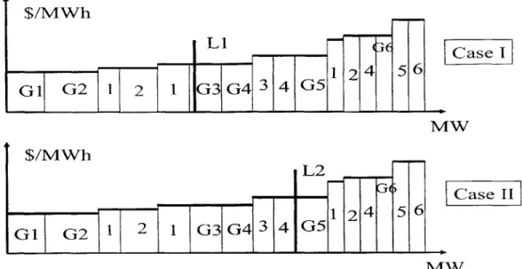
3-1 Examples of Different Power Producers Competing to Sell Electricity at Different De-m and Levels . . . . 89 3-2 An Example of Yearly Demand Characteristics in the New England Electricity Market

from M ay, 1999 to April, 2000 . . . . 89 3-3 Mapping Demand to Load Indices . . . . 90 3-4 Histogram of Hourly Market Prices in New England When Demand is within a 10,000

- 11,000 MW Range from May 1, 1999 to April 30, 2001 . . . . 90 3-5 Histogram of Hourly Market Prices in New England When Demand is within a 15,000

- 16,000 MW Range from May 1, 1999 to April 30, 2001 . . . . 91 3-6 Demand-supply Ratio and Associated Market-clearing Prices from May 1, 1999 to

Oc-tober 31, 1999 ... ... 91

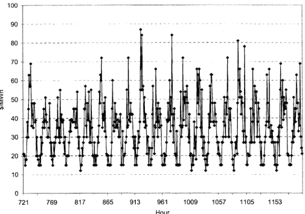
4-1 Aggregate Marginal-cost Function of the Hypothetical Market . . . 121 4-2 Hourly Inelastic and Deterministic Demands and Marginal-cost Prices . . . . 121 4-3 Price Dynamics from Hours 721 to 1,200 When the Agents Employ Algorithm Al with

y = 0 .1 . . . 122 4-4 Price Dynamics from Hours 721 to 1,200 When the Agents Employ Algorithm Al with

= 0.9 . . . 122 4-5 Price Dynamics from Hours 721 to 1,200 When the Agents Employ Algorithm A2 . . 123

(12)

4-6 Price Dynamics from Hours 721 to 1,200 When the Agents Employ Algorithm A3 with

3 = 0 .1 . . . . 4-7 Price Dynamics from Hours 721 to 1,200 When the Agents Employ Algorithm A3 with

3 = 0 .5 . . . . 4-8 Price Dynamics from Hours 721 to 1,200 When the Agents Employ Algorithm A3 with

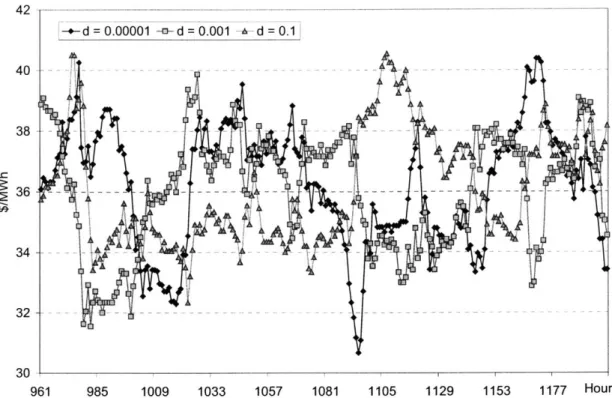
6 = 0 .9 . . . . 4-9 Moving-average Prices from Hours 721 to 1,200 When the Agents Employ Algorithm

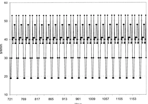
A3 with 6 = 0.1,0.001, and 0.00001 . . . . 4-10 Price Dynamics from Hours 721 to 1,200 When the Agents Employ Algorithm SAB

with a=0.9and-r= 1 . . 4-11 Price Dynamics from Hours with a = 0.9 and T = 10 . 4-12 Price Dynamics from Hours

with a = 0.9 and r = 100

4-13 Price Dynamics from Hours with a = 0.1 and T = 100

4-14 Price Dynamics from Hours with a = 0.5 and T = 100

4-15 Price Dynamics from Hours with a = 0.1 and r = 10 .

721 to 1,200 When the Agents Employ Algorithm SAB .7 . . . . .2 . . . .t . A. . . . .

721 to 1,200 When the Agents Employ Algorithm SAB .7 . . . .1.2 . . . .t . . . .

721 to 1,200 When the Agents Employ Algorithm SAB

4-16 Average Price Dynamics across 100 Simulations during Hours 961

-Agents Employ Algorithm A3 with 3 = 0.1 . . . . 4-17 Average Price Dynamics across 100 Simulations from Hours 961 to Agents Employ Algorithm SAB with a = 0.1 and r = 100 . . . . .

1,200 When the . . . . 1,200 When the

4-18 Price Dynamics from Hours 721 to 1,200 When the Agents Employ the Model-based Algorithm with Methods M1 and C2, and A = 2 . . . . 4-19 Price Dynamics from Hours 721 to 1,320 When the Agents Employ the Model-based

Algorithm with Methods M2 and C2, and A = 2 . . . . 4-20 Price Dynamics from Hours 721 to 1,200 When the Agents Employ the Model-based

Algorithm with A = 1 and Methods M1 and C2 . . . . 4-21 Price Dynamics from Hours 721 to 1,200 When the Agents Employ the Model-based

Algorithm A = 3 and Methods M1 and C2 . . . . 4-22 Daily Price Dynamics at Hour 8 When the Agents Employ the Model-based Algorithm

with Method M1 and A = 1, 2, and 3 . . . . 4-23 Daily Profits that Agent 1 Obtains at Hour 8 When the Agents Employ the Model-based

Algorithm with A = 1, 2, and 3 . . . . 123 124 124 125 125 126 126 127 127 128 128 129 129 130 130 131 131 132 . . . .

(13)

4-24 Daily Profits that Agent 5 Obtains at Hour 8 When the Agents Employ the Model-based Algorithm with A = 1, 2, and 3 . . . 132 4-25 Samples of Simulated Prices When the Agents Employ the Model-based Algorithm with

Method C1 or C2 to Determine WH . . . 133 4-26 Price Dynamics When the Agents Employ the Model-based Algorithm with Method

and M 2 a GM M atrix . . . 133 4-27 Price Dynamics When the Agents Employ the Model-based Algorithm with Method

M 1 and a GM M atrix . . . 134 4-28 Cumulative Profits that Agent 1 Obtains When It Submits a Particular Bid-supply

Function in Response to the Opponents Employing Algorithm A3 . . . 134 4-29 Cumulative Profits When Agent 1 Employs either Algorithm A3 or When It Submits

a Bid-supply Function with q = 6 MW and BM =$39/MWh . . . 135 4-30 Price Dynamics Obtained When Demand is equal to 66 MW, and either Agent 1 or 5

Employs a Learning Algorithm . . . 135 4-31 Price Dynamics from Hours 721 to 1,200 When the Agents Employ Algorithm A3 with

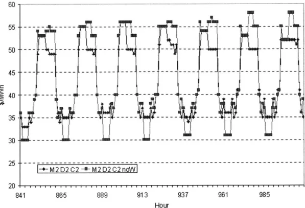
3 = 0.9 or Algorithm SAB with a = 0.9 and r 100 to Determine Only BM . . . . 136 4-32 Price Dynamics from Hours 841 to 1,008 When the Agents Employ the Model-based

Algorithm with Method Ml and A = 2 to Determine Only BM . . . 136 4-33 Price Dynamics from Hours 841 to 1,008 When the Agents Employ the Model-based

Algorithm with Method M2 and A = 2 to Determine Only BM . . . 137 4-34 Relationship between MP, (OP - AP), and BM of the Agents at Hour 4 from Days

1

to 6 When the Agents Employ the Model-based Algorithm with Method M2 . . . 137 4-35 Relationship between MP, (OP - AP), and BM of the Agents at Hour 4 from Days 1

-6 when the Agents Employ the Model-based Algorithm Without the CW Strategy . 138 4-36 Price Dynamics from Hours 721 to 1,200 When Only Agent 5 Employs Algorithm A3

with

6

= 0.9, While the Other Agents Submit their Marginal-cost Bids . . . 138 4-37 Price Dynamics from Hours 721 to 1,200 When Only Agent 5 Employs Algorithm SAB

with a = 0.9 and

r

= 100, While the Other Agents Submit Their Marginal-cost Bids 139 4-38 Price Dynamics from Hours 721 to 960 When Agent 5 Employs the Model-based

Algo-rithm with Methods M1 and C1 and A = 2, While the Agents Submit Their Marginal-cost B ids . . . 139 4-39 Price Dynamics from Hours 721 to 960 When Agent 1 Employs the Model-based

Algo-rithm with Methods M1 and C1 and A = 2, While the Agents Submit Their Marginal-cost B ids . . . 140 4-40 Price Dynamics from Hours 721 to 888 When the Agents Employ the Model-based

Algorithm with a Unit-by-unit Decision Scheme . . . 140

(14)

4-41 Price Dynamics from Hours 721 to 888 When the Agents Employ the Model-based Algorithm with Unit-by-unit or Portfolio-based Schemes, with Methods M1 and C1

and A= 2 ... ... 141

4-42 Price Dynamics from Hours 721 to 888 When the Agents Employ the Model-based Algorithm with Unit-by-unit or Portfolio-based Schemes, with Methods MI and A = 2 without the CW Strategy . . . 141

4-43 Price Dynamics from Hours 793 to 960 When the Agents Employ the Model-based Algorithm with Unit-by-unit or Portfolio-based Schemes, with Methods M2 and A = 2 without the CW Strategy . . . . 142

4-44 Prices and Bidding Prices of Agents 1 and 6 at Hour 7 Daily When the Agents Employ the Model-based Algorithm with a Unit-by-unit Decision Scheme, Methods M2 and U2, and A= 2 ... ... 142

4-45 (OP-AP) of Agents 1 and 6 at Hour 7 Daily When the Agents Employ the Model-based Algorithm with a Unit-by-unit Decision Scheme, Methods M2 and U2, and A = 2 . . 143

5-1 Examples of Hourly Bid-supply Functions of LP 506459 in January 2000 . . . 174

5-2 Examples of Hourly Aggregate Bid-supply Functions in January 2000 . . . 174

5-3 A Band of Marginal Units When Demand is Equal to 16,000 MW . . . 175

5-4 Daily Forecast Demand in New England during January 18-31, 2000 . . . 176

5-5 Daily Forecast Demand in New England during April 17-30, 2000 . . . 176

5-6 Daily Forecast Demand in New England during July 18-31, 2000 . . . 177

5-7 Daily Forecast Demand in New England during October 18-31, 2000 . . . . 177

5-8 Sampled Bidding Prices for some Bidding Quantities of LP 206845 during January 18-24, 2000 ... ... 178

5-9 Bidding Prices for some Bidding Quantities of LP 206845 during April 17-23, 2000 . . 178

5-10 Scheduled Quantities of LP 206845 during Four Two-week Periods of Study . . . 179

5-11 Self-scheduled Quantities of LP 206845 at Hour 14 during Four Two-week Periods of Study ... ... ... 179

5-12 Sampled Bidding Prices for Some Bidding Quantities of LP 218387 during January 18-24, 2000 ... ... 180

5-13 Sampled Bidding Prices for Some Bidding Quantities of LP 218387 during April 17-23, 2000 ... ... 180

(15)

5-16 Sampled Bidding Prices for Some Bidding Quantities of LP 506459 during April 17-23, 2000 .... ... ... 182 5-17 Sampled Bidding Prices for Some Bidding Quantities of LP 506459 during October

18-24, 2000 ... ... 182 5-18 Sampled Bidding Prices for Some Bidding Quantities of LP 506459 during July 18-24,

2000 . . . 183 5-19 Sampled Bidding Prices for Some Bidding Quantities of LP 506459 during July 25-31,

2000 ... ... 183 5-20 Scheduled Quantities of LP 506459 and Calculated Prices during January 18-31, 2000 184 5-21 Scheduled Quantities of LP 506459 and Calculated Prices during July 18-31, 2000 . . 184 5-22 Sampled Bidding Prices for Some Bidding Quantities of LP 529988 during January

18-24, 2000 ... ... 185 5-23 Sampled Bidding Prices for Some Bidding Quantities of LP 529988 during April 17-23

, 2000 ... ... 185 5-24 Sampled Bidding Prices for Some Bidding Quantities of Asset ID 23789 during January

18-24, 2000 ... ... 186 5-25 Sampled Bidding Prices for Some Bidding Quantities of Asset ID 37274 during January

18-24, 2000 ... ... 188 5-29 Sampled Bidding Prices for Some Bidding Quantities of Asset ID 79606 during April

17-23, 2000 ... ... 188 5-30 Sampled Bidding Prices for Some Bidding Quantities of Asset ID 79606 during July

18-24, 2000 ... ... 189 5-31 Daily Average Electricity Demand in New England during Year 2000 . . . 190 5-32 Examples of Daily Electricity Demand Characteristics in New England during Year 2000 190

6-1 Aggregate Marginal-cost Function of the Hypothetical Market . . . 229 6-2 Daily Deterministic and Inelastic Demand Pattern . . . 229 6-3 Price Dynamics and Their Moving-average from Hours 961 to 1,320 When the Agents

Employ Algorithm A3 with 6 = 0.9 in the Market with a UP Structure . . . 230 6-4 Price Dynamics and Their Moving-average from Hours 961 to 1,320 when the Agents

Employ Algorithm A3 with 6 = 0.9 in the Market with a DP Structure . . . 230

(16)

6-5 Moving-average Profits of Agent 5 from Hours 961-1,320 When the Agents Employ

Algorithm A3 in the Markets with UP and DP Structures . . . 231

6-6 Moving-average Profits of all Agents When They employ Algorithm A3 in the Markets with UP and DP Structures . . . 231

6-7 Examples of the Bid-supply Functions for the UP and DP Markets When the Agents Employ Algorithm A3 with BM = 55 . . . 232

6-8 Price Dynamics from Hours 840 to 1079 When the Agents Employ the Model-based Algorithm with Method Ml and A = 2 in the Markets with UP and DP Structures 233 6-9 Price Dynamics from Hours 840 to 1079 When the Agents Employ the Model-based Algorithm with Method M2 and A = 2 in the Markets with UP and DP Structures 233 6-10 Price Dynamics at Hour 18 When the Agents Employ the Model-based Algorithm in the Markets with UP and DP Structures . . . 234

6-11 Dynamics of (OP - AP) of Agent 5 at Hour 18 When the Agents Employ the Model-based Algorithm in the Markets with UP and DP Structures . . . 234

6-12 Price Dynamics from Hours 961 to 1,200 When the Agents Employ the Model-based Algorithm with Method M1 or M2 and A = 1 in the Market with a UP Structure . . 235

6-13 Price Dynamics from Hours 961 to 1,200 When the Agents Employ the Model-based Algorithm with Method M1 or M2 and A = 1 in the Market a DP Structure . . . 235

6-14 Aggregate Marginal-cost Characteristics of Market-A and Market-B . . . 236

6-15 Samples of the LSE Agent's Marginal-utility Functions . . . 236

6-16 Price Setting Criteria in the Double-auction Agent-based Market Model . . . 237

6-17 Examples of Piece-wise Marginal-cost and Marginal-utility Functions . . . 238

6-18 Examples of Piece-wise Bid-supply and Bid-demand Functions Relative to Marginal-cost and Marginal-utility Functions . . . 238

6-19 Daily Marginal-cost Prices and Demand in Market-A . . . 239

6-20 Daily Marginal-cost Prices and Demand in Market-B . . . 239

6-21 Moving-average Price Dynamics When the LSE Agent in Market-A Employs Algorithm A 3L with 6 = 0.1 . . . 240

6-22 Moving-average Demand Dynamics When the LSE Agent in Market-A Employs Algo-rithm A3L with 3 = 0.1 . . . 240

6-23 Moving-average Price Dynamics When the LSE Agent in Market-A Employs the Model-based LSE Algorithm with Method M1 and A = 2 . . . 241

6-24 Moving-average Demand Dynamics When the LSE Agent in Market-A Employs the Model-based LSE Algorithm with Method MI and A = 2 . . . 241

6-25 Moving-average Price Dynamics When the LSE Agent in Market-B Employs Algorithm A 3L with 6 = 0.1 . . . 242

(17)

6-26 Moving-average Demand Dynamics When the LSE Agent in Market-A Employs Algo-rithm A3L with 6 = 0.1 . . . 242 6-27 Moving-average Price Dynamics When the LSE Agent in Market-B Employs the

Model-based Algorithm with Method MI and A = 2 . . . 243 6-28 Moving-average Demand Dynamics When the LSE Agent in Market-B Employs the

Model-based Algorithm with Method M1 and A = 2 . . . 243 6-29 Moving-average Profit Dynamics That the LSE Agent Obtains in Market-A When It

Employs Algorithm A3L with 6 = 0.1 . . . 244 6-30 Moving-average Profit Dynamics That the Power-producing Agents Obtain in

Market-A When the LSE Market-Agent Employs Market-Algorithm Market-A3L with 6 = 0.1 . . . 244 6-31 Moving-average Profit Dynamics That the LSE Agent Obtains in Market-A When It

Employs the Model-based LSE Algorithm with Method MI and A = 2 . . . 245 6-32 Moving-average Profit Dynamics That the Power-producing Agents Obtain in

Market-A When the LSE Market-Agent Employs the Model-based LSE Market-Algorithm with Method M1 and A= 2 ... ... 245 6-33 Moving-average Profit Dynamics That the LSE Agent Obtains in Market-B When It

employs Algorithm A3L with 6 = 0.1 . . . 246 6-34 Moving-average Profit Dynamics That the Power-producing Agents Obtain in Market-B

When the LSE Agent Employs Algorithm A3L with 6 = 0.1 . . . 246 6-35 Moving-average Profit Dynamics That the LSE Agent Obtains in Market-B When It

Employs the Model-based LSE Algorithm with Method M1 and A = 2 . . . 247 6-36 Moving-average Profit Dynamics That the Power-producing Agents Obtain in

Market-B When the LSE Agent Employs the Model-based LSE Algorithm with Method Ml and A = 2 . . . 247 6-37 Moving-average Profits across 100 Simulations That LSE Agent in Market-A Obtains

When It Employs Algorithm A3L with 6 = 0.1 . . . 248 6-38 Moving-average Profits across 100 Simulations That LSE Agent in Market-B Obtains

When It Employs Algorithm A3L with 6 = 0.1 . . . 248 6-39 Time-dependent Average-profit Difference between the Profits from Scenarios I and II

That the LSE Agent, Employing Algorithm A3L with 6 = 0.1, Obtains in Market-A and M arket-B . . . 249 6-40 Moving-average Price Dynamics When the Power-producing Agents in Market-A

Em-ploy the Model-based Algorithm with Method MI and A = 2 and Demand is as Shown in Figure 6-19 . . . 250

(18)

6-41 Moving-average price Dynamics When the Power-producing Agents in Market-B Em-ploy the Model-based Algorithm with Method Ml and A = 2 and Demand is as Shown

in Figure 6-20 . . . 250

7-1 An Example of "Equivalent" Marginal-Cost Function . . . 259

A-1 Aggregated Marginal-cost Function of the Market with 30 Agents . . . 273

A-2 PMFs of Prices Given Demand with Probability of Availability Equal to 0.85 and 0.95 274 A-3 Aggregated Marginal-cost Function of the Market with 125 Units . . . 275

A-4 PMFs of Prices Given Demand Equal to 77 and 103 Units as Observed by Agent A 276 A-5 PMFs of Prices Given Demand Equal to 77 and 103 Units as Observed by Agent B 277 A-6 PMFs of Prices Given Demand as Observed by Agents 6 and 9 . . . 278

A-7 Marginal-cost Characteristics of Markets 1, 2, and 3 . . . 283

A-8 PMFs of Prices Given Demand under Different Sets of Available Information . . . 284

A-9 PMFs of Prices Given Demand in the Markets 1, 2, and 3 . . . 285

A-10 PMFs of Prices Given Demand Equal to 18, 28, 38, or 48 Units in Market 1 . . . 286

A-11 Characteristics of Demand and Supply Functions . . . 290

(19)

List of Tables

3.1 Prisoner's Dilemma and Battle-of-the-sexes . . . . 67

3.2 Simulated Mixed Strategies and Average Rewards . . . . 67

3.3 Average Operating Expenses for Major Investor-owned Electric Utilities, 1993 - 1997 (M ills per kW h) . . . . 85

3.4 Summer Season Net Claimed Capacity during July 1999 . . . . 85

3.5 Samples of Scheduled Maintenance during 1999 . . . . 85

4.1 Characteristics of Power-producing Agents . . . . 94

4.2 Characteristics of Demand Indices . . . . 94

4.3 Sim ulation Scenarios . . . 107

5.1 Some New England Market LPs during July 2000 . . . 147

5.2 LPs' Net Claimed Capacities . . . 147

5.3 LPs with Marginal Units during January 18-31 and October 18-31, 2000 . . . 151

5.4 Marginal Units of LP 506459 during January 18 -31 and October 18 - 31, 2000 . . . . 152

5.5 Self-scheduled Quantity and Bidding Prices during January 18-31, 2000: Trading Hour 14 ... ... .... ... 153

5.6 Self-scheduled and and Maximum Available Capacity on January 19, 2000 of LP 218387154 5.7 Self-scheduled and Maximum Available Capacity of LP 529988 . . . . 156

5.8 Examples of Discretized Demand in Year 2000 . . . . 157

5.9 Average Scheduled Quantity, Calculated Market Prices, and Revenues of LP 506459 . 159 5.10 Typical Energy Bids Submitted by Electricity Suppliers . . . . 169

5.11 Examples of Available Capacity of 12 Largest LPs of July, 2000 . . . 170

5.12 Summer Seasonal Claimed Capacity of July, 2000 . . . 170

5.13 Available Capacity of LP 506459 during January, April, July, and October 2000 . . . . 173

6.1 Samples of the LSE Agent's Marginal-utility Functions . . . 201

A.1 Marginal Costs of Units Owned by Agents A and B . . . 274

(20)

A.2 Marginal Costs of Units . . . 276 A.3 Marginal-cost Functions of Markets 1, 2, and 3 . . . 282

(21)

Introduction

The objective of this thesis is to formulate an electricity market model that closely mimics the dynamics of market prices, as well as the bidding behavior of market participants in the existing electricity spot market over time. State-of-the-art, agent-based modeling is applied to capture the individual behavior of market participants, which contributes to the dynamics of market prices. The application of this model is the analysis of the effects of market structures and the role of active load-serving entities on the market participants' bidding behavior and on price dynamics.

This thesis chooses an agent-based model to formulate electricity spot markets without an competitive-market assumption. Current approaches are static oligopoly models that provide top-down analyses without considering possible dynamic interactions among market participants. Electricity spot mar-kets are dynamic systems with several groups of decision-makers, consisting of power producers, who produce and sell electricity to the market, and in some cases load-serving entities (LSEs), who buy elec-tricity on behalf of their customers. Selling and buying elecelec-tricity is done through a sealed-bid/double sealed-bid auction.

These auctions occur repeatedly, sometimes as many as twenty-four per day. After each auction, the market participants are not informed of their opponents' quantity dispatched and the prices paid for the dispatched quantity. The repetitive auctions and the information obtained after each auction substantiate the capability of the market participants to learn the other participants' bidding behaviors and adjust their own bids through time. Previous studies have shown patterns of the time-varying bidding behavior of market participants. For example, large bidders tend to submit strategic bids to raise the market prices. Several bidding strategies have been observed, including the capacity withholding and bidding-price raising strategies ([6], [49], and [51]). Figure 0-1 shows the bidding prices for the bidding quantity equal to 2,000 MW of a market participant, denoted by "506459," and the total load in the New England market during January 18-31, 2000, denoted by "Load." Figure 0-2 shows the bidding prices for the bidding quantity equal to 1,000 MW of another market participant, denoted by "218387." These figures suggest that the market participants have adjusted their bids over time, even when demand has been relatively similar. Note that throughout this thesis "load" and "demand," referring to electricity consumptions are used interchangeably.

In addition, an electricity market model designed under the assumption that market conditions

(22)

allow perfect competition is largely invalid. Several previous studies have confirmed that the compe-tition that exists in the electricity markets is imperfect ([6], [7], [20], [25], and [51]). In cases where there are geographical constraints on the installed capacity and the number of market participants is limited, some power producers will be able to set the market prices. Additionally, hourly market prices frequently exhibit high price-fluctuation. Price spikes occur regularly, especially when demand is large relative to total installed capacity. Prices also. vary during different periods, even though demand levels during those periods are similar. Figure 0-3 shows a scatter plot of the sampled hourly market prices and loads from May 1, 1999 to April 30, 2000, and Figure 0-4 shows the histogram of hourly market prices during the same period.

These market characteristics indicate that the electricity market should be viewed as a multia-gent system and/or a repeated bidding game by using an amultia-gent-based approach. In this game the players or agents represent market participants with different marginal-cost or marginal-utility char-acteristics, bidding strategies or learning algorithms, and (perhaps) objective functions. This thesis presents methods to formulate a model that closely replicates the market participants' behavior and the resulting price dynamics, to verify the proposed model empirically given the available data, and to extend the model to analyze effects of critical factors on price dynamics and market participants' behavior, such as market structures or demand price-elasticity.

This proposed model consist of agents, power-producing and LSE agents, representing market participants. Each agent submits a bid daily to a system operator who clears the market. A bid is a function of price and quantity, such as a bid-supply function for the power-producing agents and a bid-demand function for the LSE agents. This function indicates the amount of electricity an agent is willing to buy or sell at the specified price. After the bid-submission deadline passes, the system operator clears the market for that hour by matching demand to supply at the least cost and publicly announces market prices and total consumption. This thesis adopts a price merit-order market-clearing mechanism without unit-commitment or network constraints.

After the market clearing price (MCP) is determined, each agent is informed of the total demand, the quantity dispatched, and the price paid for the dispatched quantity or dispatched consumption. In the markets which adopt a uniform-pricing rule, the price paid is equal to the MCP, the maximum bidding price of the supply bids dispatched to meet demand. Conversely, in the markets which adopt a discriminatory-pricing rule, the price paid is the bidding price of the bid that is dispatched. The dispatched quantity of the power-producing agents is equal to the bidding quantity whose bidding prices do not exceed the market price. For markets with the LSE agents actively responding to the price of electricity, the dispatched consumption is equal to their bidding quantity corresponding to bidding price not less than the market price.

The crucial advantage of this agent-based approach is its ability to capture dynamic interactions among the agents that cannot be displayed by the traditional supply-demand and/or (static) oligopoly

(23)

models. Furthermore, the agent-based model can be extended to analyze the effect of the factors influencing the agents' behaviors on the market outcomes. These factors include the effects of the different market structures and of the existence of active decision-making LSE agents on the bidding behavior of the power-producing agents. Because of the flexible nature of an agent-based approach, the agents can be modeled to represent market participants who have asymmetric characteristics, who make decisions with incomplete information, and who employ a learning algorithm in response to the other agents as well as to improve or to maintain outcomes. Nevertheless, the simulated outcomes depend highly on not only the agents' characteristics, but also on the learning algorithms that the agents use. These result in the difficulty in model verification and in the limitation of potential usages of this model for any existing-market analysis.

This thesis is organized as follows. Chapter 1 gives an overview of the existing electricity markets and highlights the literatures of related fields, including the research on electricity markets, game theory, agent-based modeling, and learning algorithms in multiagent systems. Chapter 2 provides a detailed analysis of electricity markets as repeated games played by market participants under different demand and supply characteristics, and explains the necessity of applying an agent-based model to replicate the markets. The by-product of this analysis is a proposed definition of market power based on aspects of game theory. Chapter 3 describes this new proposed modeling approach and learning schemes adopted by the market participants. Chapter 4 presents the hypothetical spot market models based on the approach described in Chapter 3. The simulation processes under different learning algorithms of the agents are outlined. Simulations show the market dynamics and provide insights into several important aspects of model characteristics and their influence on market price dynamics. Chapter 5 presents a study of the New England electricity market to support the validity of choosing the agent-based model. The study focuses on the bidding behavior of New England market participants under different demand conditions. Chapter 6 shows an application of the proposed model on analyzing the effect of market structures, including uniform and discriminatory-pricing rules, on market participants' behavior and price dynamics. The model is extended to show the preliminary effect of active load-serving entities on reducing price-markups. Suggestions for future research and conclusions are included in Chapter 7.

(24)

(25)

45-$/Ml 40

-35± 30

-25+ 2 0 1 I i i i i I i i i 18 19 20 21 22 23 24 25 26 27 28 29

Figure 0-1: Forecast Demand and Bidding Prices for Bidding Quantity 2,000 MW

506459 during January 18-31, 2000 60 $/Ml 50 40 30 20 10 -0 30 31 of Lead Participan -u-217387 Lodl

n

L

7(17

A

r

Ifl

I 22000 Vh 10000 t 22000 MW

-

20000 18000 -16000 14000 18 19 20 21 22 23 24 25 26 27 28 29 30 31

Figure 0-2: Forecast Demand and Bidding Prices for Bidding

218387 during January 18-31, 2000

Quantity 1,000 MW of Lead Participant

25 MW -20000 -18000 - 16000

-

14000 -12000 1 -'-506459 -+- Load 12000 10000 I a Mft

f I

(26)

160 120 --- - ---- -*-- 100 - --- ---

---6 0

---

- ---40 ---20 --- - -- -- -- - ---- - -20, 0 #* 0 5000 10000 MW 15000 20000 25000

Figure 0-3: A Scatter Plot of Sampled Hourly Demands and Market Prices from May 1, 1999 to April 30, 2001 3000 -3 0 - -- - - - - - -- - - -- ---- -- - -- - - -- --~- - -- - - - ~- -2500 ---- - --- -2000 --- - - ---- --- - ---1500 --- - - - - - - -- - -- - -10 0 0 -- - -- - -- - -- - ---- --- - - - -10 0

DT1,ll

12

-3r -- --

o

-r - -0 $/MWh 0 10 20 30 40 50 60 70 80 90 100 110 120 More

(27)

Chapter 1 Reviews of Related Research and

Studies

This chapter provides an overview of research in related fields that will be applied to the modeling of electricity spot markets. Section 1.1 gives an overview of several studies on electricity markets. Section 1.2 highlights some literature providing background information on game theory. Section 1.3 provides the basic concept of the agent-based modeling approach and introduces some of the research on electricity markets which use this approach. Section 1.4 describes some studies in reinforcement and multiagent learning as well as some learning algorithms used in this thesis. Finally, Section 1.5 sum-marizes the objective of the study and provides an overview of the modeling approach incorporating the research fields described above.

1.1 Electricity Markets

1.1.1 Overview

Electricity spot markets are the marketplaces where electricity is traded through auctions. An auction is a market institution with an explicit set of rules determining resource allocation and prices on the basis of bids from market participants (for a detailed overview of auction theory, see, for instance, McAfee and McMillan [32]). The type of auction usually used in these markets is a multiple-unit first-price sealed-bid auction for buying and selling electricity through a single system operator, such as in the New England electricity market.1 Generally, the bidders are the power producers, because 1_{In the New England electricity market, as detailed in Market Rule 5-C of the New England system operator that} can be found on the New England Independent System Operator's website [53], to determine a 5-minute real-time price from dispatch software which schedules the units to meet energy demand during the five-minute dispatch time frame, so that the system energy cost is minimized while meets the reliability requirement, when these conditions are present, the real-time market price (RTMP) is set equal to the price of the most expensive MW of all the desired dispatch that yields such solution and is eligible (according to the market rules) to set the RTMP.

(28)

the demand side still remains price-inelastic, and the system operator "buys" power on their behalf. In the California market, however, the auction is in a double multiple-unit sealed-bid first-price form. In this type of auction, both sellers (power producers) and buyers (load-serving entities (LSEs)) submit

their bids2 to the system operator simultaneously.

In markets which utilize the first-price sealed-bid auction, the power producers submit sealed bids indicating the amount of power they are willing to produce at specified prices to the operator, who schedules the units to meet the total demand on a price merit-order. On the other hand, in double auction markets, both power producers (sellers) and LSEs (or buyers on behalf of their customers) submit bids. The power producers indicate the price at which they are willing to sell their power (limited quantities), and the LSEs indicate how much they are willing to pay for the amount of power they want to consume. The sellers are ranked from the lowest to the highest bidding price, while the buyers are ranked from the highest to the lowest bidding price. The intersection of demand and supply gives a quantity (total demand) and an interval of prices, from which the market price is set according to predetermined rules. In both types of auctions, two market structures are employed: uniform and discriminatory-pricing structures. In uniform-pricing auctions, each successful bidder is paid an amount equal to the most expensive successful bidding price, multiplied by the scheduling quantity. In discriminatory auctions, each successful bidder is paid its bidding price, multiplied by the scheduled quantity.

The crucial inherent characteristic of using an auction mechanism to execute power trades relates to the asymmetric possession of information among the bidders and an operator;3 the bidders have their private values for the power traded, i.e., the buyer does not know the true electricity production cost. Bidders also have asymmetric portfolios of generating units with differences in generating technology and capacity. Although the bidders know the system marginal cost function, they do not know their competitors' actual operating cost characteristics because each unit is different from the others in its operating constraints, as well as they may have different objective functions (values).

1.1.2 Previous Research

Most studies on electricity markets, and especially those on generation competition, focus mainly on the issue of market efficiency. These studies generally apply a static oligopoly model to the analysis of market equilibrium and also use it to perform an empirical study. For example, Green and Newbery [20] study the UK market by formulating the market as a single-shot game of two symmetric players and applying a supply function equilibrium model (SFE), based on the study of Klemperer and Meyer [28], to determine a Nash equilibrium of the market. Green and Newbery use the SFE to determine market prices under different levels of demand, assuming that the UK market was under the duopoly

2

A bid in this thesis is referred to an offer to sell power of the bidders, who are power producers. 3

Note that the system operator generally knows the operating costs of the generating units, however the customers

(29)

situation during 1988 and 1989. They find the existence of significant price-markups on marginal-cost prices. Further, they use their model to show the effect of entry in later years, and recommend that subdividing two players into five players would increase competition without the cost of excessive entry. Several studies apply the SFE concepts and extend the study to analyze characteristics of market equilibrium in further detail. Examples include Rudkevitch et al. [38], Baldick et al. [3], Baldick and Hogan [4].

Von der Fehr and Harbord [13] propose to model the market as a first-price sealed-bid multiple-unit auction (and use a Bertrand model to analyze market equilibrium). They show that pure-strategy equilibria do not always exist; instead, multiple equilibria are in fact more likely due to capacity-constrained price competition. Moreover, for a range of demand distributions no other pure-strategy combinations constitute an equilibrium. They believe this suggests inherent price instability in the present regulatory set up, which is confirmed by the evidence obtained from their empirical study of the UK market. In addition, they emphasize this finding by showing that the Bertrand outcome is unlikely and that the generating units with expensive operating cost may be sold at lower offering prices than the generating units with cheaper operating costs.

Borenstein and Bushnell [6] model the California electricity market as a static Cournot market with a competitive fringe. They argue that the quantity-setting Cournot paradigm seems to correspond to the electricity market much more closely than the price-setting Bertrand paradigm, because generally power producers have increasing marginal-cost functions and limited available capacities. The Cournot outcome can be used as a base-case analysis because the Cournot equilibrium represents a worst-case analysis of possible market power in static equilibria. By using historical cost data, they simulate benchmark competitive and Cournot equilibrium prices for several demand levels and for demand elasticity. From their model, significant price markups are found in high demand hours during several months of the period of study.

Several empirical studies confirm inefficiency in the existing electricity markets. For example, Wolak and Patrick [49] analyze the strategic behavior of market participants in the UK,4 taking into account the market structure and its rules, from April 1, 1991 to March 31, 1995. They find that the majority of excess revenues, i.e., spot prices much higher than the average cost of supply during a given period, are due to the exercise of market power within a short period, i.e., a 3-hour window. The generators strategically bid by adjusting the maximum available capacity and the bidding prices of their generating units. However, they find that declaring the availability of each unit is a high-powered strategy that causes market prices to be substantially higher than average costs. This strategy can be implemented successfully because market rules require the units to submit the same capacity that is made available to the pool throughout the day, as well as to declare their availability on a half-hourly basis during the day at the discretion of generators.

4

Note that during the study period, a bidder in the UK market is required to submit one bid for a one-day auction, which is comprised of 48 half-hour periods.

(30)

Wolfram [51] presents an empirical study of market power in the UK during 1992, 1993, and 1994 when two rivals owned substantial shares of generating units. Wolfram makes use of several approaches to construct this measurement and proposes a method to derive a system marginal cost accounting for strategic capacity withholding. For example, the short-run marginal cost of a fossil-fuel unit is a function of the type of fossil-fuel burned, the cost of the fossil-fuel, and its thermal efficiency. A constant marginal cost for a nuclear unit is assigned.5 Pumped-storage capacity is assigned a cost based on the average pool price during the period of pumping water. A price-cost markup indicates the difference between market price and the marginal cost of producing power to meet demand. The study shows that capacity withholding has not generally resulted in markups as large as those predicted by conventional oligopoly models. Markups are higher for higher demand quantities. Moreover, there is evidence showing that the pool price is just below a potential entrant's long-run average cost. However, the study finds that although the power producers are charging prices significantly higher than the observed marginal-cost prices, the prices are not raised to the levels predicted by the oligopoly model.

Wolfram [50] also considers the characterization of bidder behavior and market outcomes in multi-unit auctions based on theoretical auction literature, and applies these findings to further evaluate the extent to which these predictions hold empirically in the daily electricity auction in the UK market

during the years 1992 to 1994. This analysis shows that the strategic behavior of the power producers is to set the bidding price above marginal cost and to set a higher price for infra-marginal capacity. For example, the larger participant in the auction tends to bid more than its smaller competitor does for units with comparable costs. The bidders submit bids with a larger markup over marginal costs for generating units that are more likely to be used after a number of other units are already operating. Some power producers submit higher bids for given generating units during the periods when more of their other units are available to operate. Moreover, the incentive to set a high price for infra-marginal capacity is moderated by the incentive to ensure that a unit is not left out of the dispatch schedule.

Borenstein et al. [7] adopt a similar approach to Wolfram's [51], developing benchmark prices to analyze the efficiency of the California market from June to November 1998. The evidence indicates that market power in California's wholesale market was a significant factor in high-price power during the period of the study. They find that price markups are significantly larger during the higher demand months of July and August and during higher demand hours. Low markups are found during lower demand months and during off-peak hours. Borenstein et al. suggest that the causes of this phenomenon include the power producers' ability to take advantage of inelastic demand, the capacity limits of the opponents, and the lack of storage. Other research with a similar approach, i.e., to recreate a benchmark price that was introduced by Wolfram [50], can also be found in Joskow and Kahn [25]. Joskow and Kahn analyze the California market during the summer of 2000, accounting for the effect of NO, emission allowance. They conclude that there is no substantial market power

5

(31)

when the NO_ emission allowance is added to the operating cost.

In addition, several other studies in this field also focus on a top-down approach to model electricity spot and future prices. For example, Deng [12] proposes several mean-reversion jump-diffusion models to describe the dynamics of electricity prices. Skantze and Ilic [40] model spot price dynamics based on a principal component analysis. Both models provide potential benefits for physical and financial asset valuation, hedging, and speculation.

1.2 Game Theory

Game theory has been studied extensively. Two types of game characteristics are considered, including stage and dynamic games. Stage games have three elements: the set of players; the pure-strategy space; and payoff functions. These games are played only once. A game equilibrium strategy is determined using a Nash equilibrium concept, which describes a profile of strategies in which each player's strategy is an optimal response to the other players' strategies. Repeated games are stage games that are played repetitively. Dynamic games or multi-stage games are forms of modeling situations with dynamic structures. Players determine their actions depending on which stages they are in and the information available to them. After each stage game is played, a transition from the current game (stage) to the next one occurs. Stochastic games are one type of dynamic games, consisting of several stage-games and transition probabilities, in which each game represents one stage. The fundamental background of game theory can be found in any introductory text on this topic, for example, Fudenberg and Tirole [16] and Owen [37]. For general overviews and applications of game theory, one might find Gibbons [19] very useful as well. This thesis is concerned with a repeated game. Since the players in the game do not know their opponents' actions and their payoffs, this game is considered a game of incomplete and imperfect information. An explanation for viewing electricity spot markets as a repeated game is described later.

1.3 Agent-based Modeling

Tesfatsion [42] provides a complete overview of the agent-based computational economic (ACE) ap-proach and of many studies that apply this method, with special focus on its importance in the study at market economies. As Tesfatsion [42] mentions, decentralized market economies are complex adaptive systems, consisting of large numbers of adaptive agents simultaneously involved in local interaction. Macro-economic regularities and behaviors emerge from these local interactions and then feedback into the determination of these interactions. The traditional model, such as the oligopoly model, lacks the means to model this feed back quantitatively and generally places the emphasis on extrane-ous agents and on imposed market equilibrium constraints. Interactions among decision-makers in this

(32)

model typically play no role or appear in the form of tightly constrained game interactions. On the other hand, the agent-based model quantitatively formulates a wide variety of complex phenomena, such as inductive learning, imperfect competition, endogenous trade network formation, the on-going co-evolution of individual behaviors, and the overall system dynamics. In summary, the agent-based model consists of evolving systems of autonomous interacting agents. This model specifies the initial state of the system by setting the initial attributes of the agents. The system then evolves over time without further intervention from the modeler. All events that subsequently occur must arise from the historical time-line of agent-agent interactions.

In an electricity spot market, market participants, including power producers and sometimes load-serving entities are agents. Visudhiphan and Ilic [44 introduce a simple agent-based model of a electricity spot market, in which each agent has a constant marginal cost and a limited capacity. The agent performs myopic decision-making to determine a bid in the current period. The decisions to increase, to decrease, or to maintain their bidding prices are based on the observed market outcomes of the previous bidding period, and different assigned strategies. The simulated price dynamics show no trace of equilibrium under various demand conditions.

Bower and Bunn [8] apply an ACE approach to simulate the behavior of an oligopoly of bidders in a range of multi-unit, multi-period, auction settings. These researchers developed a detailed model of electricity trading in the UK market, and also used this model, which takes into account the discriminatory and uniform-pricing structures, to analyze the effects of different auction structures on

bidding behavior. In the model, the agents have simple myopic internal decision rules. For example, the agents may raise or lower their bidding prices by a random percentage of the bids they submitted in the previous trading period. The agent is also continuously updating its profit objective, as the simulation progresses by using the previous trading day's profit as a benchmark against the current day's profits. In their model, the agents know everything about their own portfolio of plants, bids, output levels, and profits, but nothing about other agents or the state of the market. The simulations show that the settlement procedure from the uniform to the discriminatory-pricing structures, as well as changing the bidding procedure from daily to hourly bids, induces a rise in prices. When no bid prices or market prices are published, large agents gain an advantage over the small agents because of information asymmetry, especially in the discriminatory-pricing structure. The disparity in information between the uniform and discriminatory-pricing structures significantly alter market prices because the latter reduces the competitive pressure on large firms due to the increase in risk of overbidding, particularly by small firms. These effects are exacerbated when inelastic electricity demand approaches total bidding capacity. As mentioned, auction theory supports the view that increasing the amount of available information increases the efficiency of the auction but only at the expense of consumers, due to the difficulty of enforcing a collusive agreement.