Adaptive equalization for modem constellation identification

(1)

Richard Dale Wesel Submitted to the

Department of Electrical Engineering and Computer Science in partial fulfillment of the requirements

for the degrees of BACHELOR OF SCIENCE

and

MASTER OF SCIENCE at the

MASSACHUSETTS INSTITUTE OF TECHNOLOGY April, 1989

The author hereby grants to MIT permission to reproduce and to distribute copies of this thesis document in whole or in part.

Signature of Author

Certified by

Accepted by

Department of Electrical Engineering and Computer Science

Thesis Supervisor (Academic)

5e.ifii

uperor (AT&. Bell Labatories)

Arthur C. Smith, Chairman Committee on Graduate Students

MASMIulSETrS INSi~ IWTE OF TECHOLOGY

JUL 1.41 1989

0

o Imaginary Part (0. 5) )(0.3) 0 (3.3) 0(1.1)

o

0 )

Figure 1. Constellation for 9600 bits/second mode of the CCITT V.29 modem

The set of possible symbols or constellation points that can be transmitted will be referred to as a}. In this case there are sixteen members in {a}. The nth _transmitted

constellation point will be referred to as a(n).

Each symbol in the constellation will be modeled as equally likely. Often data is scrambled before it is modulated to insure that each symbol is equally likely to be transmitted. The sequence of transmitted symbols will be considered stationary. Each symbol can be thought of as corresponding to a particular bit pattern. The number of bits associated with each symbol is log2 the number of symbols in the constellation. In

(6)

advanced modems, some bits are used for error checking and error recovery producing an apparent data rate which is less than the actual number of bits being transmitted. This procedure is called redundant coding. A common type of redundant coding is trellis coding.

Figure 2 shows a typical transmitter for a QAM modem.[5] First the bits are coded as symbols. Then the sequence of complex symbols is convolved with a pulse shaper which bandlimits the sequence. The sequence is bandlimited before transmission so that it is not degraded by the lowpass characteristic of the channel. After pulse shaping, the sequence is modulated by a carrier frequency moving all power to positive frequencies.

eJOcarriern

Line

DlS complex symbols a(n)

Figure 2. Quadrature Amplitude Modulation Transmitter

Since no power is present at negative frequencies, the imaginary part of the symbol sequence can be recovered from the real part at the receiver by a Hilbert transform.[6]

Thus only the real part of the sequence needs to be transmitted. Finally the digital sequence is converted to an analog signal and transmitted.

(7)

2.2 Impairments

During tra smission, the signal is subjected to any of several impairments including loss, amplitude distortion, envelope delay distortion, additive noise, nonlinear distortion, phase jitter, frequency offset, and timing offset. Loss is a reduction in the power of the signal. It compensated for by scaling the received signal to have the desired power.

Amplitude distortion is the deviation of the magnitude of the channel frequency response from being flat. For simplicity, amplitude distortion is commonly measured as being the greatest of two differences: 1) the loss at 404 Hz minus the loss at 1004 Hz and 2) the loss at 2804 Hz minus the loss at 1004 Hz.[ 71 _{Envelope delay distortion is the}

deviation of the phase of the channel frequency response from being linear. Numerically, delay is calculated as the negative of the derivative with respect to frequency of the phase of the frequency response. For simplicity, envelope delay distortion is commonly measured as the difference between the delay, as defined above, at 2804 Hz and the delay at 1804 Hz. Both amplitude distortion and envelope delay distortion are linear impairments and can be removed with an appropriate FIR filter.

Additive noise is power in the signal which did not intentionally originate at the transmitter. The level of this distortion is measured by the ratio of the power of the intended signal to the power of the unintended noise after it has been processed by a C-message weighted filter.[7]

Nonlinear distortion occurs when the signal experiences a nonlinear operation. The operation is modeled as the first three terms of its Taylor series expansion. For example,

(8)

if the signal x(n) experiences nonlinear distortion, the resulting signal is modeled as (xx(n) + x(n)2+yx(n)3. The first order component is not measured as nonlinear distortion. The second and third order components are measured as the differences in power between the output signal and the respective components.

Phase jitter is concerned with the rapid deviation of phase in the time domain from its correct value. It is measured as the peak to peak number of degrees of deviation experienced by a 120 Hz tone. Frequency offset is a shift in the transmitted spectrum measured in Hz. Timing offset is the difference in the clock used in the D/A converter used by the transmitting modem and the A/D converter used by the receiving modem. It is also measured in Hz.

2.3 Reception

In order to correctly interpret a symbol transmitted as described above, a receiver must sample the analog input signal at the correct rate, adjust the gain to the desired value, recover the imaginary part of the signal, remove the pulse shaping introduced at the transmitter and distortion introduced by the channel, and demodulate the sequence using the correct carrier frequency. Figure 3 shows a typical QAM receiver which accomplishes these tasks.[81

Timing recovery compensates for timing offset, enabling the analog signal to be sampled at the correct rate. A Hilbert transform recovers the imaginary part of the signal. A finite impulse response filter achieved removes pulse shaping and linear channel distortions including amplitude distortion and envelope delay distortion. This

(9)

FIR filter is implemented in an adaptive equalizer. Finally, a phase locked loop is used to identify the correct carrier frequency for demodulation. The phase locked loop compensates for frequency offset. In more advanced receivers, filters in the phase locked loop can also remove certain types of phase jitter. Additive noise and nonlinear distortion are not explicitly removed by any component of the receiver.

To

Symbol

Icdentifier

(10)

3. Constellation Identification through Symbol Magnitude Analysis 3.1 2400 Baud QAM Constellations and their Magnitudes

There are eight 2400 baud QAM constellations currently of interest for traffic analysis. Three of these are from CCITT Recommendation V.29,[4 ] three more are from CCITT Recommendation V.32,[ 9 ] and two are from CCITI Recommendation V.33.[ 10° ] Figure 4 shows the three constellations used by the CCITT V.29 modem. Circles have been drawn over the constellation points to highlight each distinct symbol magnitude. The three constellations have one, two, and four magnitudes. The set of magnitudes associated with a particular constellation will be referred to as lal}. The magnitudes within each V.29 constellation are equally likely; each magnitude in a particular V.29 constellation contains the same number of symbols.

Imaginary Part Imaginary Part

(0,3) P Real Part S (03) Real Part f a b c

Figure 4. Constellations used by the CCITT V.29 modem: (a) 9600 bits/second, (b) 7200 bits/second, and (c) 4800 bits/second.

(11)

Figure 5 shows the three constellations used by the CCITT V.32 modem. The constellation with three magnitudes and the constellation with five magnitudes both do not have equally likely magnitudes. In both cases some magnitudes contain four symbols while others contain eight.

Figure 6 shows the two constellations used by the CCITT V.33 modem. The 14,400 bits/second constellation has 16 symbol magnitudes, and the 12,000 bits/second constellation has 9 magnitudes. The circles have been omitted from these two figures because of their number and proximity. Neither of these constellations have equally likely magnitudes. The 14,400 bit/second constellation has four, eight, and twelve constellation points associated with various magnitudes. The 12,000 bits/second constellation has four and eight constellation points associated with various magnitudes.

Figure 7 shows the seven distinct probability mass functions for the magnitudes in the CCITT 2400 baud modem constellations shown in the previous figures. Symbol magnitudes have been scaled to have an RMS value of one. If an incoming sequence known to be 2400 baud QAM is properly equalized, hypothesis testing" l ]_{can be used to}

identify which of the seven PMF's best describes the received sequence. The result of this hypothesis test is then used along with other information such as training tones to identify the constellation being transmitted. The V.29 and V.32 4800 bits/second modems are differentiated by their distinct training tones. A form of hypothesis testing which deals with nonideal equalization has been implemented by Goeddel.[3 1

(12)

Imaginary Part (3 3) a b Imaginary Part (3.1) Part C 0 0

0-00

0 0 0-0 0-0 0

0-0 0-00-00-0

0 0

0 000

0 0

0-(

__h. A jL 2 I I - - I

-0

0 0

C

0 0 0 0 0-0 0 000 0 0 O 0-0 0

0-00

0 0-0 I Imaginary Part 0 80 0 0 0 60 0 0 40 0 0 0 0 0 O 0 20 0 0 0 0

0 0 0 0

-2 -4 6 0 v I _ I _ I I o o o o Real

)

0 0 0

0

-40 0 0 0 )O 0 0 0 60 0 0 ) 0 0 -0 0 0 O a

00

-0 ^6 _-. I

00

I I

00

0 0 -2

00

Imaginary Part a 0 6 0 4 0 2 0

00

2 A I .I 000 2 000 4 6 000 0 0 0 o 8 . O 0 0 0 b

Figure 6. Constellations used by the CCITT V.33 modem: (a) 14,400 bits/second with redundant coding and (b) 12,000 bits/second with redundant coding.

I

Figure 5. Constellations used by the CCITT V.32 modem: (a) 9600 bits/second with

redundant coding, (b) 9600 bits/second with nonredundant coding, and (c) 4800 bits/second with nonredundant coding.

Real Part

(13)

I i I I I I I I I 1 Probability 0 0.5 Probability 0 I

-l

0 0.2 0.4 0.6 0.8 1 1.2 1.4 1.

Symbol Magnitudes: V.29 and V.32 4800 bits/second

i

I

I I

T

~ I

I

l tI

I I I -

II

-I

0 0.2 0.4 0.6 0.8 1 1.2

6

1.4 1.6 Symbol Magnitudes: V.29 7200 bits/second

Probability 0.5 -0.25 -0 0.25 Probability 0 0.25 Probability 0.125 0 T T

I

0 0.2 0.4 0.6 0.8 1 1.2 1.4 1.

Symbol Magnitudes: V.32 9600 bits/second

1'1

ii

0

_I

1

I

11 1

I

lI

'I

0 0.2 0.4 0.6 0.8 1 1.2 1.4 1.

Symbol Magnitudes: V.29 9600 bits/second

-1I

I

r

I

l

T

I I I I I I I II 0 0.2 0.4 0.6 0.8 6 6 1 1.2 1.4 1.6 Symbol Magnitudes: V.32 9600 bits/second, redundant coding

A I Q'7C U. IOI/J0 125 -Probability 0.625 -0 _I

t

_I _I

TT

_I 0 0.2 0.4 0.6 0.8 I I I I 1 1.2 1.4 1.6

Symbol Magnitudes: V.33 12000 bits/second, redundant coding 0.09375 -Probabilit 0.0625 -312 n -(

t

T

r[

I I I I ) 0.2 0.4 0.6 0.8 T ITTrT T T' I i 1 1.2 I I 1.4 1.6 Symbol Magnitudes: V.33 14400 bits/second, redundant coding

Figure 7. Seven Distinct PMF's for Transmitted Magnitudes of 2400 Baud Modems

-I I I I i I I

---· -· · -· -·

(14)

3.2 Receiver Requirements for Symbol Magnitude Recovery

Since only the symbol magnitude is necessary for constellation identification, several components of the QAM receiver (see Figure 3) can be neglected. Demodulation affects only symbol phase since it consists entirely of multiplying the received symbol by a complex number of unity magnitude. Thus, the entire demodulation procedure including the phase locked loop can be avoided. It is convenient that demodulation can be avoided since the carrier frequency is commonly either 1700 or 1800 Hz; this 100 Hz ambiguity would complicate demodulation.

Timing offset causes equalizer filter taps to migrate and distorts received phase. Fortunately, for commonly encountered levels of timing offset, the filter taps do not drift enough to severely degrade performance. As discussed above, phase distortion does not interfere with constellation identification. Thus, timing recovery is unnecessary for constellation identification. The only parts of the QAM receiver which are absolutely necessary for constellation identification are the A/D converter operating with a preset clock, gain control, the Hilbert transform, and an equalizer. Of these, the only procedure which is not straightforward is equalization.

Standard QAM modems initiate equalization with a training period during which the transmitting modem sends a deterministic sequence of symbols expected by the receiving

(15)

modem. The receiving modem calculates an error based on the distance between the complex number it receives and the symbol it expected to receive. This error is used to update the equalizing FIR filter.[1 2] Since the modem is unknown when performing constellation identification, the training sequence is unavailable. Blind equalizers, first introduced by Sato[l3 ], perform initial equalization on signals without using a training sequence. The Sato algorithm was developed for pulse amplitude modulation signals (PAM). For QAM modem signals, the most widely used blind equalization algorithm was developed by Godard.[ 2] This algorithm seeks to minimize a mean square error involving the magnitude of the equalizer output and a constant based on moments of the constellation.

(16)

4.1 Derivation of the Constant Modulus Algorithm

An FIR adaptive equalizer seeks to find the FIR filter or tapped delay line which best approximates the inverse of the pulse shaping and channel response experienced by the signal. Let c(n) be the n N dimensional vector of filter taps, and let x(n) be the n N dimensional vector of input samples [x(n), x(n-l), .-. x(n-N+l)]T. In general both c and x are complex vectors. The nhequalizer output z(n) is computed as shown in Eq. (1).

z(n) = x(n)Tc(n). (1)

If the equalizer has converged to a c which is a good approximation of the inverse of pulse shaping and channel response, z(n) will be a good approximation of the transmitted symbol a(n). CMA updates the vector c(n) by minimizing the following objective function:

J(n) = E[( lz(n)lP - Rp)2. (2)

The constant p is usually either 1 or 2. Larger values of p are possible but not easily implemented. The value of p is more than simply a parameter, CMA with p = 1 and CMA with p=2 are entirely different algorithms. The relative performance of these two algorithms will be explored in Section 5. The value of the constant Rp is determined by the modem constellation as discussed below. CMA adjusts c(n) in the direction opposite the gradient of J(n). Thus the equalizer is updated by the following equation:

(17)

c(n+1) = c(n) - aVeJ(n). (3)

The step size a (al) controls the rate of convergence and the quality of the steady state-solution. The gradient of J(n) with respect to the complex vector c is computed in the following way:1

Vc J(n) = VR[c] J(n) + jVhn[c] J(n). (4)

Computing Vc J(n) using Eq. (4) produces

V J(n) = 2E[(lz(n)IP - Rp) Iz(n) IP2 z(n) x(n)*]. (5)

As with all stochastic gradient algorithms, the expectation is replaced by the instantaneous value in the update equation. CMA can adapt c(n) so that the expected value of the update is zero. However, if there is more than one magnitude in the constellation, it cannot adapt c(n) so that the instantaneous value of the update is zero. Thus CMA will wander about the correct c in the steady state without ever completely achieving it. The smaller the step size a, the more negligible this wandering will be. However a large step size speeds initial convergence. For many applications this dilemma could be addressed with a dynamically decreasing step size as suggested by Harris.[2] Unfortunately, in the presence of uncorrected timing offset, a large step size is necessary even after initial convergence to allow the equalizing filter to adjust to the

1. It should be noted that a complex derivative with respect to each complex component of c(n) is not

(18)

migrating position of the symbol. Even if CMA were to achieve the optimal c during a given iteration, timing offset will change the symbol alignment so that eventually a shifted version of the previously optimal filter will be required. The step size must remain large enough to perform this shifting operation.

Rp should be chosen so that the gradient of J(n) with respect to the vector c is zero when c is the perfect inverse of the channel filter. When this c is the perfect inverse of the channel response each received symbol z(n) is precisely the transmitted symbol a(n). Substituting a(n) for z(n) and setting the gradient to zero results in the following value for

%:

Rp - E[la(n) 12 J (6)

E[la(n)IP]

Rp is dependent only on moments of I al. Thus it can be computed from the modem constellation.

The minimum value of J(n) for a particular constellation can be computed from Eq. (2) by substituting a(n) for z(n) and multiplying out the square. This results in the following equation:

J(n)m = (E[ I a(n) 2] - 2RpE[ I a(n) I P + R 2). (7)

Table 1 shows the values of Rp and J(n)n, for both p= 1 and p= 2 for all eight of the constellations being studied. In each case, the constellation has been scaled so that the root mean square value of the symbol magnitudes is one. Note that J(n),, is nonzero for

(19)

all constellations with more than one magnitude. Notice also that while the values of Rp differ for various constellations, they are relatively close.

TABLE 1. Values of Rp and J(n)mln computed from constellations

Type Number of RI J(n)mm R2 J(n), Magnitudes p = 1 p = 2 V.29 1 1.000 0.000 1.000 0.000 V.32 1 1.000 0.000 1.000 0.000 V.29 2 1.063 0.032 1.405 0.142 V.32 3 1.056 0.029 1.320 0.106 V.29 4 1.076 0.040 1.418 0.148 V.32 5 1.057 0.029 1.310 0.102 V.33 9 1.065 0.033 1.381 0.132 V.33 16 1.061 0.032 1.343 0.115

If CMA is used with an incorrect value of Rp, c(n) will still converge to a filter that correctly recovers the modem constellation within a scale factor, if the value of Rp is not too far from the correct value. This is shown empirically in Section 5. Thus, to the extent that a scaled output is acceptable, it is not imperative that RP be exactly the value computed from the constellation. If the value Rp' = qRp is used, the resulting output will be the transmitted symbols scaled by qP.

4.2 Solutions of CMA with p=2 for One and Two Real Taps

Discussions of convergence properties of CMA assuming an infinite tap FIR filter appear in papers by several authors including Godard and Foschini.[3]

(20)

In this subsection the solutions of CMA will be derived for two cases involving perfectly transmitted symbols. The first case is an equalizer with one real tap. The second case is an equalizer with two real taps. These two caser are gross simplifications of reality, since equalizers often have sixty or more taps. However, these cases do provide some understanding of how CMA behaves. For these two cases it is shown that that solutions occur in expected places. Also, a known restriction on the moments of constellation is confirmed which must hold if CMA is to perform well. Finally, some insight into CMA behavior is provided by examining the error surface which results from the analysis with two real taps.

First, the case of one real tap will be considered. With p=2, the equalizing filter c equal to the scalar k, and each received symbol z(n) precisely equal to the transmitted symbol a(n), Eq. (2) becomes:

J = k4E[Ia(n)14] - 2R₂k2E[Ia(n) 12 + R2. (8)

Setting the first derivative with respect to k of Eq. (8) equal to zero and solving yields

k _ I a(n) 01 O (9)

E[ I a(n) 14]

The second derivative with respect to k of Eq. (8) identifies the nonzero solutions as minimums of the objective function J(n) and the zero solution as a maximum. If R2has

the value given in Eq. (6), the nonzero solutions are equal to ±1. This is exactly what is expected of a one tap equalizer filter applied to a distortion-free signal.

(21)

Next, the case when cT = [kl, k2] will be considered. Both taps are real and the delay separating the two taps is equal to the time interval between two adjacent symbols. With p= 2 and perfect transmission, Eq. (2) can be written as follows:

J = 1 (k + k2)E[ a(n) 4] + 2kL2k2E2[ a(n)12] _ 2 + k2)R2E[la(n) 12 + R. (10)

It is assumed in Eq. (10) that a(n) and a(n-l) are independent, identically distributed, and have first and second moments equal to zero.2 Setting the partial derivatives of Eq. (10) with respect to k and k₂ equal to zero and solving produces nine critical points. Substituting Eq. (6) for R2yields the following values for the critical points:

(kk 2) =(0,0), (0, 1), (1,0), and k, =k 2 E[a(n) + 22a(n) (11)

The expected minimums for a two tap equalizing filter receiving perfectly transmitted data are (0,+ 1) and (±1,0). However, the second order partial derivatives of Eq. (10) reveal that these four points will be minimums only when the following condition is satisfied:

2E2[1a(n)12] > E[lIa(n)14_].

(12)

This condition is satisfied by all modem constellations of interest. This can be confirmed by consulting the values for R₂listed in Table 1. When E[ I a(n) 12] is one, R2is identically

E[la(n)14]. Thus, R2<2 in Table 1 satisfies Eq. (12). Godard derives Eq. (12) as a general

2. It might seem odd that a second moment is equal to zero. Recall that (a(n)) is a set of complex numbers with symmetry about the origin.

(22)

condition which the constellation must satisfy if CMA is to have an absolute minimum with zero intersymbol interference.

When Eq. (12) is satisfied, (0, ±+) and (±1, 0) are the only minimums. The point (0, 0) is a local maximum, and the other four critical points are saddle points. The error surface resembles an orange juicer with its center at the origin. A trough running around the local maximum at the origin goes through the four absolute minimums and the four saddle points. Outside of the trough, the error monotonically increases with distance from the origin. The equalizer filter will take the most direct path from its initial condition to the trough. It will then move along the trough until it reaches one of the four minimums.

4.3 Equivalence of Baseband and Passband Implementations of CMA

Figure 8 shows two alternative placements of the CMA blind equalizer. B and cp are the FIR filters produced by the baseband and passband structures respectively, and co is the carrier frequency. These two structures perform exactly the same equalization. The baseband structure will produce an FIR filter which is identical to the FIR filter produced by the passband structure, except that it is modulated down by the carrier frequency. Since the incoming sequence is also modulated down by the carrier, the final output produced by these two structures is identical.

(23)

Baseband Passband

p-jocn ,-jcocn

incoming incoming

sequence y(n) sequence y(n)

a b

Figure8. Baseband (a) and Passband (b) implementations of CMA. A/D

conversion, gain control, and imaginary part recovery have already been performed on the incoming sequence y(n).

Passband and baseband equivalence will be shown through the following inductive argument. If the current filters are related by modulation, then the updates will also be related by modulation. Thus each succeeding pair of filters will also be related by modulation. The relationship between the passband and baseband filters can be expressed in the following way:

cp(n) = McB(n), (13)

where M is the following diagonal matrix:

r-(14)

(24)

·-N is the number of elements in the vector c(n). The update for the passband structure can

be written directly from Eq. (5) by replacing x(n) with y(n) and z(n) with y(n)Tcp(n).

V. Jp(n) = E[(I y(n)Tcp(n) I - Rp) Iy(n)Tcp(n) -pI 2y(n)Tcp(n) y(n)*]. (15)

The baseband update equation follows from Eq. (5) as well. Replacing x(n) with y(n)TMe , replacing z(n) with ej~y(n)TMcB(n), and simplifying produces:

Vc JB(n) = E[(I y(n)TMcB(n) I p - Rp) I y(n)TMCB(n) I P- (ny(n)TMcB (n)T*M]. (16)

Replacing McB(n) with cp(n) and recognizing M' as M-1 yields:

V. JB(n) = M-E[( I y(n)Tcp(n) I P - Rp) Iy(n)Tcp(n) I12y(n)Tcp(n) y(n)*]. (17)

Comparing Eq. (17) with Eq. (15) reveals

V JB(n) = M-Vc Jp(n). (18)

Equivalently:

Vc Jp(n) = MVcJB(n). (19)

Thus, if cp is initialized as MCB, that relationship will be maintained exactly with each update of the two structures. This exact relationship was observed in C implementations of the two structures.

The exact equivalence of passband and baseband CMA structures is useful because it allows many results for passband structures to be applied to baseband structures without further experiments. Baseband structures are often used for constellation identification.

(25)

Identification is performed on digital data that has been sampled at 8 kHz. In order for the sampling rate to be an integer multiple of the symbol rate it is necessary to upsample to 9.6 kHz. Upsampling involves a lowpass filter which can be used also to recover the imaginary part of the signal. Demodulation followed by lowpass filtering is equivalent to Hilbert filtering followed by demodulation. Thus, to avoid unnecessary Hilbert filtering, the signal is demodulated to baseband before the CMA equalizer.

If the signal is equalized using baseband CMA, half as many taps are required per symbol to properly represent the frequency domain in the Nyquist sense because the bandwith of the signal has been halved. However, the following paragraph will show that passband CMA can use a real cp. Eq. (13) shows that CB is related to cp by the

complex diagonal matrix M-1. Thus, if cp is real, B will in general be complex. As a

result there is a conservation of filter resolution. While cB may contain half the taps of cp, they must be complex and thus contain twice as much information.

The passband channel operates on a real signal and its output is a real signal. Any attempt to recover the original real passband signal from the impaired real signal should only require a real filter. Thus cp can be real. The adequacy of a real filter for passband equalization was first observed by Treichler and Larimore.[ 4 1 Performance comparisons will be made in Section 5 for passband CMA with a real equalizing filter and with a complex equalizing filter. In these tests, cp is initialized as a real filter. It is maintained as a real filter by neglecting the imaginary part of Eq. (5).

(26)

If Cp is allowed to be complex, it can recover even the Hilbert filter. Thus, the Hilbert filter in Figure 3 might be neglected. The effect on performance of neglecting the Hilbert filter will be explored empirically in Section 5.

(27)

5. Empirical Study of CMA

This section presents the results of an empirical study of CMA. Subsection 5.1 discusses the data used for testing. Subsection 5.2 explains methods of comparing performance. Subsection 5.3 discusses equalizer filter length and initialization. Subsection 5.4 describes how unknown symbol position affected the testing procedure. Subsection 5.5 presents the results of tests comparing the following four implementations of CMA: 1) p = 2 with a preceding Hilbert filter and a complex equalizing filter, 2) p= 2 with a preceding Hilbert filter and a real equalizing filter, 3) p= 2 without a preceding Hilbert filter, but with a complex equalizing filter, and 4) p= 1 with a preceding Hilbert filter and complex equalizing filter. Subsection 5.6 demonstrates the feasibility of using one blind equalizer to receive all seven of the constellation magnitude distributions shown in Figure 7.

5.1 Modem Signals Used in Tests

Only the sixteen point V.29 constellation transmitted by the Codex LSI 96/V.29 modem was used in for the tests described in subsection 5.5. All nine signals listed in Table 2 were used for the tests described in subsection 5.6.

Eight different channel conditions were used in the tests presented in this section. One test channel had no impairments. Six of the channels had only one impairment but at a level which represented the 100"h percentile of domestic telephone connections. An impairment level is said to represent a certain percentile if that percentage of domestic telephone connections had the impairment at a less severe level in a traffic quality survey.[l l A channel with impairments at a level more severe than the 100"' pecentile is

(28)

TABLE 2. Modems Used to Generate Input Signals

Type Constellation Number of

Size Magnitudes Modem

V.29 4 1 AT&T Dataphone I

V.32 4 1 Concord Data Systems V.32

V.29 8 2 AT&T Dataphone I

V.29 16 4 Codex LSI96/V.29

AT&T Dataphone I

V.33 64 9 Codex Model 2660

V.33 128 16 Codex Model 2660

rare. It is reasonable to consider the 10th _{percentile level as representative of a worst}

case.

The six impairments used in 100_{o percentile channels were additive noise, phase}h

jitter, envelope delay distortion, amplitude distortion, nonlinear distortion, and frequency offset. The eighth channel had all six impairments at the 85' percentile level. The levels of severity which represent the O10o percentile channel[l] and the 85' percentile channel[ 2 ]

are listed in Table 3.

Random data sequences were generated by a Firebird 2000 Data Error Analyzer. Impairments were added to the modem signals using an AEA Model 1A Telephone Channel Simulator. The impaired signals were sampled at 8000 Hz and encoded with

(29)

TABLE 3. 85% and 100% Levels for Six Impairments

Impairment 851 Percentile 100Ch Percentile

Additive Noise 30 dB 25 dB

Phase Jitter ±50 +100

Envelope Delay Distortion 1535 jseconds 2500 pseconds

Amplitude Distortion 6 dB 10 dB

Nonlinear Distortion 2nd order -46 dB -27 dB 3"d order -44 dB -32 dB

Frequency Offset (no offset) 5 HZ

8000 to 9600 Hz. For successful equalization the sampling rate should be an integer multiple of the symbol rate which is 2400 Hz. The signals were originally sampled at 8000 Hz because 8000 Hz digital sequences ill often be encountered in the constellation identification application.

The sequence of real numbers resulting from the sampling rate change was then normalized to have a root mean square value of 0.5. The resulting complex sequence recovered by a Hilbert filter preceding the equalizer has an RMS value of 0.707. The values of Rp which were used in the equalizer tests were calculated for complex signals with an RMS value of 1. These tests confirm that, as noted in Section 4, it is not critical that R be exactly the value computed from the constellation. CMA will still converge producing output symbols which have an RMS value of 1.

For tests where the real sequence was processed by a Hilbert filter before the CMA equalizer, a 255 tap Hilbert filter was used. This filter was generated by truncating the

(30)

ideal Hilbert filter. Performance was close to that of an ideal Hilbert filter. Truncation introduces a Gibbs phenomenon at the discontinuities of the filter. However, these discontinuities occur at zero Hz and +4800 Hz where modem signals have no power. Appendix A shows a plot of the magnitude and phase of the Hilbert filter.

5.2 Measuring Performance

The quality of a receiver is usually measured by the percentage of bits received correctly. However, this measure could not be used here since demodulation is not being performed. The equalizer output values have arbitrary phase and cannot be decoded. Since only the symbol magnitudes will ultimately be used to identify the constellation, performance will be measured by how well the received magnitudes correspond to the magnitudes in the signal constellation. Specifically, relative quality was compared using the Euclidean distance of a received symbol magnitude from the closest magnitude belonging to the modem's constellation. A smaller distance indicates better equalization. Since distance is nonnegative, a mean and variance of zero indicates perfect equalization.

The mean distance from closest magnitude was estimated by averaging 200 consecutive distances. To study this estimator, the sequence of distances is modeled as stationary and uniformly distributed. For a uniform distribution with a minimum of zero, the standard deviation is about 58% of the value of the mean. If the standard deviation of one distance is 58% of the mean, the standard deviation of this estimator will be about 4% of the mean. Making central limit theorem approximations, this estimator will be within 8% of the actual mean distance with 95% confidence. This estimator will be

(31)

referred to as the average error.

The average error discussed above is used to assess performance in terms of convergence time and steady state solution. Convergence time is computed as the number of 200 symbol windows up to and including the first window which has an average error below a threshold. Steady state performance is simply measured as the lowest observed value of the 200 symbol average error.

Figure 9 illustrates how the 200 symbol average error describes convergence behavior. The top graph shows the value of every tenth equalizer output magnitude. The two horizontal lines show the locations of the two magnitudes of the transmitted symbols as given in Table 1. The bottom graph shows the average error plotted against symbol interval. As discussed, the average error is calculated every 200 symbol intervals. It is clear that as the average error decreases the received symbol magnitudes become more aligned with the two expected symbol magnitudes. Two separate bands of magnitudes appear after 5400 symbol intervals or 2.25 seconds. The average error crosses 0.08 at this time. For this V.29 constellation, 0.08 is the threshold used to measure CMA convergence time.

1. These graphs describe performance of p = 2 CMA with a real filter operating on data which has been processed by a Hilbert filter. For this test, a CCrIT V.29 modem was subjected to all six impairments in Table 3 at the 85% level. The particular run shown above was obtained by using a step size of 0.0015 and starting with an initial offset of 6002 symbols. For this run, convergence time using a threshold of 0.080 was 27 windows or 5400 samples. The minimum observed average error was 0.048308 which occurred at window 72 (not shown) or at 14400 samples.

(32)

Every Tenth Received Magnitude 1.75 1.5 1.25 1 0.75 0.5 0.25 0.2 0.16 Average Error 0.12 0.08 n nA 0 Figure 9. Convergence Constellation 2000 4000 6000 Symbol Intervals

Behavior of CMA Receiving

8000 10000

a Two Magnitude V.29

For the results shown in Figure 9, the transmitted magnitudes were far enough apart to insure that if the average error is less than 0.08, the two magnitude bands are completely separated. For the four most complex constellations being studied, some of the magnitudes are so closely spaced that the magnitude bands overlap even for values of the average error less than 0.08. When magnitude bands overlap, each overlapping

(33)

magnitude is assumed to have been transmitted as the closest magnitude from the set (lal) even if it is not the actual transmitted magnitude. This causes the observed average error to be smaller than it would be if the bands were completely separated. The average error that would be observed if the magnitude bands were completely separated will be referred to as the ideal average error.

Thresholds for convergence time were computed as the observed average error that would result from an ideal average error of 0.08. To carry out this computation it is necessary to assume a distribution of the magnitudes. For simplicity, received magnitudes were modeled as being uniformly distributed about each transmitted magnitude in the set (lal). Table 4 lists the resulting thresholds.

TABLE 4. Observed Average Error Resulting from an Ideal Average Error of 0.08

Type Number of Average Magnitudes Error V.29 1 0.080 V.32 1 0.080 V.29 2 0.080 V.32 3 0.080 V.29 4 0.075 V.32 5 0.064 V.33 9 0.045 V.33 16 0.026

These thresholds cannot be assumed to be exactly equivalent. Thus, convergence times should not be compared for different constellations. The motivation for calculating

(34)

these thresholds was to obtain values which would allow a meaningful exploration of the effect of step size on convergence time.

As the difference between observed and ideal average error increases, the resolution of the average error as an indicator of the quality of equalization decreases. Figure 10 shows plots of observed average error versus ideal average error for the six transmitted magnitude distributions shown in Figure 7 which have more than one magnitude. To compute these curves, the same model was used as for Table 4; received magnitudes were modeled as being uniformly distributed about transmitted magnitudes. As the number of transmitted magnitudes in ( lal) increases, the observed average error deviates from ideal for smaller ideal average errors. This behavior is easily understood since as magnitudes become more closely spaced, the width of magnitude bands for which overlapping will occur becomes smaller. For the constellations with nine and sixteen transmitted magnitudes, the curve becomes almost flat after the ideal average error is greater than 0.04 and 0.02 respectively. When the curve is flat, the average error provides little information about the quality of the solution. The ramifications of this will be discussed in subsection 5.6.

5.3 Equalizer Filter Length and Initialization

Modem signals characteristically have no power beyond 3300 Hz. Thus the sampling rate of 9600 Hz is beyond what is required by the Nyquist sampling theorem. This sampling rate is four times the symbol rate. Hence, there are four filter taps per symbol. An equalizing filter with 97 taps spanning 24 symbol periods was used in all

(35)

- 35

-0.1 0.08 Observed 0O06 Average Error 0.04 0.02 0 0.1 0.08 Observed0.06 Average Error 0.04 0.02 0 0 0.020.040.060.08 0.1

Ideal Average Error TWO MAGNITUDES (V.29)

0 0.020.040.060.08 0.1 Ideal Average Error THREE MAGNITUDES (V.32) 0.1 0.08 Observed0.06 Average Error 0.04 0.02 0 0 0.020.040.060.08 0.1 Ideal Average Error FOUR MAGNITUDES (V.29) 0.1 0.08 Observed0.0 6 Average Error 0.04 0.02 0. 0.1 0.08 Observed0._{0 6} Average Error 0.04 0.02 0 0 0.020.040.060.08 0.1 Ideal Average Error FIVE MAGNITUDES (V.32) 0.1 0.08 -Observed0._{0 6} _ Average Error 0.04-0.02 0 0 0.020.040.060.08 0.1

Ideal Average Error NINE MAGNITUDES (V.33)

j

- I I I I I I

0 0.020.040.060.08 0.1 Ideal Average Error

SIXTEEN MAGNITUDES (V.33)

Figure 10. Observed Average Error vs. Ideal Average Error for the Six Multi-Magnitude Constellations. Dashed lines represent the case when the Observed Average Error is equal to the Ideal Average Error.

--e

(36)

tests. This length was chosen because it was found satisfactory in previous work by Jablon.

Foschini states that CMA will converge regardless of initialization when it is operating on the full complex data sequence. In this thesis, whenever CMA was presented with the full complex data sequence, the center tap was initialized to 1 and all other taps were set to zero. This would be the correct equalizing filter if there were no impairments, no pulse shaping, the input signal had the correct gain, and the symbol timing was correct.

When the Hilbert filter is neglected and CMA is operating on only the real part of the data sequence, the above initialization is not sufficient. Examining Eq. (5) reveals that if the input vector x(n) is real and the current equalizing filter c(n) is real, the equalizer update will also be real. Thus if c(n) is initialized to be a real filter, it will remain so. This is not satisfactory. The desired output is a complex sequence of symbols, and the only way to obtain a complex output sequence from a real input sequence is with a complex filter. As used by Jablon, a better initialization is a crude approximation of a Hilbert filter for the imaginary taps and an impulse for the real taps. In this thesis, when the Hilbert filter is neglected, the equalizer filter is initialized as a crude Hilbert filter by setting the center tap to 1 and the adjacent delayed and advanced taps to -0.64j and 0.64j respectively.

(37)

5.4 Effect of Symbol Position Ambiguity on Convergence

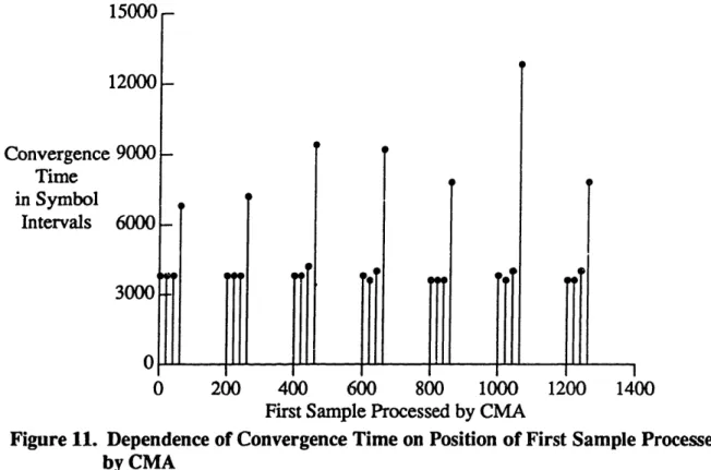
As mentioned above, there are four samples associated with each symbol. When the center tap is initialized to 1 and all other taps are set to zero, one of the four samples is effectively singled out as the sample that will be evaluated as the symbol. As shown in Figure 11, convergence time is affected by which of the four samples is chosen to be initially evaluated as the symbol.

I C/A/ 12000 Convergence 9000 Time in Symbol Intervals 6000 3000 0 T r UL I P 0 200 400 600 800 1000 1200 1400

First Sample Processed by CMA

Figure 11. Dependence of Convergence Time on Position of First Sample Processed by CMA

Figure 11 shows the convergence time of 28 runs of CMA using the same step size and input file.2 Four consecutive sample positions were studied at seven different locations

I 0 I _. I I 4 I I lm I I 4b _1 i I I I I : . . , I I ! I1 0 I I I I I

(38)

each separated by 200 samples. Convergence time was much longer for the fourth position than for the other three. Thus, convergence time clearly is affected by which sample is evaluated as the symbol. In many of the tests conducted for this research, convergence time was observed to depend on initial sample position.

This phenomenon is a natural result of the intersymbol interference introduced by pulse shaping. The Nyquist pulse is designed to introduce no intersymbol interference at the center of symbol intervals, but considerable intersymbol interference is introduced at the edge of symbol intervals. It is not known by the receiver which of the four samples is closest to the center of the symbol interval.

To help compensate for this problem, initializing the equalizer with two adjacent nonzero taps was explored. In some cases where a particularly bad initial sample would have been chosen, convergence time was reduced by as much as one half. However, in other cases performance was degraded. For the tests done in this section, the equalizers were initialized as mentioned in the previous subsection. However, since performance was recognized as dependent on the specific sample that was chosen as the symbol, a test of performance with CMA beginning at a particular sample was not done without also testing performance at three adjacent samples.

2. This graph describes performance of CMA with a real filter operating on data which has been processed by a Hilbert filter. The data file used was V29.4.4.hcn which was generated by a CODEX CCITT V.29 modem subjected to 100% envelope delay distortion. The step size used was 0.0024. Convergence time was measured using a threshold of 0.075.

(39)

5.5 CMA Structure Comparisons

The Codex LSI 96/V.29 modem transmitting a 16 point constellation under each of the eight channels discussed in Subsection 5.1 was used to compare performance of four implementations of CMA. The four implementations studied were 1) p= 2 with a complex equalizing filter and a preceding Hilbert filter, 2) p= 2 with a real equalizing filter and a preceding Hilbert filter, 3) p= 2 with a complex equalizing filter but no preceding Hilbert filter, and 4) p= 1 with a complex equalizing filter and preceding Hilbert filter.

The various structures and impairments were studied by performing equalization at sixty different initial sample positions at each of several step sizes. The sixty initial sample positions comprised four adjacent initial sample positions at 15 different locations sequentially separated by 2000 samples. There is a small sampling rate discrepancy introduced by nonidentical clocks used by the modems and the A/D converter. This discrepancy was utilized to insure that a range of initial sample alignments were studied by sequentially spacing the starting sample positions instead of randomly choosing them.

A mean minimum average error was obtained from each set of sixty minimum average errors. Mean convergence times were calculated in the same way. The two structures using p = 2 with a preceding Hilbert filter behaved almost identically in terms of mean minimum average error and mean convergence time. The structure which neglects the Hilbert filter and the structure which used p= 1 both showed poorer steady-state performance than the structures which used p= 2 with a preceding Hilbert filter.

(40)

Figures 12-15 plot mean minimum average error as a function of step size for the four structures being studied. Figure 12 shows the results for p =2 with a preceding Hilbert filter and a complex equalizer filter. Figure 13 shows the results for p=2 with a preceding Hilbert filter and a real equalizing filter. Performance is almost identical in these two graphs. As suggested in Section 4, when performing equalization in the passband, imaginary taps are completely unnecessary.

However, when complex taps are used, the imaginary taps do not remain low in power compared to the real taps. Since CMA is oblivious to output phase, an optimal equalizing filter multiplied by any complex constant of unity magnitude will also be optimal by the CMA criterion. CMA naturally adapts to a solution which uses all available taps instead of a solution which uses only half of them. The complex equalizer effectively uses twice as many real taps as the real equalizer. This explains why performance is identical when the step size used by the complex equalizer is half the step size used by the real equalizer.

As listed in Table 4, the threshold used to measure convergence time for the sixteen point V.29 constellation is 0.075. In both Figures 12 and 13, for step sizes near the center of the graph, the mean minimum average error is below 0.075 for all channels except for 100h _{percentile nonlinear distortion. A linear equalizer cannot be expected to compensate}

for severe nonlinearities. Severe nonlinear distortion remains an impediment to constellation identification. However, performance was acceptable for the 85'h percentile channel which contained nonlinear distortion, as well as the other five impairments being

(41)

n 1 v.1 0.09 -Mean 0.08-Minimum Average Error 0.070.06 0.05 -0.0005 85%o .-.0.. PLIU TUDE -rWITUD9 - ,-NOISE

.ml

O '''' . ,, - ....eo O EDi5 - -0.001 0.0015

CMA Step Size

0.002 Figure 12. Mean Minimum Average Error vs. Step Size for

Hilbert Filter and a Complex Equalizer Filter

Al U. -0.0025 p=2 with a Preceding 0.09 -Mean 0.08-Minimum Average Error 0.07-0.06 0.05. INW *L > .. AMPLITUDE -.-NOISE *·... E]:B .... _I...._..- _r

o-ED6w--

-I 0.003 CMA Step Size

Figure 13. Mean Minimum Average Error vs. Step Size for Hilbert Filter and a Real Equalizer Filter

p=2 with a Preceding .. . . 859to1 .... a Art .. rs . s @ ... ~~~~~~.... 0.001 0.002 0.004I 0.005 _ __ · · · 1 -LZ - _

(42)

studied, at the 85h percentile level. Actually, the 85" percentile channel contains no frequency offset since the 85h percentile level of this impairment is negligible.

Most of the curves in Figures 12 and 13 show mean minimum average error gradually increasing with step size. As step size increases, the adaptation resolution of the equalizer filter in the steady state will degrade. This results in a higher average error in the steady state. At some point, smaller step sizes will not improve the resolution of the filter. In fact, convergence will be slowed to the point that the steady state solution begins to degrade because dynamic behavior such as timing offset cannot be tracked. These points can be seen in Figures 12 and 13. For different impairments, the step size yielding the smallest mean minimum average error can be different.

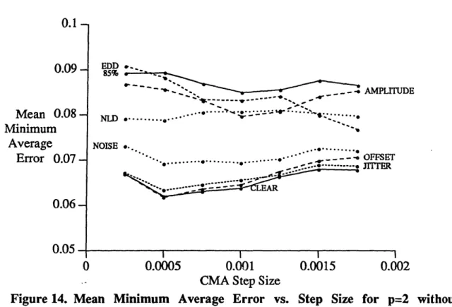
Figure 14 presents the results for p= 2 without a preceding Hilbert filter using a complex equalizer. For each impairment, the mean minimum average error is consistently higher than in the two previous figures. Performance was especially poor for the 100 percentile envelope delay distortion, nonlinear distortion, and amplitude distortion files, as well as the 85 percentile channel. For these cases the minimum average error was always higher than the 0.075 level.

From a computational perspective, it is not clear that neglecting the preceding Hilbert filter would be advantageous even if it were to perform as well as a receiver with the Hilbert filter. When the Hilbert filter is neglected, CMA must use complex taps. This replaces most of the computation avoided by neglecting the Hilbert filter. The Hilbert

(43)

nA V. I 0.09 -Mean 0.08-Minimum Average Error 0.070.06 0.05 -EDD '. 85% -- -...w- A. - , AMPLITUDE --- ,- " _ ND. ''- " ... -. ... NLD o....*. .... .

NOISE O.. 0* . .. ... F.E

* ~~'·

-- - - -* OFFSET

-. .. . .. . . .. . .. ... j . .

i; sk;==9LEA

0 0.0005 0.001 0.0015 0.002

CMA Step Size

Figure 14. Mean Minimum Average Error vs. Step Size for p=2 without a Preceding Hilbert Filter using a Complex Equalizer Filter

A V., 0.09 -Mean 0.08-Minimum Average Error 0.07-A Anf U.Uo-0.05 EDD *-.. . . 85% .9.U _* AMD ITT Tfl~s -'.. . --- ---'- . ".0. '_ NLD. .. NID · , c, ITnTeMD - ',. /" LEAR .. .. ''''''·''''' .- . · '' ,, -0 - - - -._~ _ 0 I; ET . ..-.- _A. I I 0 0.0002 0.0004 0.0006 0.0008 0.001

CMA Step Size

Figure 15. Mean Minimum Average Error vs. Step Size for p=l with a Preceding

Hilbert Filter using a Complex Equalizing Filter

rriER

-1 I · · -r

I I I I

~vlL

.7

(44)

filter does introduce additional delay. However, this delay (which is on the order of 10 msec), is negligible for the constellation identification application.

Figure 15 plots minimum average error versus step size for the fourth structure studied: p= 1 with a complex equalizing filter and a preceding Hilbert filter. This structure did not perform as well as the first two structures discussed. Three channels never achieved a mean minimum average error of 0.075: 100h percentile envelope delay distortion, 100hpercentile amplitude distortion, and the 85hpercentile channel.

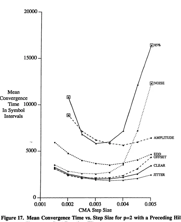
From Figures 12-15 it is clear that p= 2 with a preceding Hilbert filter is superior to alternatives for the conditions studied. Convergence time was studied for seven of the eight channels to explore whether the real filter adapted more or less quickly than the complex filter. Nonlinear distortion was not studied for convergence time because it did not consistently achieve a minimum average error below the threshold used to measure convergence time (0.075). Figures 16 and 17 plot mean convergence time versus step size for a complex equalizing filter and a real equalizing filter respectively. Once again there is almost no difference in performance between a real and a complex equalizer filter.

Different channels had mean minimum convergence times at different step sizes. However, in both figures there is a step size for which all channels had a reasonably small mean convergence time of around 6000 samples. Increasing step size decreases convergence time until the step size is large enough that the individual filter updates are

(45)

weighted more heavily than their accuracy dictates. For the case of additive noise it is not surprising that the decrease in convergence occurs at a smaller step size and more abruptly than with the other impairments. Additive noise is not removed as easily by a linear equalizer filter because it is not a linear impairment.

Figures 10-17 all indicate similar performance for the 100 percentile channels with impairments of frequency offset and phase jitter, and the clear channel. The CMA objective function given in Eq. (2) contains only the magnitude of the output symbol. The impairments of frequency offset and phase jitter only affect the symbol phase. Thus these impairments are invisible to CMA.

(46)

15000 Mean Convergence Time 10000 In Symbol Intervals 5000 0 JNOISE i- AMPLITUDE , EDD . OFFSET . CLEAR 0. . JIrrTER 0.0005 0.001 0.0015 0.002 CMA Step Size

Structure 1

Figure 16. Mean Convergence Time vs. Step Size for p=2 Filter and a Complex Equalizer Filter

0.0025

with a Preceding Hilbert

(47)

"} '/n /~V%/VVv15000 -Mean Convergence Time 10000-In Symbol Intervals ,. 5000

-

0-85% NOISE AMPLITUDE Sr - -V ·. ' ,, EDD -' * OFFSET

",'/

CLEAR

-- *. ... .... . .. n A T --- 0 ER·.-- .JTER ... ... i" ' " I -I I I I 0.001 0.002 0.003 0.004 0.005

CMA Step Size

Figure 17. Mean Convergence Time vs. Step Size for p=2 with a Preceding Hilbert Filter and a Real Equalizer Filter

(48)

Some insight into the differences between the three structures employing p = 2 CMA can be gained by exploring the frequency domain representation of the equalizer filters obtained by CMA after the convergence threshold of 0.075 has been crossed. Figure 18 shows the frequency domain representation

Magnitude 2 1 3.14 1.57 Phase in 0 Radians -1.57 -3_14 Figure 18. '- '- I I I I I -4800 -2400 0 2400 4800 Hertz

Frequency Domain Representation of the Equalizer Filter Arrived at after 6000 Symbols by CMA Without a Preceding Hilbert Filter Using a Complex Equalizing Filter. A Constant Delay of 48 Samples Has Been Removed from the Phase Response.

of the equalizer filter obtained after 6000 symbols processing a signal transmitted over a clear channel using CMA without a preceding Hilbert filter. The magnitude response shows that negative frequencies from -300 Hz to -3300 Hz are being severely attenuated. Thus the equalizing filter is performing the function of the neglected Hilbert filter. Phase

t-

--

·

I r 0I 11 1

(49)

was set to zero in the region of severe attenuation because phase becomes erratic as magnitude approaches zero.

The observed gain of 2.8 in the passband of the filter is as expected. The input signal had an RMS value of .5 and thus a power of 0.25. Half of this power was removed by the equalizing filter, leaving 0.125. To increase the power to 1 a gain of about 2.8 is necessary.1

Figures 19 and 20 present the frequency domain representation of the equalizer filter obtained after 6000 symbols of processing by CMA using complex taps and real taps respectively. In both cases a preceding Hilbert filter was used. Both cases resulted from processing the same clear channel data file processed for Figure 18. The observed passband gain of 1.4 is expected since the input signal after Hilbert filtering has a power of 0.5 and the output signal needs to have a power of one to agree with the value chosen

for R2

Figure 19 shows that when the complex tap filter is used with a preceding Hilbert filter, the magnitude and phase responses for negative frequencies remain virtually the same as the unity magnitude response and flat phase response of the initial tap setting.

1. Figures 18 19, and 20 all resulted from processing a sampled 16 point V.29 constellation transmitted over a clear channel by the Codex LSI 96/V.29 modem used in earlier tests. In all three cases processing started with the first sample in the data file. Figure 18 used a step size of 0.0015 with complex taps but no Hilbert filter. The average error computed for the window following symbol 6000 was 0.0738. Figure 19 resulted from using a step size of 0.0015 with complex taps and a preceding Hilbert filter. The average error computed for the window following symbol 6000 was 0.0750. Figure 20 resulted from using a step size of 0.003 with real taps and a preceding Hilbert filter. The average error calculated for the window following symbol 6000 was 0.074 1.

(50)

The Hilbert filter removed the input signal power for negative frequencies. Thus, there was no energy present to drive filter adaptation at negative frequencies. Figure 20 demonstrates the conjugate symmetry all real filters must have. The response shown in Figure 19 and the response shown in Figure 20 are similar for positive frequencies. This is consistent with the similar convergence behavior displayed by p = 2 CMA with real or complex taps.

(51)

2-Magnitude

1-

f-1 A Phase in Radians D. JI 1.57 -0 1.57 - -3.14--4800 -2400I I 0 Hertz 2400 4800

Figure 19. Frequency Domain Representation of the Equalizing Filter Arrived at by CMA after 6000 Symbols Using a Complex Equalizing Filter. A Contant Delay of 48 Samples Has Been Removed from the Phase Response.

3-

2-Magnitude

1- 0-' IA Phase in Radians 3. 1q' 1.57

-

01.57 -_ A -4800 -2400I I 0 Hertz I 2400 4800

Figure 20. Frequency Domain Representation of the Equalizing Filter Arrived at by CMA after 6000 Symbols Using a Real Equalizing Filter. A Contant Delay of 48 Samples Has Been Removed from the Phase Response.

_____ ______ ____Y_______I __ _· · w - - - -'1 ---_ , . IlJ all

(52)

CMA could be used alone in a constellation identification scheme, or performance might be improved by eventually switching to magnitude decision direction as discussed in the following section. In either case, computational complexity would be minimized if one blind equalizer could remove channel impairments regardless of the constellation being transmitted. One set of CMA parameters must work for all constellations for this to be the case.

The two parameters of CMA which might depend on the constellation are R2and the

adaptation step size a These parameters were introduced in Section 4. As shown in Table 2, the values of R2vary from 1.000 to 1.418 when the constellation magnitudes are

normalized to have an RMS value of one. Within this range of values, using one value of

R2 for all the constellations will merely cause the outputs for various constellations to be

scaled. The previous study showed empirically that p=2 CMA can converge when faced with an input signal requiring a gain of 1.4. The scaling required to allow the use of one

R2 for all constellations will be less than 1.4. Constellation dependent scaling will not

interfere with identification since the scale factor is easily calculated by the following equation:

scale factor = (20)

A study was performed for p=2 CMA with real taps and a preceding Hilbert filter which revealed that one step size yields acceptable performance with respect to convergence time and minimum average error for all constellations being studied. This

(53)

study assessed mean minimum average error and mean convergence time as a function of step size for the nine signals listed in Table 2 transmitting over the channel containing all six impairments at the 85' percentile level. This channel was used because it was found in the previous subsection (see Figure 16) to be the most sensitive to step size of the seven channels which CMA successfully received. For each constellation at each step size, equalization was performed at twenty different sample positions comprising four adjacent sample positions at five different locations. The five locations were sequentially spaced by 6000 samples.

Figure 21 shows mean minimum average error as a function of step size for eight of nine the signals studied. For a step size of 0.003, all eight signals achieved a mean minimum average error which is below their respective thresholds used for measuring convergence as listed in Table 4. However, this was not always the best possible step size.

The curves associated with V.33, nine and sixteen magnitude constellations, are flat. The nine magnitude constellation achieved a mean minimum average error of about 0.04 regardless of step size, and the sixteen magnitude constellation achieved a mean minimum average error of about 0.02 regardless of step size. Referring back to Figure 10 reveals that the values of mean minimum average error achieved by these two constellations are in the flat regions of their respective observed average error versus ideal average error curves. Unfortunately, these two constellations have magnitudes so closely spaced that the average error criterion is useless as a measure of ultimate