HAL Id: hal-01856121
https://hal.archives-ouvertes.fr/hal-01856121
Submitted on 4 Sep 2020
HAL is a multi-disciplinary open access
archive for the deposit and dissemination of
sci-entific research documents, whether they are
pub-lished or not. The documents may come from
teaching and research institutions in France or
abroad, or from public or private research centers.
L’archive ouverte pluridisciplinaire HAL, est
destinée au dépôt et à la diffusion de documents
scientifiques de niveau recherche, publiés ou non,
émanant des établissements d’enseignement et de
recherche français ou étrangers, des laboratoires
publics ou privés.
Distributed under a Creative Commons Attribution - NonCommercial - NoDerivatives| 4.0
International License
Virgile Rakoto, Philippe Lognonné, Lucie Rolland, P. Coisson
To cite this version:
Virgile Rakoto, Philippe Lognonné, Lucie Rolland, P. Coisson. Tsunami Wave Height Estimation
from GPS-Derived Ionospheric Data. Journal of Geophysical Research Space Physics, American
Geo-physical Union/Wiley, 2018, 123 (5), pp.4329 - 4348. �10.1002/2017JA024654�. �hal-01856121�
Tsunami Wave Height Estimation from GPS-Derived
Ionospheric Data
Virgile Rakoto1 , Philippe Lognonné1 , Lucie Rolland2, and P. Coïsson1
1Institut de Physique du Globe de Paris-Sorbonne Paris Cité, Université Paris Diderot, Paris, France,2Université Côte d’
Azur, OCA, CNRS, IRD, Géoazur, Valbonne, France
Abstract
Large underwater earthquakes (Mw> 7) can transmit part of their energy to the surrounding ocean through large seafloor motions, generating tsunamis that propagate over long distances. The forcing effect of tsunami waves on the atmosphere generates internal gravity waves that, when they reach the upper atmosphere, produce ionospheric perturbations. These perturbations are frequently observed in the total electron content (TEC) measured by multifrequency Global Navigation Satellite Systems (GNSS) such as GPS, GLONASS, and, in the future, Galileo. This paper describes the first inversion of the variation in sea level derived from GPS TEC data. We used a least squares inversion through a normal-mode summation modeling. This technique was applied to three tsunamis in far field associated to the 2012 Haida Gwaii, 2006 Kuril Islands, and 2011 Tohoku events and for Tohoku also in close field. With the exception of the Tohoku far-field case, for which the tsunami reconstruction by the TEC inversion is less efficient due to the ionospheric noise background associated to geomagnetic storm, which occurred on the earthquake day, we show that the peak-to-peak amplitude of the sea level variation inverted by this method can be compared to the tsunami wave height measured by a DART buoy with an error of less than 20%. This demonstrates that the inversion of TEC data with a tsunami normal-mode summation approach is able to estimate quite accurately the amplitude and waveform of the first tsunami arrival.1. Introduction
Tsunamis are long-period oceanic gravity waves mostly generated by earthquakes or landslides (Satake, 2002). They propagate with a velocity of 200–300 m/s depending on the water depth, and their wave height is amplified when approaching the coast, leading to disastrous flooding when large. The deadliest tsunami ever recorded in human history was triggered by the Sumatra-Andaman earthquake (Mw = 9.3, e.g., Stein & Okal, 2007), which occurred on 26 December 2004. Tsunamigenic earthquakes have also occurred in sev-eral other regions of the Pacific Ocean, including Valdivia, Chile in 1960; Papua New Guinea in 1998; the Kuril Islands in 2006 and 2007; the Solomon and Santa Cruz Islands in 2007 and 2013; Samoa in 2009; Chile in 2010 and 2014; and Japan, whose Tohoku-Oki event in 2011 was one of the costliest tsunami disasters (more than 220 billion USD).
All these events have stimulated both research and infrastructure development with the goal of improving the detection and monitoring of tsunamis, so as to be able to warn authorities and populations likely to be affected. Thus, the tsunami monitoring effort, which was at first exclusively focused on the Pacific area, expanded rapidly toward worldwide coverage by tsunami real-time warning systems (Titov et al., 2005). See National Research Council (2011) for a general report on the US Tsunami Warning System.
The Tsunami Early Warning System includes the DART (Deep-ocean Assessment and Reporting of Tsunamis) system of buoys, which is the most effective tool for assessing by measurements the predicted amplitude of a tsunami once triggered by an earthquake. This system can provide in real time an accurate measurement of the tsunami wave amplitude (with a 3 cm detection threshold in the North Pacific area) in the open ocean despite the waves long horizontal length (up to 200 km) and small amplitude.
However, a dense detection and monitoring system for tsunamis in the open ocean remains costly, as DART buoys are complex to install and require frequent maintenance. Complementary measurements could also be useful to back up the DART buoys when they are temporarily down in critical areas at the time of the tsunami wave arrival.
RESEARCH ARTICLE
10.1002/2017JA024654 Key Points:
• Inversion of the perturbed TEC induced by three tsunamis was performed to estimate their maximum
• We estimated that the error in the tsunami height of three events was less than 20
• The inversion success can be limited ionospheric condition Correspondence to: V. Rakoto, [email protected] Citation: Rakoto, V., Lognonné, P., Rolland, L., & Coïsson, P. (2018). Tsunami wave height estimation from GPS-derived ionospheric data.
Journal of Geophysical Research: Space Physics, 123, 4329–4348.
https://doi.org/10.1002/2017JA024654
Received 4 AUG 2017 Accepted 23 JAN 2018
Accepted article online 30 JAN 2018 Published online 28 MAY 2018
©2018. The Authors.
This is an open access article under the terms of the Creative Commons Attribution-NonCommercial-NoDerivs License, which permits use and distribution in any medium, provided the original work is properly cited, the use is non-commercial and no modifications or adaptations are made.
The use of ionospheric signals measured by Global Navigation Satellite Systems (GNSS) (Artru et al., 2005; Kamogawa et al., 2016; Occhipinti et al., 2008; Rolland et al., 2010) has therefore been proposed in many papers as a means of completing and improving tsunami warning systems, from the early proposals of Hines (1972) and Peltier and Hines (1976) to a first patent proposing to extract the total electron content (TEC) from dual-frequency satellite systems (MacDoran, 1981) and finally to the most recent research papers (Kamogawa et al., 2016; Savastano et al., 2017). However, none of these works have demonstrated that TEC signals could be used to reproduce the signals recorded by the DART buoys with an accuracy compliant with that required for warning systems.
Let us first go back to the early proposals made in the 1970s. Hines (1972) and Peltier and Hines (1976) first suggested that earthquakes, tsunamis, or volcanic eruptions generate internal gravity waves (IGWs), which propagate from the bottom to the top of the atmosphere. When these waves reach the ionosphere, they interact with the plasma and produce a detectable signal (e.g., TEC, airglow) in ionosphere.
Even if the amplitude of the tsunami is small compared to the ocean swell, it can generate IGWs due to its long wavelength. As the kinetic energy is conserved up to an altitude of about 200 km, and air density decreases exponentially with altitude, the IGWs are then strongly amplified in the atmosphere. The ratio of the amplitude of the velocity wave between the ionospheric height and the ground level is about 104–105.
The ionospheric perturbations induced by a tsunami were observed for the first time in GNSS-derived TEC signals by Artru et al. (2005) off Japan using the dense Japanese GEONET network. The Peru, 23 June 2001
MW = 8.2 earthquake triggered a tsunami which reached the Japanese coast about 22 h after the rup-ture. At the same time, a clear TEC perturbation of about 1 TECU was recorded. In addition, the direction of propagation of the TEC perturbation (slightly southwestward) was consistent with that of the tsunami. After the giant Sumatra Andaman tsunami, similar signals were identified by Liu et al. (2006) using GPS data from ground-based stations in the Indian Ocean area. The TEC measurements derived from the JASON-1 and Topex/Poseidon satellite altimetry data were reconstructed by Occhipinti et al. (2006) using a tsunami wave-field as input for a coupling model. Rolland et al. (2010) also detected and analyzed the ionospheric signature of three transpacific tsunamis off Hawaii generated by the 2006 Kuril Islands earthquake (Mw= 8.3), the 2009 Samoa earthquake (MW = 8.1) and the 2010 Maule earthquake (MW = 8.8), the latter two also reported by Galvan et al. (2011). The ionospheric signature in TEC was in that case compared to the tsunami height mea-sured by the functioning buoy the closest to Hawaii: DART buoy 51407 (50 km west of Hawaii) in the case of the Kuril event and 51406 (5370 km southeast of Hawaii) in the case of the Samoa event. Unfortunately, neither of these two DART buoys was working at the arrival time of the Chilean event in Hawaii. For all these events, the IGW propagation speed and direction were consistent with those of the tsunami, and the TEC perturba-tion and tsunami height had a similar waveform, with a consistent delay between the two signals (±13 min). A similar TEC signal was later detected in the case of the tsunami triggered by the Mw = 9.0 Tohoku event in 2011 (Galvan et al., 2011; Kherani et al., 2016; Rolland, Lognonné, Astafyeva, et al., 2011), including from TEC radio occultation performed by COSMIC (Coïsson et al., 2015), and by the more recent 2012 Haida Gwaii tsunami (Grawe & Makela, 2015; Savastano et al., 2017), the Chilean event of 2014 (Zhang & Tang, 2015) and the 2015 Illapel tsunami (Grawe & Makela, 2017).
All these observations were first a challenge to modeling and more recently to inversion efforts. Early mod-els (Occhipinti et al., 2006, 2011) were produced by considering the simplified case of noncompressible and nonattenuated gravity waves and by exciting these waves with the simulated 2-D height variation in sea level. Although the general shape of the waves was retrieved, these simplifications led to unrealistically large IGW amplitudes, with vertical and horizontal winds of about 600 m/s. The attenuation of gravity waves in the upper atmosphere, included by Hickey et al. (2009) and Mai and Kiang (2009), must be taken into account. These first modeling results were rapidly followed by more comprehensive wave propagation mod-els taking into account electromagnetic field perturbations, viscosity, and compressibility (Kherani et al., 2012, 2016). Other numerical approaches based on fully nonlinear modeling of thermospheric coupling effects (Meng et al., 2015), the wave packets modeling technique (Vadas et al., 2015) or the perturbation theory of acoustic-gravity waves (Godin et al., 2015) were also developed. Last but not least, Coïsson et al. (2015) pre-sented the normal-mode summation technique, which is based on the computation of tsunami normal modes for Earth models integrating the solid, oceanic, and atmospheric domains as well as gravity, compressibil-ity, and viscosity of the atmosphere, in ways similar to the computation of Rayleigh normal modes for Earth (Artru et al., 2001, 2004; Lognonné et al., 1998; Rolland, Lognonné, Munekane, et al., 2011) and other planets
(Lognonné et al., 2016). The summation of tsunami normal modes was able to model TEC data quite accu-rately, with a 20% error when modeling the amplitude waveform using a finite source model of the Tohoku earthquake source. This forward modeling, which has been detailed by Rakoto et al. (2017), will be the one used in the inversion strategy developed in this paper.
This paper first presents the authors TEC perturbation and tsunami height observation method. It then briefly recalls the forward modeling of these two quantities using normal mode summation, and describes the inver-sion method. Using the GPS-TEC data of the 2012 Haida Gwaii tsunami in far field, the 2006 Kuril tsunami (far field), and the 2011 Tohoku tsunami (both in near field and far field), we then show the results of the inversion of the arrival of the tsunami first wave packet, and compare it to DART observations. We finally discuss the reliability of the inversion in terms of amplitude errors, the selection of GPS-TEC data, ionospheric conditions and limitations, and finally future prospects.
2. Theory and Models
2.1. Forward Modeling
Most of the models of TEC perturbations induced by tsunamis are based on the excitation of atmospheric gravity waves by the vertical displacement of the oceans surface, through the continuity boundary condi-tion of this vertical displacement and by the further interaccondi-tions of the generated gravity waves with the ionospheric plasma (Kherani et al., 2012, 2016; Meng et al., 2015; Occhipinti et al., 2006, 2008, 2011; Vadas et al., 2015).
Tsunami waveforms, like all other waves propagating on Earth, can be computed by normal-mode summation (Okal, 1982; Ward, 1980). The excitation of each normal mode is furthermore directly related to the seismic source either through a single, point source, Centroid Moment Tensor (CMT, e.g., Dziewonski et al, 1981) or through a series of CMTs at multiple location (for finite source models). This was the approach proposed by Coïsson et al. (2015): the tsunami normal modes were computed with their coupled counterpart in the atmo-sphere in accordance with the formalism developed by Lognonné et al. (1998), which considers all boundary conditions and implicitly takes into account the full coupling between the solid Earth, ocean, and atmosphere (Lognonné et al., 1998; Watada et al., 2014), as well as atmospheric viscosity (Artru et al., 2001; Lognonné et al., 2016). However, we neglected the background atmospheric neutral wind that causes a nonzero advection term in the normal mode equation. This term can be written in the following form:(v0⋅ 𝛁
)
v ∝𝜔vv0∕ctsunami with𝜔 the normal modes eigenfrequency, and ctsunami≈ 220 m s−1. Therefore, up to background neutral wind about 30 m s−1, the advection term can be neglected compared to𝜕v∕𝜕t ∝ 𝜔v, although large effects can of course be observed for winds of 100 m/s and along wind propagation path as shown by Hickey et al. (2009). Furthermore, the normal modes approach may also be used to calculate displacement in the oceanic part; displacement or strain in the solid part; and wind, adiabatic temperature, and density variations in the atmospheric part.
In this paper, we use the classical representation of the seismic source of the CMT, popularized by the CMT project in long period seismology (Dziewonski et al., 1981). The excitation of the Earth’s normal modes by a seismic event is therefore modeled by a CMT source applied to a point source (Phinney & Burridge, 1973) located at r0. When the source time function is a simple Heavyside function H(t), the displacement induced by a tsunami uDC(r, r0, t) at any location r for a spherical coordinate system is then expressed as (Lognonné, 1991)
uDC(r, r0, t) = H(t)Re ∑ k≥0 [ M ∶𝝐k(r0) 1 − ei𝜎kt 𝜎2 k uk(r) ] , (1)
where t is the time, Re the real part, M is the moment tensor,𝝐kthe strain at the source location r0associated with the complex eigenfunction uk, and the eigenfrequency𝜎k. Positive index k denotes a normal mode sin-glet with positive real part frequency and therefore the three quantum numbers:𝓁, m, n for the azimuthal, longitudinal, and radial numbers, respectively.
For a spherically symmetric Earth, the amplitude of normal modes uk(r) is proportional to spherical harmon-ics, and the equation above can be rewritten in new spherical coordinates locating the source at the pole in the form: uDC(r, t) = Re ∑ 1≤p≤6 mp ∑ K,|m|≤2 Ψp,mK (r0) umK(t), (2)
where the normal mode response uK,m(t) is given by uK,m(t) = H(t)1 − ei𝜎K t 𝜎2 K umK(Δ, 𝜙) (3)
and where Δ and𝜙 are the great circle distance and azimuth between the source and location; r, mpare the six independent components of symmetric tensor M noted now in vector form as m = [Mrr, Mr𝜃, Mr𝜙, M𝜃𝜃, M𝜙𝜙, M𝜃𝜙]. Ψp,mK are functions depending on the strain tensor components of the mode K expressed at the radius of the source r0. More details can be found in Phinney and Burridge (1973), together with expressions of the Ψp,mk terms. Note here that the summation involves K numbering multiplets, and therefore depends only on the two quantum numbers𝓁 and n. Only singlets with |m| ≤ 2 are summed for a double couple source. The tsunami modes of the whole solid Earth-ocean-atmosphere system are one branch of spheroidal nor-mal modes, corresponding to gravity modes of the oceanic layer. They are computed in accordance with Coïsson et al. (2015) and Rakoto et al. (2017) between𝓁 = 40 and 𝓁 = 520, which corresponds to the 0.2 mHz to 2.6 mHz frequency range. The Earth’s internal structure model, needed for the computation, is provided by the Preliminary Reference Earth Model (Dziewonski & Anderson, 1981) with an ocean depth set to the average over the region located below the sounded area. The value of the ocean depth is obtained from the General Bathymetric Chart of the Oceans. The surrounding atmosphere and its structure are modeled by the NRLMSISE-00 empirical model (Picone et al., 2002), taken on the day and at the local time of the observa-tion. Despite its potential effect on TEC amplitudes, especially for eastward propagation path (Hickey et al., 2009), we did not introduce yet in our approach the wind effects from empirical models (Drob et al., 2015) and will discuss further the associated consequences in the Discussion section.
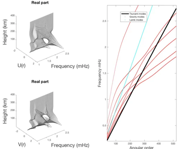
Figure 1 shows the real part of the vertical (U(r)) and horizontal (V(r)) eigenfunctions in the atmosphere and the dispersion diagram of the tsunami normal modes computed for the Haida Gwaii event. The tsunami branch crosses one of the gravity branches at 1.5 mHz, 2.0 mHz ,and 2.5 mHz. Thus, and at these frequen-cies, resonance will occur and the vertical and horizontal components (U(r) and V(r)) of tsunami normal mode eigenfunctions will be large.
The amplitudes obtained with equation (2) are then convolved with time source function fdtc,𝜏(t). This time source function is represented by a rectangle function whose half width is equal to half the source dura-tion𝜏 and delayed by a time shift dtc. For finite source models, this process is repeated for each patch of the source, and the final amplitude is then obtained by summing the contributions of all the patches. The source parameters used to forward model the three studied events are taken from the USGS website (http://earthquake.usgs.gov/ (Hayes, 2011)) for each of the three studied events.
We first model the neutral velocity field in all three directions (vertical, south, and east) directly from equation (2) which will finally have 31 (locations) ×3 (axes) time. For each of these time series, a neutral atmosphere/ionosphere coupling is performed.
Ion velocity viis expressed as (Macleod, 1966) vi= 1 1 +𝜅2 [ 𝜅2(V × 1 b) × 1b+𝜅V × 1b+ (1 +𝜅2)(V⋅ 1b)1b ] , (4)
with 1bthe geomagnetic field unit vector,𝜅 the ratio of the neutral ion collision frequency with gyrofrequency
𝛾i = qiB∕mi, where B is the magnetic field intensity, qithe ion charge, and miits mass. As the ion-neutral collision frequency decreases at high altitudes,𝜅 was neglected in the F region and equation (4) thus becomes (Hooke, 1970) vi= ( v⋅ 1b ) 1b. (5)
Therefore, the modeling only takes into account the dynamics along the magnetic field. However, this approx-imation has some limitations in the ionosphere since the perpendicular dynamics causes also density changes (Chum et al., 2016). Future investigations might account the full terms to improve both the modeling and associated inversions.
The electron density fluctuations are obtained from the continuity equations for the ions:
𝜕ne
𝜕t +𝛁 ⋅
(
Figure 1. Normal mode characteristics. (left) Amplitude of the atmospheric part of vertical (Ur) and horizontal (Vr)
normal mode eigenfunctions, scaled by the square root of density. (right) Dispersion of normal modes for the full Earth system from 0.2 mHz to 2.6 mHz. Tsunami modes are plotted in black, atmospheric gravity modes in red, and Lamb modes in light blue.
where ne is the electron density and where we neglect recombination and production processes in the frequency bandwidth concerned by tsunami signals. Assuming only small fluctuations, we can linearize:
ne= n0e+𝛿ne, where n0eis the ionosphere steady state electron density and𝛿nethe perturbation generated by the tsunami waves. After integration, the continuity equation becomes
𝛿ne= −𝛁 ⋅ (
n0eui )
, (7)
with uithe displacement of the ions. Contrary to previous modeling approaches (Coïsson et al., 2015; Rolland, Lognonné, Munekane, et al., 2011), equation (7) is not computed with a grid but directly with an analyti-cal solution using the normal-mode formalism (Phinney & Burridge, 1973), which may be used to compute the divergence of angular order𝓁 for normal modes and project it on the magnetic field. The unperturbed ionospheric electron density (n0
e) and geomagnetic field are computed at the location and time of the tsunami arrival at the receiver using the International Reference Ionosphere (Bilitza & Reinisch, 2008) and the International Geomagnetic Reference Field (Maus et al., 2005), respectively.
It should be noted that, as the lateral mean electron density profile is smooth, the profile of the mean electron density n0
eis computed at the average ionospheric pierce point (IPP) location for each altitude. However, there was no approximation when calculating the magnetic field. The last step in the forward problem involves computing the TEC by integrating the electron density along path ds between the ground receiver and the GPS: TEC(t) = ∫ Satellite(t) Receiver ne ( rs, t ) ds(t), (8)
where rsis the position along the integrated ray path. We recall that the location of the satellite, and there-fore the integration path is depending on the time. The relations (3) to (7) are all linear and can therethere-fore be computed either for the full seismogram or for each individual contribution to the normal modes. This means that TECDC(t) = Re ∑ 1≤p≤6 mp ∑ K,|m|≤2 Ψp,mK (r0) TECmK(t), (9) where TECDCdenotes the modeled TEC with a double couple source and TECK(t) the TEC response of the tsunami multiplet (K, m). Both fields depend on the epicentral distance, azimuth, satellite-station pair, and local time, in the latter case through the electron density profile of the ionosphere, n0. These dependencies will be considered as implicit.
2.2. Inversion
When comparing equations (2) and (9), it may be noted that the CMT parameter Mpmay be used to compute the TEC, the neutral wind, the ocean surface perturbation, or the surface acceleration. For surface acceleration, this is the theoretical ground for all CMT inversions, either based on Network (e.g., Dziewonski et al., 1981) or on single station (e.g., Fan & Wallace, 1991; Kim et al., 2000; Walter, 1993). Its extension to TEC and ocean surface perturbation is the key point in our inversion process, during which we use the TEC data to invert the best Mpparameters, thus allowing us to immediately reconstruct either the neutral wind or the ocean surface displacement. Let us therefore assume that locally the observed tsunami wavefront can be approximated by the wavefront generated by a local double couple seismic source located at the epicenter, which means that
u(r, t) = H(t)Re ∑ 1≤p≤6 mlocal p 𝜕uDC(t) 𝜕mp , (10) TEC(t) = H(t)Re ∑ 1≤p≤6 mlocalp 𝜕TECDC(t) 𝜕mp , (11)
where the two partial derivatives are given by
𝜕uDC(t) 𝜕mp = ∑ K,|m|≤2 Ψp,mK (r0)1 − ei𝜎K t 𝜎2 K umK(Δ, 𝜙) , (12) 𝜕TECDC(t) 𝜕mp = ∑ K,|m|≤2 Ψp,mK (r0) TECmK(t). (13)
The main difference between this local model of the waveforms and the CMT model lies in the moment ten-sor’s six parameters, which may depend on the position and azimuth, in order to integrate the source radiation pattern as well as all 3-D effects on the waveform. In order to better match the observation, we add a source function term, which provides our final forward model expression for TEC:
TEC(t) = Re ∑ 1≤p≤6
mlocalp 𝜕TECDC(t)
𝜕mp
∗ fdtc,𝜏(t), (14)
where the asterisk (∗) denotes the convolution product. To summarize, the inversion is designed to invert from the TEC data set the best eight local source parameters given by moment tensor component m, the time shift, dtc, and the temporal half duration of the source, (𝜏).
This inversion is performed by a least squares method by minimizing the cost function between the model and data:
C(dtc, m) = ∫
t2 t1
[
TEC(t,dtc, m) − TECobs(t)]2
𝜎2 dt, (15)
where TECobs(t) is the observed GNSS TEC time series and t1, t2are the start and end time of the record selected for inversion. The TEC noise measurement error estimation, denoted𝜎, is then estimated from the TEC RMS amplitude 1 day before the tsunami is detected. This typically corresponds to the ionospheric variability in the bandwidth chosen for TEC signal filtering. The inversion is linear with respect to the local moment tensor components but nonlinear with respect to the source function due to the fact it is set by local time shift (dtc) and half source duration (𝜏). As the typical value of the half source duration 𝜏 ≈ 10−80 s is much smaller than
the dominant period in the TEC perturbation signal T ≈ 667 s (with a corresponding frequency of 1.5 mHz), the TEC perturbation (and the tsunami height) is not very sensitive to the half source duration. We therefore do not invert it and instead use the value provided by the seismic CMT inversion. Local time shift dtc is, on the contrary, very sensitive to the delay in propagation associated with bathymetric variations occurring along the whole length of tsunami propagation. Therefore, dtc is inverted through a grid search between −1 h and +1 h with respect to the seismic CMT value and with a scanning step corresponding to the 30 s sampling rate of the TEC data. For each step, the moment tensor is then inverted with the linear least squares method and the cost function computed. This moment tensor inversion is based on the solving of the linear system:
6 ∑ i=1 Aijmj= Bj, (16) with Akk′= ∫ t2 t1 [𝜕TEC DC(t) 𝜕mk ∗ fdtc,𝜏(t) ] [𝜕TEC DC(t) 𝜕m′ k ∗ fdtc,𝜏(t) ] dt, (17) Bk= ∫ t2 t1 [𝜕TEC DC(t) 𝜕mk ∗ fdtc,𝜏(t) ] TECObs(t) dt. (18)
As only vertical motions excite a tsunami, pure strike-slip moment tensor components cannot be inverted, nor any source mechanism generating small tsunami signals. We manage this inversion by performing a singular value decomposition of our inversion problem, detailed in Appendix A. After each local moment tensor inver-sion for a given dtc, the misfit between the observed and the modeled TEC is computed. The final solution is the one that minimizes the cost function.
In order to model the extension of the source, we also performed inversion with two point sources. The param-eters related to this second source are noted with a prime (′) symbol. This source is also located at the epicenter but has a higher initial time shift (dtc′i) which represents the extension of the source.
3. GNSS-Derived and DART Data
We used the freely available 30 s GPS raw data from the UNAVCO website (http://www.unavco.org). The TEC is extracted from the measurement of the two carrier frequencies (f1= 1,575.42 MHz and f2= 1,227.60 MHz). We computed the biased slant TEC using the L1and L2carrier phase difference for each satellite-ground base station pair in accordance with Lognonné et al. (2006) and Mannucci et al. (1998). The long-period signal due to daily ionospheric variations, satellite motion, and near-constant instrumental noise is removed through a polynomial fit of order 10. The data are then filtered with a third-order Butterworth filter (between 0.2 mHz and 2.6 mHz for Haida Gwaii and Tohoku, and between 1 mHz and 2.6 mHz for Kuril) to emphasize the IGW component of the signal. The perturbed TEC signal for both the day of the earthquake and the following day was computed in order to ensure that the observed perturbation is indeed related to the propagation of IGWs. TEC error𝜎 was also measured from these two data sets.
For each satellite-ground base receiver pair, the observed data are associated with a single IPP. The IPP, mov-ing over time in keepmov-ing with the GPS satellite, is defined as the intersection of the satellite-receiver line of sight with a thin shell located at the maximum altitude of the F2ionospheric peak (thin layer approximation). However, this thin layer approximation is only used to describe the TEC measurement and is not used in our modeling. Therefore, the first step of the forward modeling consist in computing the 31 IPP positions for a given GPS satellite-station pair between 100 and 400 km every 10 km with a 30 s time step. Then the pertur-bation of electron density is recomputed at every time step in order to model the TEC perturpertur-bation following the method explained in section 2.1.
Each DART buoy system consists of an anchored surface buoy with a bottom pressure recording sensor. The buoy receives the measurements of the bottom pressure recording sensor (which are subsequently con-verted into water height) via an acoustic transmission. In order to compute the tsunami height, the raw data were detided. The tides were modeled with a polynomial fit (Watada et al., 2014). The time series was then band-pass filtered with the same third-order Butterworth filter as the TEC data.
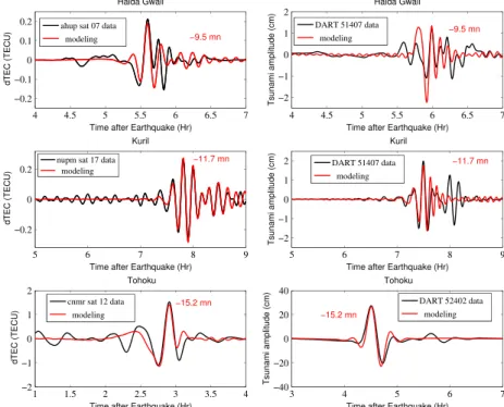
Figure 2. Comparison between data (black) and modeling (red) for the TEC (left panels) and tsunami height (right
panels) in the case of Haida Gwaii, Kuril, and Tohoku events. The real and the modeled data were filtered between 0.2 mHz and 2.6 mHz for Haida Gwaii and Tohoku, and between 1 mHz and 2.6 mHz for Kuril. Note that the GPS station and the DART buoy for Tohuku are not colocated, whereas those for Kuril and Haida Gwai are much closer together.
4. Results
4.1. Case Studies
In this paper, we studied three tsunami events: the 2012 Haida Gwaii and 2006 Kuril Islands earthquakes and the 2011 Tohoku tsunami. The 2012 Haida Gwaii and the 2011 Tohoku event received great attention in the past literature and are often used as test case. The choice of analyzing 2006 Kuril event over the Chile 2010 or 2015 was motivated by the fact that the ionospheric signature of the tsunami event was clearer. The Haida Gwaii earthquake (Mw= 7.8) occurred on 27 October 2012 at 20:04 local time (03:04 UT on 28 October 2012) on Moresby Island in the Haida Gwaii archipelago (at 52.769∘N 131.927∘W, 17.5 km depth). This earthquake resulted from the rupture of the Queen Charlotte thrust fault (strike 323∘) off the western coast of Canada. The rupture length was about 100 km (Hayes, 2011). The 2006 Kuril tsunami was generated by a megathrust earthquake (Mw = 8.3) due to the rupture of the fault in the Kuril trench (strike 220∘) at 46.616∘N latitude, 153.224∘E longitude and a depth of 31 km. It occurred on 15 November 2006, at 20:14 local time (11:14 UTC). The rupture length was about 200 km. The 2011 Tohoku tsunami was triggered by a submarine megathrust earthquake (Mw = 9.1) located at 38.322∘N, 142.369∘E and at a depth of 29 km. The rupture (strike 198∘) occurred at 14:46 local time (05:46 UTC) approximately 70 km off the eastern coast of the Tohoku region in Japan. The rupture length was about 370 km.
Table 1
Input Parameters for Normal-Mode Forward Modeling
Location Ocean depth
Event lon(deg)/lat (deg) (m) UT time Local time F10.7/F10.7 Nsrc
Haida Gwaii −156.5/19.5 4,750 0904 2,304 (day−1) 121.7/121.0 153
Kuril −156.5/19.5 4,750 1845 0845 94.5/82.2 220
Tohoku 154.0/11.9 3,500 0946 1846 131.3/106.4 319
Note. The ocean depth values were used to update the Preliminary Reference Earth Model by replacing the crustal struc-ture by ocean, while the UT, LT, and F10.7 were used for the atmospheric model. The last column provides the number of finite source elementsNsrcused for the source model, all from the USGS website.
Figure 3. (top) Inversion of simulated TEC perturbation of satellite 07 and
station ahup. The gray bars delimit the inversion window. (bottom) Reconstruction of the tsunami height from DART buoy 51407. Synthetic data are shown in black and inversion modeling is depicted in red.
4.2. Forward Modeling
In order to first assess the limitations of the normal-mode summation modeling, we used finite source models (each source being modeled by double couple mechanism) to forward model these three events. Figure 2 shows the results of the normal-mode modeling compared to observa-tions made for both TEC and DART tsunami height. The measurements are taken in Hawaii for Haida Gwaii and Kuril (far field) and in the North West Pacific for Tohoku (near field). In all three cases, the normal modes were computed with atmospheric models (NRLMSISE-00) computed at the time and location of the tsunami arrival and with the ocean depth of the observation area. The normal mode input parameters are summarized in Table 1.
As normal-mode modeling does not take into account variation in ocean depth, it cannot correctly predict the tsunamis arrival time. Thus, in order to fit the modeled waveform with the data, a time shift of between −9.5 and −15.2 min was applied. These values were found by cross correlation and are indicated in red for each tsunami. In all three cases, the first and largest arrival of the waves is well reproduced in amplitude and in phase and no further delay is found in the ionospheric data. However, the second arrival is not. This is probably due to coastal reflection, which is not yet included in our model, which considers the ocean as planet-wide and with a constant depth.
4.3. Inversion
4.3.1. Validation with Synthetic Data
To validate this technique, we applied it to the 2012 Haida Gwaii tsunami. Modeled data were first computed with a pure CMT, not only for the simulated GPS data associated with the ahup station and GPS satellite 07 but also for DART buoy 51407. The inversion of GPS data then provides the local moment tensor components, enabling a perfect reconstruction of the DART data. A second test was then performed in which the modeled data were generated not with a pure CMT source but with the finite source model of the 2012 Haida Gwaii event (Hayes, 2011). The time window for the inversion was taken between 5 h and 6.3 h after the earthquake. The inversion result, summarized in Figure 3, shows that we can reconstruct fairly well the synthetic DART buoy data using our inversion method. The next step thus entails carrying out our inversion on real data. 4.3.2. Sensitivity to the TEC Sounding Ray Path and Location
This paper focuses on the inversion of the tsunami with a single TEC record and addresses the possibilities opened up by such inversions depending on the quality and geometry of the TEC path used for the inver-sions. The input parameters used for the inversion in the case of the three events are summarized in Table 2. In order to strengthen the validation of the method, in the case of the 2012 Haida Gwaii tsunami, we first applied our inversion to the satellite 07- station ahup with two models, one with one source and the other with two. Figure 4 summarizes the results of modeling compared to real data. As expected, a two-source inver-sion can be used to extend the duration of the source emisinver-sion and provides a better fit with data. Thus, for all other inversions, only the two-source inversion results will be shown. From the results of the GPS data inver-sion and the two inverted local moment tensors, we were able to reconstruct the main peak of the tsunami height measured by the DART 51407 buoy with an error between the estimated and the observed ampli-tude of about 20% of the 2.5 cm peak-to-peak ampliampli-tude. This corresponds to about 2.5 mm in ampliampli-tude.
Table 2
Inversion Parameters for Haida Gwaii, Kuril, and Tohoku Tsunami Events
Epicenter location 𝜏1∕2 dtci dtc′i t
arrival Δtwindow 𝜎
Event lon(deg)/lat (deg) (s) (s) (s) (h) (h) (TECU)
Haida Gwaii −132.06/52.61 18.7 28.43 480.0 5.5 1.3 0.02
Kuril 154.33/46.71 34.4 50.2 920.0 7.1 1.3 0.04
Figure 4. TEC inversion of the satellite 07-ahup station pair (top) and tsunami reconstruction from DART buoy 51407
(bottom) in the case of Haida Gwaii. Data are in black; inversion modeling with one source is in blue and with two sources in red.
However, the inversion cannot correctly reproduce the arrival of the tsunami’s second main group of waves. This is exactly the same problem that occurred with the forward modeling and is most likely due to coastal reflection. In order to model this effect, one possibility would be to add an additional source symmetric to the coast line. This will be investigated in future studies.
The two source inversion, the sensitivity of the cost function to the time shift of the primary source and sec-ondary source (dtc and dtc′, respectively) is shown in Figure 5. Let us be reminded that the primary source can be assimilated to the point source located at the epicenter. The secondary source is still located at the epicenter, but in order to model the extension of the source, we set up the initial time shift of this source
Figure 5. (top) Cost function variation withdtcwheredtc′is set at−9.5 min.
(bottom) Cost function variation withdtc′wheredtcis set at−9.5 min.
The computations were performed in the Haida Gwaii case for the satellite 07-ahup station pair.
according to the size of the fault. The best inversion is obtained when
dtc ≈ dtc′ ≈ −9.5 mn which is consistent with the time shift applied in the forward modeling to correct the effect induced by the ocean depth. Another interesting feature is that the inversion seems to be more sensi-tive to the variation in time shift of the primary source than that of the secondary source.
Then we performed a complete analysis using the data provided by the 36 stations of the Hawaiian network, in conjunction with six satellites within range for Haida Gwaii and seven for Kuril. This data set was completed by two stations in the Pacific Northwest and a further six satellites within range in the case of Tohoku in near field. It should however be noted that because of the magnetic directivity and the sounding filtering (Grawe & Makela, 2015; Rolland et al., 2010), only four satellites for all three cases detected ionospheric waves with a significant signal-to-noise ratio during the tsunami’s propagation. However, this limitation has since been clar-ified, and the future increase in TEC sounding with other GNSS systems such as Galileo, GLONASS, or BeiDou will further increase the number of acceptable configurations.
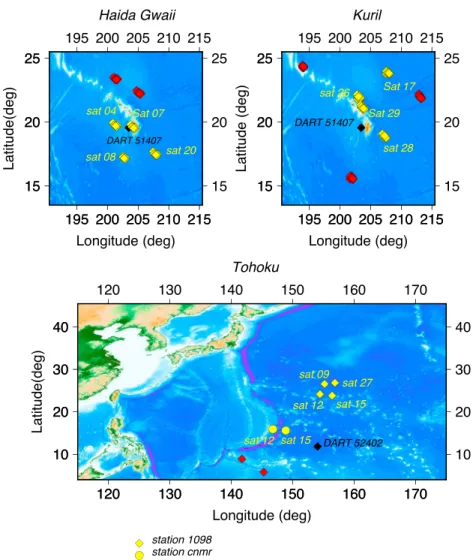
We inverted all the TEC data related to these four satellites. The location of the IPP at 300 km at the time of the maximum perturbation used for all the inverted satellite-station pairs (yellow squares) and the location of the reconstructed DART buoy (black squares) are shown in Figure 6 for the three events.
Figure 6. Location of the IPP at 300 km at the time of the maximum perturbation of each inverted station-satellite pair
is shown in yellow. The red diamonds correspond to the satellites for which the signal-to-noise ratio was too small to perform an inversion. The black square corresponds to the location of the DART buoy where the tsunami was reconstructed.
The Haida Gwaii and Kuril inversions were colocated (the TEC measurement and tsunami height reconstruc-tion are at almost the exact same locareconstruc-tion), but this was not the case for Tohoku, which was about 1,400 km (station 1098) and 970 km (station cnmr) from the other two close locations.
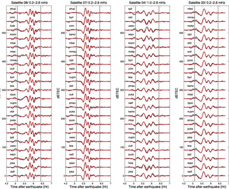
The results of TEC inversion for the station-satellite pairs are shown in Figures 7–9 for the 2012 Haida Gwaii, 2006 Kuril, and the 2011 Tohoku events, respectively. The tsunami wave height reconstructed from these inversions at reference DART locations is shown in Figure 10.
We were able to obtain a fairly accurate estimate of the peak-to-peak tsunami height amplitude through these TEC inversions, with a fit comparable to the DART data for the three events and for almost all the satellite-station pairs. The inversion of the Tohuku event TEC signature furthermore shows that this inversion can predict the maximum amplitude of the tsunami height, even when the TEC measurements and tsunami reconstruction are not colocated.
4.4. Limits and Future Improvement Directions: The Case of Tohoku in Hawaii
TEC observations in Hawaii of the Tohoku tsunami were the most challenging due to both a larger noise and a smaller than modeled signal: geomagnetic conditions were indeed bad with a large Dst, and in addi-tion, observations in Hawaii were made at about 2 h 45 Local time with southeastward propagation path, which corresponds to condition in which both the lower background TEC and a likely eastward zonal wind (Drob et al., 2015) might reduce significantly TEC-tsunami induced perturbation (e.g., Hickey et al., 2009).
Figure 7. Haida Gwaii TEC inversion. The data are in black and the inverted time series in red. The vertical gray lines correspond to the inversion time window.
From left to right, results for satellites 08, 07, 04, and 20 observed by 25 GPS stations. Band-pass filtering is applied from 0.2 mHz to 2.6 mHz.
Note, in contrary, that Haida Gwaii corresponds to a southward path, in which zonal wind are almost orthog-onal and with smaller impact (Hickey et al., 2009), while Kurils was observed in the morning in Hawaii Local time (8 h 45) and at a time where the zonal wind was likely westward (Drob et al., 2015). These conditions explain likely why our first attempt to inverse the Tohoku data in Hawaii, with the same 0.2 mHz and 2.6 mHz bandwidth as used for the two other tsunami, failed. This is clearly understood with Figure 11, which shows the comparison between the power spectrum density of the GPS data and the inverted TEC both in the case of Haida Gwaii and Tohoku and for GPS stations ahup and yeep, respectively. In the Tohoku’s spectrum, large amplitudes in the GPS data spectrum below 0.5 mHz are observed, not found for the geomagnetic quiet Haida Gwaii TEC spectrum and likely due to the geomagnetic storm which occurred on the day of the Tohoku earthquake. Figure 12 shows, however, the results of the TEC inversion with a filter between 0.5 mHz and 2.6 mHz, which better reject the large low-frequency noise. A reasonable estimation of the tsunami height is then obtained, when compared to the DART data. Although more positive, this example shows nevertheless that future improvements will have not only to better remove the TEC background but will likely have to also introduce winds in the modeling and possibly waveform inversion.
Figure 8. Kuril TEC inversion. The data are in black and the inverted time series in red. The vertical gray lines correspond to the inversion time window. Band-pass
filtering is applied from 1.0 mHz to 2.6 mHz.
5. Statistics of the Inversion
Estimating the statistics of success for this new tsunami height inversion strategy is mandatory if it is to be of use for tsunami warning systems. Even though more analysis will be required to consolidate these statistics, the three examples described above provide a primary data set. In order to study the statistics of this
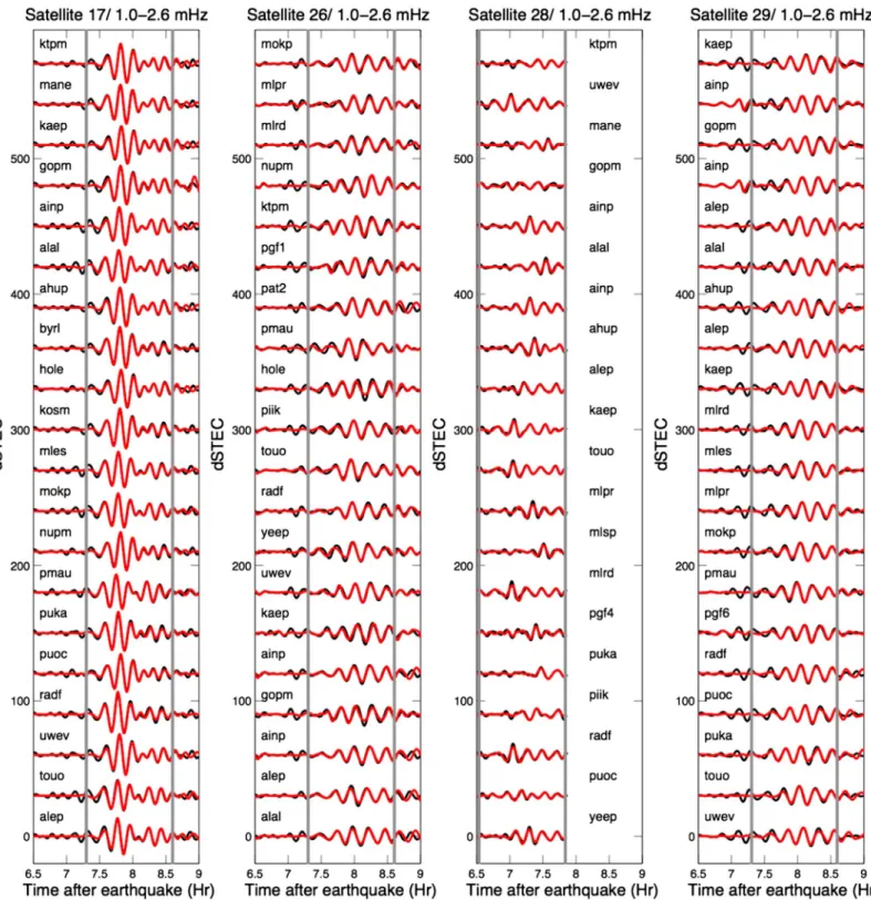
Figure 9. Tohoku tsunami TEC inversion. The data are in black and the inverted time series in red. The vertical gray lines
correspond to the inversion time window. Band-pass filtering is applied from 0.2 to 2.6 mHz.
Figure 10. Tsunami height reconstruction from the TEC inversion of Haida Gwaii (top), Kuril (middle), and Tohoku
(bottom) tsunami events. The DART data are in black, the reconstructed time series in gray, and their averaged time series in red.
Figure 11. Power density spectrum of the TEC-GPS data (black) and the TEC inversion (red) for the Haida Gwaii case
(left) and the Tohoku case (right).
Figure 12. TEC inversion of the satellite 25-yeep station pair (top) and tsunami reconstruction from DART buoy 51407
Figure 13. Statistical study of peak-to-peak tsunami height for Haida Gwaii, Kuril, and Tohoku tsunami events. The red
curve corresponds to a Gaussian fit of each distribution.
inversion technique, we must first define the amplitude error inversion𝜖 as follows:
𝜖 = hTEC
hDART, (19)
where hTECis the maximum peak to peak amplitude obtained by the TEC reconstruction and hDARTis that measured by the DART buoy. The closer𝜖 is to 1 the better our inversion. Figure 13 shows the histogram of the distribution of𝜖 for Haida Gwaii, Kuril, and Tohoku. The red curve corresponds to an ideal Gaussian distribution and reveals a tendency for our method to underestimate the tsunami height. The estimation of the tsunami amplitude for Haida Gwaii is fairly good. Indeed, we were able to predict the 2 cm peak-to-peak tsunami amplitude with an error of less than 10% for 95% of the inverted satellite-station pairs. For Kuril, we managed to estimate the 3 cm peak-to-peak amplitude of the tsunami with an error of less than 20% for 80% of the time series inverted. For Tohoku, we estimated the 55 cm peak-to-peak amplitude of the tsunami with an error of less than 10% for 95% of the time series inverted.
Thus, the inversion method applied to Haida Gwaii and Tohoku works far better for them than for the Kuril case. This can also be seen in the mean value of𝜖 which is closer to 1, with a smaller standard deviation in the Haida Gwaii case. This could be explained by the fact that the source in the Kuril Islands tsunami case is more complex.
6. Resolution of the Inversion
In order to estimate the resolution of the inversion and its sensitivity to ionospheric background noise, we inverted the same satellite-station pairs for the three events 1 day and 1 year before the earthquake and tsunami. The histogram of the reconstructed peak-to-peak amplitude is shown in Figure 14. The inversion for Haida Gwaii and Kuril 1 day before the event and 1 year before the event both led to a very small reconstructed tsunami (about 0.5 cm peak to peak). The noise𝜎 has been calculated with the TEC data measured 1 day before for Haida Gwaii and Kuril and both the data measured 1 day before and 1 year before for Tohoku. This reconstructed a false positive tsunami with a 2.5 mm amplitude corresponds to good ionospheric conditions
Figure 14. Statistical study of peak-to-peak tsunami height for Haida Gwaii, Kuril, and Tohoku events when the inversion
method is applied to the data on the day of the event (left), 1 day before (center), and 1 year before (right) for each tsunami event. Note the change of scale of the Tohoku tsunami wave height estimation (bottom left).
(quiet ionosphere). In the case of Tohoku, the inversion 1 year before the event also generates a very small reconstructed tsunami (about 0.5 cm peak to peak). However, 1 day before the event, the inversion generates a tsunami with a peak-to-peak amplitude of 2–3 cm. The high amplitude obtained may be explained by the fact that a geomagnetic storm occurred that day. Dst was about −62 nT, whereas it was about −35 nT 1 day before, −16 nT 1 year before, 0 nT the day of Haida Gwaii tsunami, and −13 nT in the day of Kuril tsunami. Thus, the resolution of the inversion strongly depends on ionospheric conditions. This is one of the limitations of our method. It can be improved by jointly inverting several TEC sounding points (one receiver and all the satellites within range), which provides a way of selecting only the Travelling Ionospheric Disturbances (TIDs) propagating with the expected azimuth associated with the quake being sought and taking into account measurement noise. However, this is far beyond the scope of this study, which aims to demonstrate the fea-sibility of using TEC data alone to constrain the tsunami height at ocean level and very likely improve the performance of TEC tsunami inversions.
7. Conclusion
In this paper, we have presented an least squares inversion strategy for tsunami height based on the inversion of single TEC records. This has been tested for three tsunami events. The technique is based on a tsunami normal-mode summation method that explicitly integrates the coupling of modes with the atmosphere and ionosphere. The excitation coefficients of normal modes are first estimated from the TEC data and then used to reconstruct the tsunami waveform. These excitation coefficients are found by seeking the best local moment tensor from TEC waveform fitting. After numerical validation with simulated data, we have shown that an inversion with two local moment tensor sources is, as expected, more realistic than an inversion with one source and allows reconstruction of the first tsunami wave packet and therefore the main peak of the tsunami height measured by the DART buoy. Some limitations remain in the waveform inversion, such as the signature in both the TEC and tsunami waveforms of the arrival of the second group of waves most likely due to coastal reflection. This could be enhanced in the future either by modeling the tsunami waveform near the coast better, or by adding additional sources.
Using the huge potential of the widespread GPS station network in Hawaii, we showed that the proposed TEC inversion provides a fairly good estimation of the tsunami height for 75% of the satellite-station pairs available at the time of the arrival of the 2012 Haida Gwaii tsunami and of the 2006 Kuril Islands tsunami in Hawaii. This result was confirmed by the successful inversion of two stations located in the Northwest Pacific in the case of the 2011 Tohoku tsunami (closer field). The key limitation in these three examples is the sounding geom-etry of the TEC path and its configuration with respect to the magnetic field, which is optimal for only 75% of the satellites within station range. This limitation will be reduced in the future when other GNSS systems
such as Galileo, GLONASS, or BeiDou become fully available. When there is little ionospheric activity and for a tsunami with a 2–3 cm peak-to-peak range, the tsunami height is successfully forecast in over 80% of cases with an error of less than 20%. The tsunami wave height can furthermore be estimated even when the TEC inversion is performed a long way from the area where the tsunami height has to be estimated, as demon-strated with the last inversion performed for the Tohuku tsunami. When there is substantial ionospheric activity, the error is likely to increase and it appears necessary to invert several TEC signals in order to obtain comparable measurement errors. Our results nevertheless demonstrate that inverting the TEC to retrieve a tsunami waveform may be a very efficient way of completing the tsunami warning system with data cover-ing areas where no DART systems have been deployed or when the DART systems are temporarily down. The inversion process is moreover very quick to perform, especially if tsunami normal modes are precomputed for a range of possible locations, local time, and solar flux (F10.7) index, offering the possibility of near-real-time computations in the future.
Appendix A
Let us note P as the transfer matrix between the spherical basis and the eigenvector basis. In this chapter, all the quantities expressed in the eigenvector basis are noted with an E superscript. As matrix A is invertible, equation (16) can thus be rewritten:
P−1APP−1m = PP−1b. (A1)
This can be simplified into
AEmE= bE (A2)
It should be remembered that
⎧ ⎪ ⎪ ⎨ ⎪ ⎪ ⎩ AE = P−1AP mE = P−1m bE = P−1b (A3)
In index notation the system is written as
AEijmEj = bEi, (A4)
From the definition of the matrix AEwe can deduce
mEi = b E i
𝜆i
, (A5)
where𝜆iare the eigenvalues of A. As the three smallest values of𝜆iare not related to vertical motion and do not excite the tsunami, the associated value mE
i will not be taken into account in the inversion and be set to 0. Thus, the moment tensor in spherical basis finally reads
mi=∑ j
PijmE
j (A6)
References
Artru, J., Ducic, V., Kanamori, H., Lognonné, P., & Murakami, M. (2005). Ionospheric detection of gravity waves induced by tsunamis.
Geophysical Journal International, 160(3), 840–848. https://doi.org/10.1111/j.1365-246X.2005.02552.x
Artru, J., Farges, T., & Lognonné, P. (2004). Acoustic waves generated from seismic surface waves: Propagation properties determined from Doppler sounding observations and normal-mode modelling. Geophysical Journal International, 158(3), 1067–1077. https://doi.org/10.1111/j.1365-246X.2004.02377.x
Artru, J., Lognonné, P., & Blanc, E. (2001). Normal modes modelling of post-seismic ionospheric oscillations. Geophysical Research Letters,
28(4), 697–700. https://doi.org/10.1029/2000GL000085
Bilitza, D., & Reinisch, B. W. (2008). International reference ionosphere 2007: Improvements and new parameters. Advances in Space
Research, 42(4), 599–609. https://doi.org/10.1016/j.asr.2007.07.048
Chum, J., Cabrera, M., Mošna, Z., Fagre, M., Baše, J., & Fišer, J. (2016). Nonlinear acoustic waves in the viscous thermosphere and ionosphere above earthquake. Journal of Geophysical Research: Space Physics, 121, 12,126–12,137. https://doi.org/10.1002/2016JA023450 Coïsson, P., Lognonné, P., Walwer, D., & Rolland, L. M. (2015). First tsunami gravity wave detection in ionospheric radio occultation data.
Earth and Space Science, 2, 125–133. https://doi.org/10.1002/2014EA000054
Acknowledgments
This work has been fully supported by the U.S. Office of Naval Research through the TWIST project (ONR grant N000141310035 and ONR Global grant N62909-13-1-N270), and we acknowledge the additional support offered to V. R. by ED STEP’UP and IUF for P. L. We would also like to thank M. Drilleau, E. Astafyeva, G. Occhipinti, Y. Nishikawa, F. Karakostas, and A. Sladen for fruitful discussions. We are grateful to the operators of the SOPAC, GEONET, and DART networks for providing the data used in this study.
Drob, D. P., Emmert, J. T., Meriwether, J. W., Makela, J. J., Doornbos, E., Conde, M., et al. (2015). An update to the horizontal wind model (HWM): The quiet time thermosphere. Earth and Space Science, 2, 301–319. https://doi.org/10.1002/2014ea000089
Dziewonski, A., Chou, T.-A., & Woodhouse, J. (1981). Determination of earthquake source parameters from waveform data for studies of global and regional seismicity. Journal of Geophysical Research, 86(B4), 2825–2852. https://doi.org/10.1029/JB086iB04p02825 Dziewonski, A. M., & Anderson, D. L. (1981). Preliminary reference Earth model. Physics of the Earth and Planetary Interiors, 25(4), 297–356.
https://doi.org/10.1016/0031-9201(81)90046-7
Fan, G., & Wallace, T. (1991). The determination of source parameters for small earthquakes from a single, very broadband seismic station.
Geophysical Research Letters, 18(8), 1385–1388. https://doi.org/10.1029/91GL01804
Galvan, D. A., Komjathy, A., Hickey, M. P., & Mannucci, A. J. (2011). The 2009 Samoa and 2010 Chile tsunamis as observed in the ionosphere using GPS total electron content. Journal of Geophysical Research, 116, A06318. https://doi.org/10.1029/2010JA016204
Godin, O. A., Zabotin, N. A., & Bullett, T. W. (2015). Acoustic-gravity waves in the atmosphere generated by infragravity waves in the ocean.
Earth, Planets and Space, 67(1), 47. https://doi.org/10.1186/s40623-015-0212-4
Grawe, M. A., & Makela, J. J. (2015). The ionospheric responses to the 2011 Tohoku, 2012 Haida Gwaii, and 2010 Chile tsunamis: Effects of tsunami orientation and observation geometry. Earth and Space Science, 2, 472–483. https://doi.org/10.1002/2015EA000132.1 Grawe, M. A., & Makela, J. J. (2017). Observation of tsunami-generated ionospheric signatures over Hawaii caused by the 16 September
2015 Illapel earthquake. Journal of Geophysical Research: Space Physics, 122, 1128–1136. https://doi.org/10.1002/2016JA023228 Hayes, G. P. (2011). Rapid source characterization of the 2011Mw9.0 off the Pacific Coast of Tohoku earthquake. Earth, Planets and Space,
63(7), 4. https://doi.org/10.5047/eps.2011.05.012
Hickey, M. P., Schubert, G., & Walterscheid, R. L. (2009). Propagation of tsunami-driven gravity waves into the thermosphere and ionosphere.
Journal of Geophysical Research, 114, A08304. https://doi.org/10.1029/2009JA014105
Hines, C. (1972). Gravity waves in the atmosphere. Nature, 239(5367), 73–78. https://doi.org/10.1038/239073a0
Hooke, W. H. (1970). The ionospheric response to internal gravity waves: 1. The F2 region response. Journal of Geophysical Research, 75(28), 5535–5544. https://doi.org/10.1029/JA075i028p05535
Kamogawa, M., Orihara, Y., Tsurudome, C., Tomida, Y., Kanaya, T., Ikeda, D., et al. (2016). A possible space-based tsunami early warning system using observations of the tsunami ionospheric hole. Scientific Reports, 6(37), 989. https://doi.org/10.1038/srep37989 Kherani, E. A., Lognonné, P., Hébert, H., Rolland, L., Astafyeva, E., Occhipinti, G., et al. (2012). Modelling of the total electronic content
and magnetic field anomalies generated by the 2011 Tohoku-Oki tsunami and associated acoustic-gravity waves. Geophysical Journal
International, 191(3), 1049–1066. https://doi.org/10.1111/j.1365-246X.2012.05617.x
Kherani, E. A., Rolland, L., Lognonné, P., Sladen, A., Klausner, V., & de Paula, E. R. (2016). Traveling ionospheric disturbances propagating ahead of the Tohoku-Oki tsunami: A case study. Geophysical Journal International, 204(2), 1148–1158. https://doi.org/10.1093/gji/ggv500 Kim, S., Kraeva, N., & Chen, Y.-T. (2000). Source parameter determination of regional earthquakes in the far east using moment tensor
inversion of single-station data. Tectonophysics, 317(1), 125–136. https://doi.org/10.1016/S0040-1951(99)00274-7
Liu, J.-Y., Tsai, Y.-B., Ma, K.-F., Chen, Y.-I., Tsai, H.-F., Lin, C.-H., et al. (2006). Ionospheric GPS total electron content (TEC) disturbances triggered by the 26 December 2004 Indian Ocean tsunami. Journal of Geophysical Research, 111, A05303. https://doi.org/10.1029/2005JA011200 Lognonné, P. (1991). Normal modes and seismograms in an anelastic rotating Earth. Journal of Geophysical Research, 96(B12),
20,309–20,319. https://doi.org/10.1029/91JB00420
Lognonné, P., Artru, J., Garcia, R., Crespon, F., Ducic, V., Jeansou, E., et al. (2006). Ground-based GPS imaging of ionospheric post-seismic signal. Planetary and Space Science, 54(5), 528–540. https://doi.org/10.1016/j.pss.2005.10.021
Lognonné, P., Clévédé, E., & Kanamori, H. (1998). Computation of seismograms and atmospheric oscillations by normal-mode summation for a spherical Earth model with realistic atmosphere. Geophysical Journal International, 135(2), 388–406. https://doi.org/10.1046/j.1365-246X.1998.00665.x
Lognonné, P., Karakostas, F., Rolland, L., & Nishikawa, Y. (2016). Modeling of atmospheric-coupled Rayleigh waves on planets with atmosphere: From Earth observation to Mars and Venus perspectives. The Journal of the Acoustical Society of America, 140(2), 1447–1468. https://doi.org/0001-4966/2016/140(2)/1447/22
MacDoran, P. F. (1981). Series satellite emission radio interferometric Earth surveying. In Third Annual NASA Geodynamics Program Review,
Crustal Dynamics Project, Geodynamics Research (pp. 76). Washington, DC: NASA.
Macleod, M. A. (1966). Sporadic E theory. I. Collision-geomagnetic equilibrium. Journal of the Atmospheric Sciences, 23(1), 96–109. Mai, C.-L., & Kiang, J.-F. (2009). Modeling of ionospheric perturbation by 2004 Sumatra tsunami. Radio Science, 44, RS3011.
https://doi.org/10.1029/2008RS004060
Mannucci, A., Wilson, B., Yuan, D., Ho, C., Lindqwister, U., & Runge, T. (1998). A global mapping technique for GPS-derived ionospheric total electron content measurements. Radio Science, 33, 565–582. https://doi.org/10.1029/97RS02707
Maus, S., MacMillan, S., Chernova, T., Choi, S., Dater, D., Golovkov, V., et al. (2005). The 10th-generation international geomagnetic reference field. Geophysical Journal International, 161(3), 561–565. https://doi.org/10.1016/j.pepi.2005.03.006
Meng, X., Komjathy, A., Verkhoglyadova, O. P., Yang, Y. M., Deng, Y., & Mannucci, A. J. (2015). A new physics-based modeling approach for tsunami-ionosphere coupling. Geophysical Research Letters, 42, 4736–4744. https://doi.org/10.1002/2015GL064610
National Research Council (2011). Tsunami warning and preparedness: an assessment of the US tsunami program and the nation’s pre-paredness efforts, Committee on the Review of the Tsunami Warning and Forecast System and Overview of the Nation’s Tsunami Preparedness, National Research Council (284 pp.).
Occhipinti, G., Coïsson, P., Makela, J. J., Allgeyer, S., Kherani, A., Hébert, H., & Lognonné, P. (2011). Three-dimensional numerical modeling of tsunami-related internal gravity waves in the Hawaiian atmosphere. Earth, Planets and Space, 63(7), 847–851. https://doi.org/10.5047/eps.2011.06.051
Occhipinti, G., Kherani, A. E., & Lognonné, P. (2008). Geomagnetic dependence of ionospheric disturbances induced by tsunamigenic internal gravity waves. Geophysical Journal International, 173(3), 753–765. https://doi.org/10.1111/j.1365-246X.2008.03760.x
Occhipinti, G., Lognonné, P., Kherani, E. A., & Hébert H. (2006). Three-dimensional waveform modeling of ionospheric signature induced by the 2004 Sumatra tsunami. Geophysical Research Letters, 33, L20104. https://doi.org/10.1029/2006GL026865
Okal, E. A. (1982). Mode-wave equivalence and other asymptotic problems in tsunami theory. Physics of the Earth and Planetary Interiors,
30(1), 1–11. https://doi.org/10.1016/0031-9201(82)90123-6
Peltier, W. R., & Hines, C. O. (1976). On the possible detection of tsunamis by a monitoring of the ionosphere. Journal of Geophysical Research,
81(12), 1995–2000. https://doi.org/10.1029/JC081i012p01995
Phinney, R. A., & Burridge, R. (1973). Representation of the elastic-gravitational excitation of a spherical Earth model by generalized spherical harmonics. Geophysical Journal International, 34(4), 451–487. https://doi.org/10.1111/j.1365-246X.1973.tb02407.x Picone, J. M., Hedin, A. E., Drob, D. P., & Aikin, A. C. (2002). NRLMSISE-00 empirical model of the atmosphere: Statistical comparisons and
Rakoto, V., Lognonné, P., & Rolland, L. (2017). Tsunami modeling with solid earth-ocean-atmosphere coupled normal modes. Geophysical
Journal International, 211(2), 1119–1138.
Rolland, L. M., Lognonné, P., Astafyeva, E., Kherani, E. A., Kobayashi, N., Mann, M., & Munekane, H. (2011). The resonant response of the ionosphere imaged after the 2011 off the Pacific Coast of Tohoku earthquake. Earth, Planets and Space, 63(7), 853–857. https://doi.org/10.5047/eps.2011.06.020
Rolland, L. M., Lognonné, P., & Munekane, H. (2011). Detection and modeling of Rayleigh wave induced patterns in the ionosphere.
Journal of Geophysical Research, 116, A05320. https://doi.org/10.1029/2010JA016060
Rolland, L. M., Occhipinti, G., Lognonné, P., & Loevenbruck, A. (2010). Ionospheric gravity waves detected offshore Hawaii after tsunamis.
Geophysical Research Letters, 37, L17101. https://doi.org/10.1029/2010GL044479
Satake, K. (2002). Tsunamis. In W. H. K. Lee, et al. (Eds.), International Handbook of Earthquake and Engineering Seismology, Part A, Int.
Geophys. Ser. (Vol. 81A, pp. 437–451). San Francisco, CA: Academic Press.
Savastano, G., Komjathy, A., Verkhoglyadova, O., Mazzoni, A., Crespi, M., Wei, Y., & Mannucci, A. J. (2017). Real-time detection of tsunami ionospheric disturbances with a stand-alone GNSS receiver: A preliminary feasibility demonstration. Scientific Reports, 7, 46607. Stein, S., & Okal, E. A. (2007). Ultralong period seismic study of the December 2004 Indian Ocean earthquake and implications for regional
tectonics and the subduction process. Bulletin of the Seismological Society of America, 97(1A), S279–S295.
Titov, V., Rabinovich, A. B., Mofjeld, H. O., Thomson, R. E., & González, F. I. (2005). The global reach of the 26 December 2004 Sumatra tsunami.
Science, 309, 2045–2048. https://doi.org/10.1126/science.1114576
Vadas, S. L., Makela, J. J., Nicolls, M. J., & Milliff, R. F. (2015). Excitation of gravity waves by ocean surface wave packets: Upward propagation and reconstruction of the thermospheric gravity wave field. Journal of Geophysical Research: Space Physics, 120, 1–33.
https://doi.org/10.1002/2015JA021430
Walter, W. R. (1993). Source parameters of the June 29, 1992 Little Skull Mountain earthquake from complete regional waveforms at a single station. Geophysical Research Letters, 20(5), 403–406. https://doi.org/10.1029/92GL03031
Ward, S. N. (1980). Relationships of tsunami generation and an earthquake source. Journal of Physics of the Earth, 28(5), 441–474. https://doi.org/10.4294/jpe1952.28.441
Watada, S., Kusumoto, S., & Satake, K. (2014). Traveltime delay and initial phase reversal of distant tsunamis coupled with the self-gravitating elastic Earth. Journal of Geophysical Research: Solid Earth, 119, 4287–4310. https://doi.org/10.1002/2013JB010841
Zhang, X., & Tang, L. (2015). Detection of ionospheric disturbances driven by the 2014 Chile tsunami using GPS total electron content in New Zealand. Journal of Geophysical Research: Space Physics, 120, 7918–7925. https://doi.org/10.1002/2014JA020879