HAL Id: hal-02976236
https://hal.archives-ouvertes.fr/hal-02976236
Submitted on 26 Oct 2020
HAL is a multi-disciplinary open access
archive for the deposit and dissemination of
sci-entific research documents, whether they are
pub-lished or not. The documents may come from
teaching and research institutions in France or
abroad, or from public or private research centers.
L’archive ouverte pluridisciplinaire HAL, est
destinée au dépôt et à la diffusion de documents
scientifiques de niveau recherche, publiés ou non,
émanant des établissements d’enseignement et de
recherche français ou étrangers, des laboratoires
publics ou privés.
Antarctica in 1960–2013: observations and simulations
from the ECHAM5-wiso atmospheric general circulation
model
Sentia Goursaud, Valérie Masson-Delmotte, Vincent Favier, Anaïs Orsi,
Martin Werner
To cite this version:
Sentia Goursaud, Valérie Masson-Delmotte, Vincent Favier, Anaïs Orsi, Martin Werner. Water stable
isotope spatio-temporal variability in Antarctica in 1960–2013: observations and simulations from the
ECHAM5-wiso atmospheric general circulation model. Climate of the Past, European Geosciences
Union (EGU), 2018, 14 (6), pp.923-946. �10.5194/cp-14-923-2018�. �hal-02976236�
https://doi.org/10.5194/cp-14-923-2018
© Author(s) 2018. This work is distributed under the Creative Commons Attribution 4.0 License.
Water stable isotope spatio-temporal variability in Antarctica
in 1960–2013: observations and simulations from the
ECHAM5-wiso atmospheric general circulation model
Sentia Goursaud1,2, Valérie Masson-Delmotte1, Vincent Favier1, Anaïs Orsi2, and Martin Werner3 1Univ. Grenoble Alpes, CNRS, IGE, F-38000 Grenoble, France
2LSCE (Institut Pierre Simon Laplace, UMR CEA-CNRS-UVSQ 8212, Université Paris Saclay), Gif-sur-Yvette, France 3Alfred Wegener Institute, Helmholtz Centre for Polar and Marine Research, Bremerhaven, Germany
Correspondence:Sentia Goursaud (sentia.goursaud@lsce.ipsl.fr) Received: 25 September 2017 – Discussion started: 18 December 2017 Revised: 4 May 2018 – Accepted: 8 June 2018 – Published: 28 June 2018
Abstract. Polar ice core water isotope records are com-monly used to infer past changes in Antarctic temperature, motivating an improved understanding and quantification of the temporal relationship between δ18O and temperature. This can be achieved using simulations performed by at-mospheric general circulation models equipped with water stable isotopes. Here, we evaluate the skills of the high-resolution water-isotope-enabled atmospheric general circu-lation model ECHAM5-wiso (the European Centre Ham-burg Model) nudged to European Centre for Medium-Range Weather Forecasts (ECMWF) reanalysis using simulations covering the period 1960–2013 over the Antarctic continent. We compare model outputs with field data, first with a fo-cus on regional climate variables and second on water stable isotopes, using our updated dataset of water stable isotope measurements from precipitation, snow, and firn–ice core samples. ECHAM5-wiso simulates a large increase in tem-perature from 1978 to 1979, possibly caused by a disconti-nuity in the European Reanalyses (ERA) linked to the assim-ilation of remote sensing data starting in 1979.
Although some model–data mismatches are observed, the (precipitation minus evaporation) outputs are found to be realistic products for surface mass balance. A warm model bias over central East Antarctica and a cold model bias over coastal regions explain first-order δ18O model biases by too-strong isotopic depletion on coastal areas and underestimated depletion inland. At the second order, despite these biases, ECHAM5-wiso correctly captures the observed spatial pat-terns of deuterium excess. The results of model–data com-parisons for the inter-annual δ18O standard deviation
dif-fer when using precipitation or ice core data. Further stud-ies should explore the importance of deposition and post-deposition processes affecting ice core signals and not re-solved in the model.
These results build trust in the use of ECHAM5-wiso outputs to investigate the spatial, seasonal, and inter-annual δ18O–temperature relationships. We thus make the first Antarctica-wide synthesis of prior results. First, we show that local spatial or seasonal slopes are not a correct surrogate for inter-annual temporal slopes, leading to the conclusion that the same isotope–temperature slope cannot be applied for the climatic interpretation of Antarctic ice core for all timescales. Finally, we explore the phasing between the seasonal cycles of deuterium excess and δ18O as a source of information on changes in moisture sources affecting the δ18O–temperature relationship. The few available records and ECHAM5-wiso show different phase relationships in coastal, intermediate, and central regions.
This work evaluates the use of the ECHAM5-wiso model as a tool for the investigation of water stable isotopes in Antarctic precipitation and calls for extended studies to im-prove our understanding of such proxies.
1 Introduction
The Antarctic climate has been monitored from sparse weather stations providing instrumental records starting at best in 1957 (Nicolas and Bromwich, 2014). Water stable isotopes in Antarctic ice cores are key to expanding the
documentation of spatio-temporal changes in polar climate and the hydrologic cycle (Jouzel et al., 1997) for the recent past (PAGES 2k Consortium, 2013; Stenni et al., 2017) as well as for glacial–interglacial variations (Jouzel et al., 2007; Schoenemann et al., 2014). Water stable isotopes measured along ice cores were initially used to infer Antarctic past tem-peratures using the spatial isotope–temperature slope (Lorius et al., 1969). The focus on inter-annual variations is moti-vated by the goal of quantifying temperature changes at the Earth’s surface, including Antarctica, during the last millen-nia, to place current changes in the perspective of recent nat-ural climate variability (Jones et al., 2016), to understand the drivers of this variability, and to test the ability of climate models to correctly represent it. This timescale is relevant for the response of the Antarctic climate to e.g. volcanic forcing and for the Antarctic climate fingerprint of large-scale modes of variability such as ENSO and the Southern Annular Mode (Smith and Stearns, 1993; Turner, 2004; Stammerjohn et al., 2008; Schroeter et al., 2017). The various climate signals po-tentially recorded in precipitation isotopic composition are, however, difficult to disentangle.
First, the original signal from precipitation may be altered due to deposition and post-deposition processes (e.g. Sokra-tov and Golubev, 2009; Jones et al., 2017; Münch et al., 2017; Laepple et al., 2018). Wind erosion and sublimation during or after precipitation have long been known to affect ice core records (Eisen et al., 2008; Grazioli et al., 2017). Other pro-cesses such as melt and diffusion can also alter the preser-vation of isotopic signals in firn and ice and cause smooth-ing of the initial snowfall signals (Johnsen, 1977; Whillans and Grootes, 1985; Johnsen et al., 2000; Jones et al., 2017). So far, the mechanisms of such post-deposition processes on the alteration of the initial precipitation signals are not fully understood and quantified (Touzeau et al., 2017). Sec-ond, the Antarctic snowfall isotopic composition may be af-fected by the origin of moisture and the associated evapo-ration conditions, changes in the relationship between con-densation and surface temperature, or changes in the inter-mittency of precipitation (e.g. Sime et al., 2009; Hoshina et al., 2014; Touzeau et al., 2016). Although the surface snow isotopic composition signal has classically been interpreted as a precipitation-weighted deposition signal (Krinner and Werner, 2003), recent studies evidenced isotopic exchanges between the Antarctic snow surface and the atmosphere as-sociated with snow metamorphism occurring at diurnal and sub-annual scales (Steen-Larsen et al., 2014; Casado et al., 2016; Ritter et al., 2016; Touzeau et al., 2016).
Second, the climatic interpretation of water stable isotopes in Antarctic ice cores is still challenging. Quantitative ap-proaches have relied on empirical relationships and the use of theoretical and atmospheric models including water stable isotopes. Pioneer studies evidenced a close linear relation-ship between the spatial distribution of water stable isotopes and local temperature (e.g. Lorius and Merlivat, 1975) and explained this feature as the result of the distillation along
air mass trajectories. Thereupon, local temperature (i.e. at a specific site) was reconstructed using δ18O measurements and based on the slope of the aforementioned spatial em-pirical relationship as a surrogate for relationships at annual to multi-annual scales. However, recent data syntheses have shown that other effects had to be taken into account (e.g. Masson-Delmotte et al., 2008). It was found that Antarc-tic snowfall isotopic composition is also linked to the ini-tial vapour isotopic composition (Stenni et al., 2016), atmo-spheric transport pathways (Schlosser et al., 2008; Dittmann et al., 2016), Antarctic sea ice extent (Bromwich and Weaver, 1983; Noone and Simmonds, 2004; Holloway et al., 2016), and local condensation temperature, which is itself related to surface temperature through complex boundary layer pro-cesses (Krinner et al., 2007). Evaporation conditions, trans-port, and boundary layer processes may vary through time from seasonal (Fernandoy et al., 2018) to annual or multi-annual scale, thereby potentially distorting the quantitative relationship between snow isotopic composition and local surface air temperature estimated empirically for present-day conditions (Jouzel et al., 1997).
Model studies have been key to quantitatively exploring the spatio-temporal aspects of the relationships between pre-cipitation isotopic composition and temperature (Jouzel et al., 2000). Mixed-cloud isotopic models have been used to propose a coherent interpretation of δ18O and δD data in terms of changes in site and source temperatures (Uemura et al., 2012) or to simulate isotopic variations along individ-ual atmospheric trajectories (Dittmann et al., 2016). How-ever, such theoretical distillation models rely on the clo-sure assumption at the ocean surface to calculate the initial evaporation isotopic composition and do not account for at-mospheric dynamics and mixing of air masses (Jouzel and Koster, 1996; Delmotte et al., 2000). Atmospheric general circulation models equipped with water stable isotopes of-fer a physically coherent, three-dimensional framework to investigate the weather and climate drivers of Antarctic pre-cipitation isotopic composition (Jouzel et al., 2000). They play a key role in assessing how different boundary condi-tions (e.g. changes in orbital forcing, changes in atmospheric greenhouse gas concentration) affect the simulated relation-ships between precipitation isotopic composition and climate variables. Most of these simulations support the idea that the present-day isotope–temperature spatial relationship is a good approximation for the relationships between glacial conditions and today (Delaygue et al., 2000; Werner et al., 2018), with one exception (Lee et al., 2008). One study used climate projections in response to increased atmospheric CO2 concentration to explore isotope–temperature relation-ships in a world warmer than today and suggested a ing temporal isotope–temperature relationship due to chang-ing covariance between temperature and precipitation (Sime et al., 2009). Several observational and modelling studies have also evidenced different isotope–temperature relation-ships between the spatial relationship and those calculated at
Figure 1.Spatial distribution of Antarctica in seven regions: East Antarctic Plateau, coastal Indian, Weddell sea, West Antarctic Ice Sheet, Victoria Land, and Dronning Maud Land. The location of the selected READER surface stations: Neumayer, Mawson, Vostok, Dome C, Casey, Dumont d’Urville (noted as “DDU”), McMurdo, Byrd, Palmer, and Esperanza.
the seasonal (Morgan and van Ommen, 1997) or inter-annual scale (Schmidt et al., 2007).
Our study is motivated by the need for a synthesis over all of Antarctica using a proper interpretation of processes that affect water stable isotopes on the appropriate spatial and temporal scales. It aims to address the following questions: (i) what is the performance of a state-of-the-art atmospheric general circulation model with respect to existing Antarc-tic observations of spatio-temporal variations in temperature, surface mass balance, precipitation, and snow isotopic com-position for present day? (ii) What can we learn from such a model for the regional relationships between isotopic com-position from the precipitation and temperature at the inter-annual scale for the recent past and considering all of Antarc-tica?
For this purpose, we focus on the high-resolution atmo-spheric general circulation model equipped with water sta-ble isotopes, ECHAM5-wiso (the European Centre Hamburg model), which demonstrated remarkable skills for Antarctica (Werner et al., 2011). We explore a simulation performed for the period 1960–2013 in which the atmospheric model is nudged to the European Reanalyses (ERA) ERA-40 and ERA-Interim (Uppala et al., 2005), ensuring that the day-to-day simulated variations are coherent with the observed day-to-day variations in synoptic weather and atmospheric circulation (see Butzin et al., 2014, for more explanation). This framework is crucial to performing comparisons be-tween simulations and observations for temporal variations. Second, we compile a database of precipitation, snow, and
firn–ice isotopic composition using data from precipitation sampling and ice core records and considering δ18O and deu-terium excess (hereafter, d). These methods are described in Sect. 2. We then compare the model outputs with the available datasets (Sect. 3). After evaluating the near-surface temperature and the surface mass balance (hereafter SMB; Sect. 3.1), we focus on the water stable isotopes (Sect. 3.2). We emphasise spatial patterns, the magnitude of inter-annual variability (Sect. 3.2.1 and 3.2.4), and the pattern and the am-plitude of seasonal variations (Sect. 3.2.2 and 3.2.4). We ex-plore the simulated and estimated isotope–temperature rela-tionships (Sect. 3.2.3) and the relarela-tionships between d and δ18O (Sect. 3.2.3). Highlighting the strengths and limitations of the model (Sect. 3.3), we use the simulation framework to explore the δ18O–temperature relationship (Sect. 4.1) and the phase lag between seasonal variations in d and δ18O (Sect. 4.2). Finally, we focus on the implications of our re-sults for the climatic interpretation of water stable isotope records for seven Antarctic regions (central plateau, coastal Indian, Weddell Sea coast, West Antarctic Ice Sheet, Victo-ria Land, and Dronning Maud Land). The Antarctica2k group (Stenni et al., 2017) indeed identified these seven Antarctic regions, which are geographically and climatically consis-tent, to produce regional temperature reconstructions using ice core records. The results of our study thus contribute to the reconstruction of past Antarctic climate spanning the last 2000 years (the Antarctica2k initiative) of the Past Global Changes (PAGES) PAGES2K project (PAGES 2k Consor-tium, 2013) by providing quantitative calibrations of the re-gional temperature reconstructions using ice core water sta-ble isotope records.
2 Material and methods
2.1 Observations and reanalysis products 2.1.1 Temperature and surface mass balance
instrumental records
Station temperature records have been extracted from the READER database (https://legacy.bas.ac.uk/met/READER, last access: August 2017; Turner et al., 2004). We have selected surface station data following two conditions: to cover the seven Antarctic regions aforementioned (see Sect. 1 and Fig. 1) with at least one station for each and to cover the period 1960–2013. As a result, we have selected Neu-mayer, Mawson, Vostok, Casey, Dumont d’Urville (here-after DDU), McMurdo, Palmer, and Esperanza station sur-face data. Due to the short duration of sursur-face station records for the 90–180◦W sector, we have added data from the au-tomatic weather station (hereafter, AWS) of Dome C, but we have used it with caution as these records are associated with a warm bias in thermistor measurements due to solar radi-ation when the wind speed is low (Genthon et al., 2011). Finally, we extracted the reconstruction of temperature for
Byrd station by Bromwich et al. (2013) based on AWS data and infilled with observational reanalysis data. No record meets our criteria for the Weddell Sea coast region (Fig. 1).
SMB data have been extracted from the quality-controlled GLACIOCLIM-SAMBA (GC) database (Favier et al., 2013). We have selected data spanning the twentieth century, cor-responding to 3242 punctual values, which have then been clustered within the corresponding ECHAM5-wiso grid cells for the calculation of gridded annual average values. As de-scribed by Favier et al. (2013), the spatial coverage of SMB field data is particularly poor in the Antarctic Peninsula, in West Antarctica, and along the margins of the ice sheet. As a result, SMB is not correctly sampled at elevations between 200 and 1000 m a.s.l., where accumulation rates are the high-est. In central Antarctica, areas characterised by wind glaze and megadunes are also insufficiently documented.
2.1.2 ERA reanalyses
The ECHAM5-wiso model run for this study is nudged to ERA-40 (Uppala et al., 2005) and ERA-Interim (Dee et al., 2011) global atmospheric reanalyses produced by the European Centre for Medium-Range Weather Forecasts (ECMWF). ERA-40 covers the period 1957–2002 at a daily resolution, with a spatial resolution of 125 km × 125 km. ERA-Interim covers the period 1979 to present at a 6-hourly resolution, with a spatial resolution of 0.75◦×0.75◦.
For comparison with instrumental records and ECHAM5-wiso outputs, we have extracted 2 m temperature outputs (hereafter 2 m-T) over the periods 1960–1978 and 1979– 2013 for ERA-40 and ERA-Interim, respectively, at grid cells closest to the stations where meteorological measurements have been selected (see previous section). We have then cal-culated annual averages.
2.1.3 A database of Antarctic water stable isotopic composition from precipitation, surface snow, and firn–ice core records
This database consists of water stable isotope measurements performed on different types of samples (precipitation, sur-face snow, or shallow ice cores) and at different time reso-lutions (sub-annual, annual, or multi-annual average values; see Table S1 in the Supplement). Sample data consist of δ18O and/or δD, providing d, if both δ18O and δD have been mea-sured. Altogether, we have gathered data from the following. 1. A total of 101 high-resolution ice core records, includ-ing 79 annually resolved records and 18 records with sub-annual resolution (including 5 records with both δ18O and δD data). These data have been extracted from the Antarctica2k data synthesis (Stenni et al., 2017) with a filter for records spanning the interval 1979–2013, thus restricting the original 122 ice cores to a resulting 101 ice core data. Primary data sources, geographical
coordinates, and covered periods are reported in Table S1 in the Supplement.
2. Average surface snow isotopic composition data com-piled by Masson-Delmotte et al. (2008; available at http://www.lsce.ipsl.fr/Phocea/Pisp/index.php?nom= valerie.masson, last access: August 2017) expanded with datasets from Fernandoy et al. (2012); in this case, the averaging period is based on different time periods, with potential non-continuous records (see Table S1 in the Supplement).
3. Precipitation records extracted from the International Atomic Energy Agency/Global Network of Isotopes in Precipitation (IAEA/GNIP) network (IAEA/WMO, 2016), with monthly records available for four Antarc-tic stations, complemented by daily records for four Antarctic stations from individual studies. Precipitation records from Vostok are available but are excluded from our analysis due to an insufficient number of measure-ments (29). See orange part of Table S1 in the Supple-ment.
Each of the 1205 locations have given an individual in-dex number. Data have been processed to calculate time-averaged values (available at 1089 locations for δ18O val-ues, 879 locations for δD, and 770 locations for d). The ice core records with sub-annual resolution were averaged at annual resolution over the period 1979–2013, resulting in 88 ice core records for δ18O and only 5 for d. Most pre-cipitation records are not continuous and do not cover a full year, preventing the calculation of annual mean values. We have also used sub-annual records from 22 highly re-solved ice cores (including 18 records giving access to δ18O and 5 records giving access to d) and precipitation sampling from eight stations to characterise the seasonal amplitude. For ice core records, we have only calculated the yearly am-plitude from available measurements, as chronologies can-not be established at monthly scales. Note that this database is publicly available on the PANGAEA data archive (https: //www.pangaea.de/?t=Cryosphere, last access: June 2018).
2.2 ECHAM5-wiso model and simulation
The atmospheric general circulation model (AGCM) ECHAM5-wiso (Roeckner et al., 2003; Werner et al., 2011) captures the global pattern of precipitation and vapour iso-topic composition, including the spatial distribution of an-nual mean precipitation isotopic composition over Antarc-tica (Masson-Delmotte et al., 2008). Several studies using ECHAM5-wiso have been dedicated to model–data compar-isons for temporal variations in other regions (e.g. Siberia, Greenland; Butzin et al., 2014; Steen-Larsen et al., 2016).
The ECHAM5-wiso outputs analysed in this study con-sist of daily values simulated over the period 1960–2013. ECHAM5-wiso was nudged to atmospheric reanalyses from
ERA-40 (Uppala et al., 2005) and ERA-Interim (Dee et al., 2011), which are shown to have good skills for Antarctic pre-cipitation (Wang et al., 2016), surface pressure fields, and vertical profiles of winds and temperatures. The ocean sur-face boundary conditions (sea ice included) are also pre-scribed based on ERA-40 and ERA-Interim data. Isotope values of ocean surface isotopic composition are based on a compilation of observational data (Schmidt et al., 2007). The simulation was performed at a T106 resolution (which corresponds to a mean horizontal grid resolution of approx. 1.1◦×1.1◦) with 31 vertical model levels.
2.3 Methods for model–data comparisons
In the model, we have extracted specific daily variables for comparison with available data and then averaged them. We have extracted daily 2 m temperature outputs (hereafter 2 m-T) for comparison with surface air instrumental records, daily (precipitation minus evaporation) outputs (hereafter P-E) for comparison with SMB data, and daily precipitation isotopic composition outputs for comparison with measure-ments of isotopic composition data in the precipitation. For ice core data, we averaged daily precipitation isotopic com-position weighted by the daily amount of precipitation.
For each specific site, we selected the model grid cell in-cluding the coordinates of the site. When comparing model outputs with the database of surface data (time-averaged SMB and isotopic composition), available data have been av-eraged within each model grid cell.
Time selection was dependent on the variables. The 2 m-T outputs have been compared with temperature records for the period 1960–2013 based on annual averages and selecting the same years as in the data (see Sect. 3.1.1). The compar-ison with other datasets (SMB, snow, and water stable iso-topes from firn–ice cores) is restricted to the period 1979– 2013 due to concerns about the skills of the reanalyses used for the nudging prior to 1979 in Antarctica (see next sec-tion). Daily (P-E) outputs were all extracted over the whole period 1979–2013 and averaged (see Sect. 3.1.2). For com-parison with the surface isotopic database (Sect. 3.2.1), daily precipitation isotopic composition was averaged by weight-ing by the daily amount of precipitation over the whole pe-riod 1979–2013. For the inter-annual variability (same sec-tion) or annual values (e.g. for d outputs, see Sect. 4), daily precipitation isotopic composition was averaged by weight-ing by the daily amount of precipitation for each year of the period 1979–2013. For sub-annual isotopic composition, we used precipitation isotopic compositions (amplitude and mean seasonal cycle) and highly resolved ice cores (ampli-tude only). Precipitation isotopic composition data consist of a very small number of measurements, sometimes taken be-fore 1979 (e.g. observations from DDU consist of 19 mea-surements during 1973), and thus model precipitation iso-topic composition outputs were extracted at the very exact sampling date. Then, monthly averages were performed and
mean seasonal cycles were calculated. The resulting mean seasonal cycles of precipitation isotopic composition were obtained the same way in both precipitation data and the model. For comparison with the mean seasonal amplitude of the highly resolved ice cores, the mean seasonal ampli-tude was calculated from the mean seasonal cycle based on the monthly averages (weighted by the precipitation amount) over the period covered by the ice core record.
Finally, for the spatial linear relationships, the calculations reported for each grid cell are based on the relationship cal-culated by including the 24 grid cells (±2 latitude steps, ±2 longitude points) surrounding the considered grid cell.
Our comparisons are mainly based on linear regressions. Note that through the paper, we consider a linear relationship to be significant for a p value < 0.05.
3 Model skills
In this section, we assess ECHAM5-wiso skills with the per-spective of using the model outputs for the interpretation of water stable isotope data. In polar regions, isotopic distilla-tion is driven by fracdistilla-tionadistilla-tion occurring during condensa-tion, which is itself controlled by condensation temperature (Dansgaard, 1964). We thus first compare ECHAM5-wiso outputs with regional climate records, as this comparison may explain potential isotopic biases. This includes a com-parison with reanalyses in order to explore the role of nudg-ing in model–data mismatches. We then compare ECHAM5-wiso outputs with our isotopic database.
3.1 Temperature and surface mass balance 3.1.1 Comparison with instrumental temperatures
records and ERA outputs
We compare time series of instrumental temperature records (filled circles and dashed lines, Fig. 2) with model outputs (solid lines, Fig. 2) from 1960 to 2013. This comparison first highlights local offsets between observed and simu-lated mean values at each site, without a systematic over-all warm or cold bias. Table 1 reports the statistical analy-sis of annual differences between observations and simula-tions (observed mean, mean difference between the data and the model outputs, observed versus simulated standard devia-tion). ECHAM5-wiso has a cold bias for 7 out of 10 stations. While this bias is less than 2◦C for Dronning Maud Land (Mawson and Neumayer) and over the peninsula (Palmer and Esperanza), it reaches 7◦C for the coastal Indian region (Casey and Dumont d’Urville) and is very strong over the Victoria Land region (McMurdo), reaching 15◦C. This cold bias may be due to the model resolution and the location of coastal stations in the ice-free region, where the small-scale topographic features are not accounted for at the model resolution. In contrast, ECHAM5-wiso has a warm bias for all the stations located inland (Vostok, Dome C, and Byrd).
Figure 2.Surface air temperature (in◦C) from station instrumental records (points and dashed lines) and simulated by the ECHAM5-wiso model (solid lines) over the period 1960–2013 for (a) the plateau, (b) coastal East Antarctic Ice Sheet, and (c) the West Antarctic Ice Sheet. Note that the plots were organised by regions to make it more readable: inland (a), coastal (b), and West Antarctic Ice Sheet plus peninsula (c).
Figure 3.The 2 m temperature outputs (in◦C) from ERA-40 (light green), ERA-Interim (dark green), and ECHAM5-wiso outputs over the periods 1960–1979 (light purple) and 1979–2013 (dark purple) at the locations of Neumayer, Byrd, Palmer, Vostok, Dome C, McMurdo, Casey, Dumont d’Urville (written as DDU), Mawson, and Esperanza stations. Horizontal black lines correspond to the mean data. Vertical black lines correspond to inter-annual standard deviations: dotted lines are associated with data, while solid lines are associated with model outputs (ERA or ECHAM).
Table 1.Differences between observed (READER) and simulated (ECHAM5-wiso) annual surface air temperature: observed average (noted as “observed µ”, in◦C), average difference (noted as “µ differences”, in◦C), standard deviation from observations (noted as “observed σ ”, in◦C), and standard deviation from the model (noted as “simulated σ ”, in◦C) for the period 1979–2013.
Neumayer Mawson Vostok Casey Dome C DDU McMurdo Byrd Palmer Esperanza Observed µ (◦C) −16.0 −11.2 −55.4 −9.2 −51.1 −10.7 −13.4 −26.9 −1.5 −5.1 µdifferences (◦C) −0.8 −1.6 3.2 −7.3 1.7 −7.2 −14.9 1.4 −2.8 −0.3 Observed σ (◦C) 0.67 0.74 0.99 0.92 0.97 0.66 0.74 1.2 0.33 1.1 Simulated σ (◦C) 0.79 0.71 1.00 1.10 1.20 0.80 1.70 1.4 0.96 0.84
Werner et al. (2011) also reported this warm bias for the cen-tral Antarctic Plateau and suggested that it could be linked to problems in correctly simulating the polar atmospheric boundary layer. Our comparison also shows that the simu-lated inter-annual temperature variability is larger than ob-served for seven out of nine sites and is particularly overes-timated for locations such as DDU, McMurdo, and Palmer, where the cold bias is large.
Figure 2 depicts a sharp simulated increase in tempera-ture from 1978 to 1979 for all stations, except for the penin-sula region (Esperanza and Palmer). Such a feature is not displayed in instrumental records, with one exception at Mc-Murdo (Fig. 2). As a result, the model–data correlation co-efficient for McMurdo is higher over 1960–2013 than over 1979–2013 (Table 2), possibly because it is dominated by the sharp increase just prior to 1979. For all other stations, the
correlation coefficient is significantly higher in 1979–2013 than in 1960–2013. In order to assess whether ECHAM5-wiso reproduces the temperature bias displayed by ERA-40 (Bromwich et al., 2007), we compare outputs from ERA-40 and ERA-Interim (green bars, Fig. 3) with ECHAM5-wiso outputs (purple bars, Fig. 3) nudged by these reanalyses (i.e. over 1960–1978 and 1979–2013, respectively) and with the station temperature data (horizontal black lines, Fig. 3).
All datasets reveal a cold bias simulated by both the re-analyses and ECHAM5-wiso at all stations but Byrd and Vostok over the two periods (only over 1960–1978 for Neu-mayer and Esperanza), but this bias is larger over the pe-riod 1960–1978 compared to the pepe-riod 1979–2013. This finding supports our earlier suggestion for Dumont d’Urville (Goursaud et al., 2017) that the 1978–1979 shift simulated by ECHAM5-wiso arises from the nudging to ERA-40
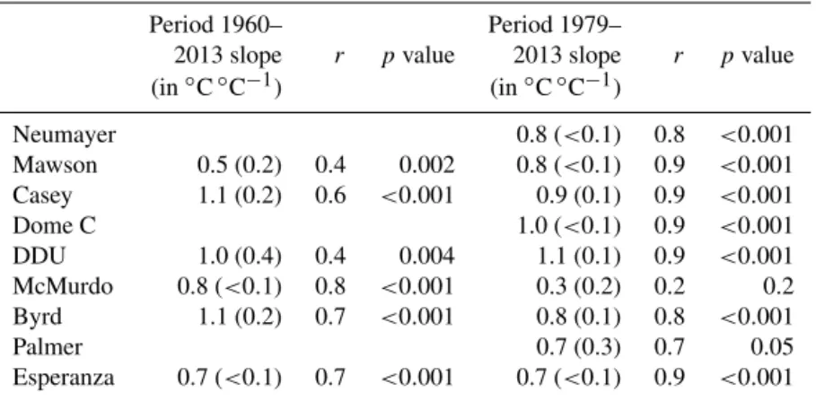
re-Table 2.Linear relationship between surface temperatures (in◦C) from station instrumental records and ECHAM5-wiso outputs (in◦C) over the period 1960–2013 and 1979–2013: the slope (in◦C◦C−1), the correlation coefficient (noted as “r”), and the p value. Data are not reported for 1960–2013 for stations for which records only cover the second period (1979–2013). Numbers in brackets correspond to standard errors.
Period 1960– Period 1979–
2013 slope r pvalue 2013 slope r pvalue (in◦C◦C−1) (in◦C◦C−1) Neumayer 0.8 (<0.1) 0.8 <0.001 Mawson 0.5 (0.2) 0.4 0.002 0.8 (<0.1) 0.9 <0.001 Casey 1.1 (0.2) 0.6 <0.001 0.9 (0.1) 0.9 <0.001 Dome C 1.0 (<0.1) 0.9 <0.001 DDU 1.0 (0.4) 0.4 0.004 1.1 (0.1) 0.9 <0.001 McMurdo 0.8 (<0.1) 0.8 <0.001 0.3 (0.2) 0.2 0.2 Byrd 1.1 (0.2) 0.7 <0.001 0.8 (0.1) 0.8 <0.001 Palmer 0.7 (0.3) 0.7 0.05 Esperanza 0.7 (<0.1) 0.7 <0.001 0.7 (<0.1) 0.9 <0.001
analyses. We note that mean values and the amplitude of inter-annual variations are different for ECHAM5-wiso and ERA (not shown), as expected from different model physics despite the nudging technique. This finding has led us to restrict, as far as possible, the subsequent analysis of the ECHAM5-wiso outputs to the period 1979–2013.
For this period marked by small temperature variations, we note that the correlation coefficient between data and model outputs (Table 2) is very small for McMurdo (r = 0.2) and rather small for Vostok (r = 0.6), questioning the ability of our simulation to resolve the drivers of inter-annual tempera-ture variability at these locations. We observe that the model reproduces the amplitude of inter-annual variations, with a tendency to underestimate the variations as shown by model– data slopes from 0.6 to 1◦C per◦C. As a result, ECHAM5-wiso underestimates the magnitude of inter-annual temper-ature variability for these central regions of the West and East Antarctic Ice Sheet. It will therefore be important to test whether similar caveats arise for water isotopes.
3.1.2 Comparison with GLACIOCLIM database accumulation
For each grid cell in which at least one stake record is avail-able, we have calculated the ratio of the P-E values (which we use as a surrogate for accumulation) simulated by ECHAM5-wiso to the averaged SMB estimate for that grid region based on stake measurements (Fig. 4a). Due to the limited num-ber of grid cells containing SMB data points from 1979 to 2013 (100 cells) located almost only on the East Antarctic Ice Sheet, we have decided to use the dataset covering the entire twentieth century (521 cells) spread over the continent.
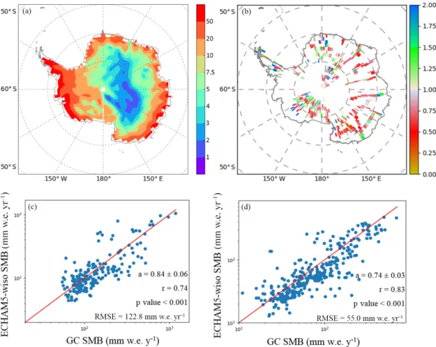
The spatial distribution of SMB is well captured by ECHAM5-wiso, with decreasing SMB values from the coast to the interior plateau (Fig. 4a). However, the model quan-titatively shows some discrepancies when compared with
the GC database. The area-weighted (by the model grid cells) mean GC SMB is 141.3 mm w.e. yr−1, while the sim-ulated area-weighted mean P-E over the same model grid is 126.6 mm w.e. yr−1. This underestimation covers 69.7 % of the compared areas. The 30.3 % remaining areas asso-ciated with an overestimation of the model are located in sparse regions like in the north of the plateau and over coastal areas (Fig. 4b). Note that the low P-E rates over the plateau (75 mm w.e. yr−1, see Fig. 4a) counterbalance the local overestimation at the coast, supporting the abil-ity of ECHAM5-wiso to resolve the integrated surface mass balance for the Antarctic ice sheet. Figure 4c and d con-firm the global underestimation by the model, with slopes of simulated P-E against GC SMB lower than 1. This as-pect is emphasised for elevations higher than 2200 m a.s.l. (r = 0.74 and rmse = 122.8 mm w.e. yr−1for elevation lower than 2200 m a.s.l., and r = 0.83 and rmse = 55 mm w.e. yr−1 for elevations higher than 2200 m a.s.l., with “r” the cor-relation coefficient, and “RMSE” the root mean square er-ror). The correlation coefficient (considering all elevations) is 0.79, reflecting the non-homogenous bias over the whole continent. This can be due first to a failure in the represen-tativity of SMB spatial variability when averaging GC data within ECHAM5-wiso grid cells due to a too-small number of point measurements. Second, the model grid resolution may be too coarse to reproduce coastal topography and thus the associated amounts of precipitation. Finally, several key processes such as blowing snow erosion and deposition are not taken into account in the model. For instance, the lowest value from the GC database is −164 mm w.e. yr−1, measured at the Bahia del Diablo glacier, a small glacier covering im-portant elevation ranges in a narrow spatial scale between the front and the summit. It was the only one within the corre-sponding model grid cell, so the resulting GC value within this grid cell could not be representative of the model scale,
Figure 4.Comparison of the GLACIOCLIM (hereafter and noted in the plots as “GC”) SMB database averaged within the ECHAM5-wiso grid cells and the SMB (i.e. precipitation–evaporation) simulated by the model, with the spatial distribution of the accumulation (a) as simulated by the model (in cm w.e. yr−1), (b) the ratio of the ECHAM5-wiso annual accumulation (precipitation minus evaporation) to the GC averaged SMB (no unit), and GC-averaged SMB values against SMB values simulated by the model (blue dots) associated with the corresponding linear relationships (red solid line); displayed at the logarithm scale for elevation ranges of 0–2200 m a.s.l. (with the upper limit excluded) (c) and 2200–4000 m a.s.l. (d).
and the simulated P-E value is not representative of this small glacier-wide value.
When considering the whole Antarctic grounded ice sheet, the area-weighted P-E simulated by the model amounts to 164.4 mm w.e. yr−1. This value falls within the highest values of the 11 simulations displayed by Monaghan et al. (2006), varying from 84 to 188 mm w.e. yr−1. However, the high range of values between the different simulations illustrates the uncertainties related to the SMB model, mainly due to model resolution, which is crucial to reproducing the impact of topography on precipitations and to non-resolved phys-ical processes (e.g. drifting snow transport, including the erosion, deposition, and sublimation of drifting snow parti-cles, and clouds microphysics; Favier et al., 2018). More-over, this simulated value is very close to the best estima-tions of Antarctic grounded ice sheet SMB, which range be-tween 143.4 (Arthern et al., 2006) and 160.8 mm w.e. yr−1 (Lenaerts et al., 2012). This simulated value is also very close to the one obtained by Agosta et al. (2013) for the LMDZ4
model over the period 1981–2000 (160 mm w.e. yr−1), but slightly lower than with the SMHiL model forced by LMDZ4 (189 mm w.e. yr−1).
To conclude, although the ECHAM5-wiso simulation presented in this study has a relatively coarse resolu-tion (110 km × 110 km compared to 15 km × 15 km for the SMHiL model forced by LMDZ4) and does not resolve processes contributing in the SMB (e.g. drifting snow pro-cesses), the P-E outputs are realistic products when com-pared with SMB data.
3.2 Comparison with water stable isotope data
Limited by the availability of the data, we could only study model skills with respect to spatio-temporal patterns, includ-ing seasonal and inter-annual variations, and the simulated relationships between δ18O and temperature. We have also extended the model–data comparison to the second-order pa-rameter, d.
Table 3.Comparison between measurements from precipitation samples and ECHAM5-wiso simulated precipitation isotopic composition for grid cells closest to the sampling locations over the same period as the data (at daily or monthly scale when the name of the station is associated with an asterisk). We report the mean value ± the standard deviation for δ18O (in ‰) and for temperature (◦C).
Number Data Model
of points Temperature (◦C) δ18O (‰) Temperature (◦C) δ18O (‰) Rothera∗ 194 −12.9 ± 3.4 −4.0 ± 4.1 −12.3 ± 6.4 −6.7 ± 5.3 Vernadsky∗ 372 −9.9 ± 3.1 −3.1 ± 3.6 −13.5 ± 6.0 −9.0 ± 7.2 Halley∗ 552 −22.0 ± 5.5 −18.7 ± 1.7 −25.7 ± 7.1 −20.1 ± 7.6 Marsh∗ 19 −12.1 ± 4.1 −3.4 ± 3.0 −10.4 ± 5.1 −4.2 ± 3.6 Dome F 351 −61.3 ± 10.8 −54.7 ± 12.6 −58.3 ± 12.2 −53.4 ± 12.1 Dome C 501 −58.0 ± 8.6 −55.2 ± 13.8 −59.6 ± 17.4 −52.9 ± 10.9 DDU 19 −18.0 ± 3.8 −23.4 ± 5.1 −21.3 ± 7.8 Neumayer 336 −20.8 ± 6.6 −13.4 ± 8.0 −21.3 ± 7.9 −15.8 ± 7.9
3.2.1 δ18O time-averaged values and inter-annual variability
The model–data difference of the time-averaged values is positive for 88 % of all grid cells, suggesting a system-atic underestimation of isotopic depletion by ECHAM5-wiso (Fig. 5a). The few areas for which ECHAM5-wiso overes-timates the isotopic depletion are restricted to coastal re-gions. This pattern is coherent with the temperature anoma-lies: ECHAM5-wiso produces too-low isotopic values where ECHAM5-wiso has a cold bias, likely causing too-strong dis-tillation towards coastal areas and too-high isotopic values inland, where the warm bias limits the distillation strength. The statistical distribution of model–data δ18O differences (not shown) shows a wide range but an interquartile range (50 % of all values) of 1.4 to 3.9 ‰, which is therefore within 1.3 ‰ of the median. We conclude that, beyond the system-atic offset linked to climsystem-atic biases, ECHAM5-wiso correctly captures the spatial gradient (continental effect) of annually averaged δ18O data. These results also suggest that the spa-tial distribution of annual mean δ18O values from shallow ice cores is driven by transport and condensation processes well resolved by ECHAM5-wiso, probably with secondary effects of non-resolved processes such as snow drift, wind erosion, and snow metamorphism. The largest deviations are encountered in coastal regions, where the model resolution is too low to correctly resolve topography, advection, and boundary layer processes (e.g. small-scale storms, katabatic winds). Katabatic winds also have the potential to enhance ventilation-driven post-deposition processes (Waddington et al., 2002; Neumann and Waddington, 2004).
δ18O inter-annual standard deviation is underestimated by the model for 92 % of the 179 grid cells in which this com-parison can be performed (Fig. 5b).The interquartile range of the ratio between the simulated and observed standard devi-ation varies from 0.4 to 0.6 (not shown), with an underesti-mation by a factor of 2 for about 50 % of the grid cells. No such underestimation of inter-annual standard deviation was identified for the simulated temperature.
We now focus on our model–data comparison of precipi-tation data. Both precipiprecipi-tation isotopic composition and tem-perature measurements are available for only eight locations and for short time periods (Table 3). These data evidence the altitude and continental effect with increased isotopic depletion from Vernadsky (averaged δ18O of −9.9 ‰) to Dome F (averaged δ18O of −61.3 ‰). For five out of the eight records, the isotopic depletion is stronger in ECHAM5-wiso than observed (Dome C included). The observations de-pict an enhanced inter-daily δ18O standard deviation for in-land sites, from 3.1 at Vernadsky to 10.8‰ at Dome F. The simulated δ18O inter-daily standard deviation is 1.1 to 3.8 times larger than observed, ranging from 5.1 to 19.2 ‰. For the exact same time period corresponding to the short pre-cipitation isotopic records, ECHAM5-wiso simulates colder than observed temperatures at all stations but Dome F and Dome C, i.e. over the plateau. This finding is consistent with results from ice core records reported previously and con-sistent with the isotopic systematic biases. From this limited precipitation dataset, there is no systematic relationship be-tween model biases for temperature (mean value or standard deviation) or for δ18O in contrast with the outcomes of the model–data comparison using the whole dataset, including surface snow. At Dome C, ECHAM5-wiso underestimates the standard deviation of temperature, but strongly overesti-mates the standard deviation of δ18O.
As a conclusion, while δ18O time-averaged model–data bi-ases are consistent with temperature bibi-ases using the whole dataset, no systematic relationships emerge between model biases for temperature and δ18O measured in precipitation.
3.2.2 δ18O seasonal amplitude
High-resolution δ18O data allow us to explore seasonal varia-tions. This includes 18 ice core records with sub-annual reso-lution, four IAEA/GNIP monthly precipitation datasets, and four daily precipitation monitoring records.
In order to quantify post-deposition effects in ice cores, we calculated the ratio of the first three seasonal amplitudes by
Figure 5.Maps displaying model–data comparisons for δ18O time-averaged values (a) and inter-annual standard deviations (b). Back-grounds correspond to ECHAM5-wiso simulations over the period 1979–2013, while signs correspond to the model–data comparison. For the time-averaged values, the comparison consists of calculat-ing the model–data differences. Red “+” symbols indicate a posi-tive model–data difference, while blue “−” symbols correspond to a negative model–data difference. For the inter-annual standard de-viations, the comparison consists of calculating the ratio of the sim-ulated value to the corresponding grid cell data. Red “+” symbols indicate a ratio higher than 1, while blue “−” symbols correspond to a model / data ratio lower than 1.
using the mean seasonal amplitude in sub-annual ice cores (See Table S2 in the Supplement). We find a mean ratio of 1.40 ± 0.47. We explored whether this ratio was related to annual accumulation rates (see Fig. S3 in the Supplement), without any straightforward conclusion. We also observe that five ice cores depict a ratio lower than 1, including one with a mean yearly accumulation of 15 cm w.e. yr−1, a feature which may arise from inter-annual variability in the
precip-Figure 6. Maps displaying model–data comparisons for d time-averaged (in ‰, a) values and inter-annual standard deviations (in ‰, b). Backgrounds correspond to ECHAM5-wiso simulations over the period 1979–2013, while signs correspond to the model– data comparison. For the time-averaged values, the comparison con-sists of calculating the model–data differences. Red “+” symbols indicate a positive model–data difference, while blue “−” symbols correspond to a negative model–data difference. For the inter-annual standard deviation, the comparison consists of calculating the ratio of the simulated value to the corresponding grid point data. Red “+” symbols indicate a ratio higher than 1, while blue “−” symbols correspond to a model / data ratio lower than 1.
itation seasonal amplitude or in post-deposition processes. This empirical analysis shows that a loss of seasonal ampli-tude due to post-deposition processes is likely in most cases, with an average loss of the seasonal amplitude of approxi-mately 70 % compared to the amplitude recorded in the up-per part of the firn cores (first 3 years).
We have calculated the mean of the δ18O annual amplitude (i.e. maximum–minimum values within each year) in ice core records (triangles in Fig. 7a) and the mean seasonal
ampli-Figure 7.Average seasonal amplitude of precipitation δ18O (a) and d (b) (in ‰) simulated by ECHAM5-wiso (colour shading) over the period 1979–2013 and calculated from precipitation data (cir-cles) and ice core records (triangles) over their respective available periods.
tude of precipitation time series (circles in Fig. 7a) for com-parison with ECHAM5-wiso outputs (Fig. 7, Table 4). Unfor-tunately, a too-small number of measurements (19 daily mea-surements) were monitored at DDU, preventing the represen-tation of the full seasonal cycle. The data depict the largest seasonal amplitude in the central Antarctic Plateau, reach-ing up to 25.9 ‰ at Dome F. ECHAM5-wiso underestimates the seasonal amplitude (by 14 to 69 %) when compared to precipitation data, but overestimates the seasonal amplitude when compared to ice core data (from 11 to 71 %). The over-estimation when comparing with ice core data is consistent with the attenuation of signal by post-deposition effects (as previously mentioned) rather than a model bias.
The simulated mean seasonal δ18O amplitude increases gradually from coastal regions to central Antarctica (more
Table 4.δ18O mean seasonal amplitude (in ‰) calculated for pre-cipitation and sub-annual ice core data, as well as simulated by ECHAM5-wiso for the same time period as the data. The time res-olution used in the model corresponds to the time resres-olution of the precipitation data and to the annual scale for the ice core data (i.e. yearly averages based on daily precipitation isotopic composition weighted by the amount of daily precipitation). The data type is identified as 1 for precipitation samples and 2 for ice core data.
Station Type δ18O ECHAM5-wiso observed averaged over amplitude the observed (‰) period (‰) Rothera 1 4.1 1.9 Vernadsky 1 4.1 2.3 Halley 1 13.2 6.7 Marsh 1 10.4 7.3 Dome F 1 25.9 15.3 Dome C 1 20.1 13.5 DDU 1 6.1 3.7 Neumayer 1 12.8 7.9 USITASE-1999-1 2 7.2 13.2 USITASE-2000-1 2 4.8 10.6 USITASE-2000-2 2 7.7 10.4 USITASE-2000-4 2 4.0 12.0 USITASE 2000-5 2 5.2 13.7 USITASE-2000-6 2 2.8 14.2 USITASE-2001-1 2 7.3 9.4 USITASE-2001-2 2 7.3 12.0 USITASE-2001-4 2 6.2 8.9 USITASE-2001-5 2 6.8 9.0 USITASE-2002-1 2 4.2 12.2 USITASE-2002-2 2 6.3 10.7 USITASE-2002-4 2 5.3 13.8 NUS 08-7 2 3.4 16.6 NUS 07-1 2 2.1 14.8 WDC06A 2 4.0 10.8 IND25 2 5.3 12.6 GIP 2 15.1 16.8
than 15 and up to 25 ‰ for some areas; Figs. 7a and 8c, solid lines). The model–data comparison suggests that this pattern is correct and that the model may underestimate the inland seasonal amplitude. As previously reported for annual mean values, systematic offsets are also identified for sea-sonal variations, with a systematic overestimation of monthly isotopic levels inland (e.g. for Dome C and Dome F) and a systematic underestimation on the coast (e.g. for Vernadsky and Halley). The model–data mismatch is largest during lo-cal winter months.
Minima are observed and simulated in winter (May– September) at most locations, except for Rothera and Ver-nadsky where the data show a minimum in July but the model produces a minimum in late autumn (April). Maximum val-ues are observed and simulated in local summer (December–
Figure 8. Average seasonal cycles from precipitation data over the available period (dashed lines with points) and simulated by the ECHAM5-wiso model over the period 1979–2013 (solid lines) of the temperature (in◦C) (a), the precipitation (in mm w.e. yr−1), the pre-cipitation δ18O (in ‰) (c) and the deuterium excess (in ‰) (d). Data are shown for different durations depending on sampling, while model results are shown for the period 1979–2013. The number of points used for the observations is given in Table 3.
January); a secondary maximum is also sometimes observed and simulated in late winter (August–September). Data from Marsh station show maxima in January, April, and August, whereas the model only produces a single summer maximum value.
In summary, we report no systematic bias of the seasonal temperature amplitude (Fig. 8a). The seasonal pattern for the temperature is similar compared to δ18O, with minima in winter and the largest model–data mismatch in winter. Sec-ondary minima or maxima cannot be discussed with confi-dence, as they have low amplitudes. We also highlight that model–data offsets are larger in winter. Note that precipita-tion and d seasonal cycles are described in Sect. 3.2.4.
3.2.3 δ18O–T relationships
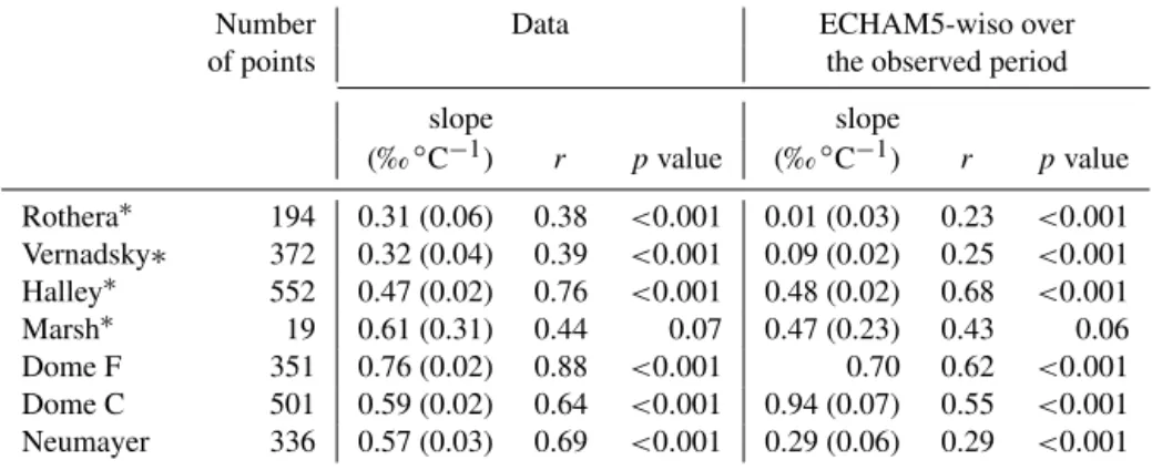
Table 5 reports the temporal δ18O–T relationships estab-lished from precipitation and temperature observations and those simulated by ECHAM5-wiso. This calculation is based on daily or monthly values (depending on the sampling
res-olution) and includes seasonal variations. The data display significant linear relationships for all sites but Marsh (p value = 0.07), with an increased strength of the correlation coefficient from the coast (e.g. r = 0.38 at Rothera) to the East Antarctic Plateau (e.g. r = 0.88 at Dome F). The low-est slopes are identified in the peninsula region, with a mean slope of 0.32 ‰◦C−1for Rothera and Vernadsky, while the highest slopes occur over the East Antarctic Plateau, with a mean slope of 0.68 ‰◦C−1for Dome C and Dome F. These temporal slopes appear mostly lower than the spatial slopes and those expected from a Rayleigh distillation with a single moisture source (typically 0.8 ‰◦C−1).
In the ECHAM5-wiso model, as for the data, the simu-lated isotope–temperature relationship is statistically signifi-cant for all sites but Marsh (p value = 0.06). However, corre-lation coefficients are very small for Rothera and Vernadsky, which are thus excluded from further analyses. In the simula-tion, correlation coefficients are the highest for Halley, Dome C, and Dome F (up to 0.55) and the lowest for Neumayer (as
Table 5.Slope (in ‰◦C−1), correlation coefficient, and p value of the δ18O–temperature linear relationship from precipitation measure-ments over the available period at daily or monthly (when the name of the station is associated with an asterisk) scale, depending on the time resolution of the data, and from the ECHAM5-wiso model over the observed period at the time resolution of the data. Numbers in brackets correspond to the standard errors.
Number Data ECHAM5-wiso over
of points the observed period
slope slope (‰◦C−1) r pvalue (‰◦C−1) r pvalue Rothera∗ 194 0.31 (0.06) 0.38 <0.001 0.01 (0.03) 0.23 <0.001 Vernadsky∗ 372 0.32 (0.04) 0.39 <0.001 0.09 (0.02) 0.25 <0.001 Halley∗ 552 0.47 (0.02) 0.76 <0.001 0.48 (0.02) 0.68 <0.001 Marsh∗ 19 0.61 (0.31) 0.44 0.07 0.47 (0.23) 0.43 0.06 Dome F 351 0.76 (0.02) 0.88 <0.001 0.70 0.62 <0.001 Dome C 501 0.59 (0.02) 0.64 <0.001 0.94 (0.07) 0.55 <0.001 Neumayer 336 0.57 (0.03) 0.69 <0.001 0.29 (0.06) 0.29 <0.001
low as 0.29). The slope is the lowest at Neumayer, with a value of 0.29 ‰◦C−1, increases at Halley with a value of 0.48‰◦C−1, and is the highest over the plateau with values of 0.70 ‰◦C−1at Dome C and up to 0.94 ‰◦C−1at Dome F.
To summarise, ECHAM5-wiso tends to underestimate the strength of the isotope–temperature relationship, but cor-rectly simulates a larger strength of the correlation in the central Antarctic Plateau compared to coastal regions. There are significant differences in the isotope–temperature slopes for both coastal and central plateau locations. While there is some agreement (e.g. for Dome F and Halley), the model also produces non-realistic slopes, with a much larger slope than observed at Dome C, for instance.
3.2.4 The δD–δ18O relationship and d patterns
The δ18O–δD linear relationship is expected to be affected by different kinetic fractionation processes, for instance those associated with changes in evaporation conditions. We first compare the δ18O–δD linear relationship in the available pre-cipitation and ice core data and simulated by ECHAM5-wiso (Table 6). Significant correlation is observed for all observa-tional datasets but Marsh, as expected from meteoric sam-ples, assuming correct preservation of samples and accurate isotopic measurements. We stress that the smallest correla-tion coefficient is identified at Vernadsky (r = 0.96), suggest-ing potential artefacts for this record. In the observations, the δD–δ18O slope varies across regions. While slopes higher than for the global meteoric waterline (i.e. > 8 ‰ ‰−1) are identified at DDU and in Dronning Maud Land, lower slopes are identified in the Antarctic Peninsula (6.6 to 7.0 ‰ ‰−1) and in the central East Antarctic Plateau (6.5 and 6.4 ‰ ‰−1 at Dome C and Dome F, respectively). In the model, out-puts also display significant linear relationships. They show higher values of the slope than observed in the Antarctic
Peninsula, at DDU, and at Dome F and lower than observed for the other regions, including Dome C. These results ap-pear coherent with associated coastal versus inland tempera-ture and isotopic distillation biases.
Figure 6 compares the spatial patterns of the d time-averaged model–data difference (characterised at 293 grid cells in our database; see Fig. 6a), and the situation is con-trasted with 50 % of positive and negative differences. We can identify systematic trends, with an underestimation of the mean d levels in ECHAM5-wiso for the central East Antarctic Plateau and the peninsula and an overestimation above Victoria Land (Fig. 6a). Due to the temperature de-pendency of equilibrium fractionation coefficients leading to a gradual deviation from the meteoric waterline (calculated at the global scale, at which a coefficient of 8 results from the average equilibrium fractionation coefficients), d increases when temperature decreases (Masson-Delmotte et al., 2008; Touzeau et al., 2016). For central Antarctica, the d bias is thus consistent with the warm bias and the lack of isotopic depletion. The upper and lower quartiles of the model–data differences range within ±1.5 ± 0.1 ‰, suggesting that the model outputs remain close to those observed.
The d pattern is similar to that of δ18O: ECHAM5-wiso underestimates the d standard deviation for 90 % of grid cells, with an interquartile range comparable to the one for the ratio of standard deviations for δ18O (Fig. 6b). Table 7 displays the comparison of the statistics between d in the ob-servations and in ECHAM5-wiso. In the obob-servations, the time-averaged d is particularly low in the peninsula (−3.6 to 8.6 ‰), intermediate in the coastal regions of Dronning Maud Land, Victoria Land, and Adélie Land (4.4 to 8.6 ‰), and very high in the central Antarctic Plateau (up to 17.5 ‰ for Dome C). Lower coastal values and higher inland values are captured by ECHAM5-wiso, albeit with large offsets for each site reaching several per mille. These findings are con-sistent with the map showing the time-averaged precipitation
Table 6.Slope (in ‰ ‰−1), correlation coefficient, and p value of the δ18O–δD linear relationship from precipitation measurements (top of the table) and ice core data (bottom of the table) over the available period at daily or monthly scale (identified with an asterisk) and from the ECHAM5-wiso model over the observed period at the time resolution of the data for the precipitation and at the annual scale for the ice core data. Numbers in brackets correspond to the standard errors.
Number Observations ECHAM5-wiso
of points slope r pvalue slope r pvalue
(‰ ‰−1) (‰ ‰−1) Rothera∗ 194 7.0 (<0.1) 9.81 × 10⁻¹ <0.001 7.9 (<0.1) 9.97 × 10⁻¹ <0.001 Vernadsky∗ 372 6.6 (<0.1) 9.62 × 10⁻¹ <0.001 7.8 (0) 9.96 × 10⁻¹ 0 Halley∗ 552 7.8 (0) 9.91 × 10⁻¹ 0 7.8 (<0.1) 9.95 × 10⁻¹ <0.001 Marsh∗ 19 7.1 (<0.1) 9.80 × 10⁻¹ <0.001 8.0 (<0.1) 9.94 × 10⁻¹ <0.001 Dome F 351 6.4 (<0.1) 9.92 × 10⁻¹ <0.001 7.3 (<0.1) 9.91 × 10⁻¹ <0.001 Dome C 501 6.5 (0) 9.89 × 10⁻¹ 0 6.3 (<0.1) 9.73 × 10⁻¹ <0.001 DDU 19 8.5 (<0.1) 9.92 × 10⁻¹ <0.001 9.0 (<0.1) 9.86 × 10⁻¹ <0.001 Neumayer 336 7.9 (<0.1) 9.90 × 10⁻¹ <0.001 7.8 (<0.1) 9.98 × 10⁻¹ <0.001 NUS 08-7 256 8.6 (<0.1) 9.96 × 10⁻¹ <0.001 8.0 (<0.1) 9.95 × 10⁻¹ <0.001 NUS 07-1 118 8.3 (<0.1) 9.94 × 10⁻¹ <0.001 7.6 (<0.1) 9.94 × 10⁻¹ <0.001 WDC06A 540 8.2 (0) 9.95 × 10⁻¹ 0.00 8.1 (<0.1) 9.98 × 10⁻¹ <0.001 IND25 349 8.2 (<0.1) 9.82 × 10⁻¹ <0.001 7.8 (<0.1) 9.94 × 10⁻¹ <0.001 GIP 495 7.8 (0) 9.90 × 10⁻¹ 0 8.3 (<0.1) 9.98 × 10⁻¹ <0.001
d simulated by ECHAM5-wiso over the period 1979–2013 (Fig. 6a), with very low coastal values (close to zero) and increasing values towards the interior of Antarctica, reach-ing values higher than 16 ‰ on the plateau. ECHAM5-wiso mainly underestimates the d intra-annual standard deviation for 10 sites out of 15 (Table 7 and Fig. 6b).
Figure 8d depicts the mean d seasonal patterns of the pre-cipitation data and corresponding model outputs. The data show different patterns from one location to another. While d measured at Neumayer, Halley, and Rothera displays a maximum in autumn (March–April), it appears in late au-tumn (May) at Marsh and in winter (June–August) at Ver-nadsky. Maxima for central stations are observed later, in May–July for Dome C and July–September for Dome F. In short, most coastal areas are associated with a maximum d in autumn, while central areas are associated with a later maximum d, i.e. in winter or late winter, that is thus in anti-phase with δ18O and temperature. The seasonal amplitude in-creases from the coast to the plateau. In the model, for central areas, a first d maximum is simulated earlier than observed (February–March for Dome F and May–June for Dome C), followed by a second maximum in late winter (August for Dome F and September for Dome C). For coastal areas, the amplitude of the simulated d signal is too small to unequivo-cally estimate the timing of the maximum. Note the very low value simulated at DDU in July, which appears to be an out-lier when comparing this value with the average modelled d value for all days in August 1973 (+5.9 ‰). No link emerges between the modelled seasonal patterns in d and in tempera-ture (Fig. 8a), accumulation (Fig. 8b), or δ18O (Fig. 8c).
Table 7.Mean value ± standard deviation (in ‰) of sub-annual d in observational time series at daily or monthly scale (identified with an asterisk) for the precipitation and for the ice core data and simu-lated d by ECHAM5-wiso for the same time period as the observa-tions for precipitation and at the annual scale for the ice core. Mean values which are overestimated by ECHAM5-wiso are written in italic.
Data (‰ ) ECHAM5-wiso over the observed period (‰) Rothera∗ −1.1 ± 5.7 2.9 ± 1.5 Vernadsky∗ −1.5 ± 7.0 3.5 ± 1.5 Halley∗ 5.77 ± 6.1 2.8 ± 1.9 Marsh∗ 8.6 ± 7.0 2.4 ± 1.7 Dome F 17.4 ± 19.5 15.3 ± 14.2 Dome C 17.5 ± 15.2 14.2 ± 24.3 DDU 5.9 ± 4.5 2.8 ± 9.5 Neumayer 8.7 ± 5.6 2.4 ± 4.7 NUS 08-7 5.0 ± 2.7 6.6 ± 1.0 NUS 07-1 5.8 ± 2.3 7.0 ± 1.1 WDC06A 3.6 ± 1.5 4.5 ± 0.5 IND25 4.4 ± 19.2 4.1 ± 0.9 GIP 6.0 ± 4.4 2.1 ± 0.9
Finally, Table 8 reports the d mean seasonal amplitude val-ues for the precipitation data and ice core records, as well as for the model outputs covering the observation. They clearly show an increase in d seasonal amplitude from the coast to the plateau (see also Fig. 7b), with values varying from 6.7 at
Table 8.The d mean seasonal amplitude (in ‰) calculated for pre-cipitation at daily or monthly scale (identified with an asterisk) and sub-annual ice core data, as well as simulated by ECHAM5-wiso for the same time period as each record. The data type is identified as 1 for precipitation samples and 2 for ice core records. Ampli-tude values that are overestimated by ECHAM5-wiso are written in italic.
Station Type Observed ECHAM5-wiso amplitude outputs for the observed period (‰) (‰) Rothera∗ 1 10.7 3.1 Vernadsky∗ 1 11.8 2.1 Halley∗ 1 6.7 3.8 Marsh∗ 1 25.8 4.5 Neumayer 1 7.3 5.3 Dome F 1 40.1 12.2 Dome C 1 41.0 25.4 NUS 08-7 2 3.5 14.0 NUS 07-1 2 1.9 15.8 WDC06A 2 1.0 16.5 IND25 2 2.3 11.7 GIP 2 17.8 6.9
Halley to 41 ‰ at Dome C. ECHAM5-wiso systematically underestimates the d mean seasonal amplitude when com-pared with precipitation data, while it systematically over-estimates it when compared with ice core data (from 9.4 to 15.5 ‰), with the exception of the GIP ice core. Again, we cannot rule out a loss of amplitude in ice core data compared to the initial precipitation signal due to the temporal resolu-tion and post-deposiresolu-tion effects.
3.3 Strength and limitations of the ECHAM5-wiso model outputs
The isotopic model–data time-averaged biases appear coher-ent with temperature. A warm bias over ccoher-entral East Antarc-tica and a cold bias over coastal regions lead to a too-low and too-strong isotopic depletion, respectively. Temperature and distillation biases also explain the underestimation of d above the central East Antarctic Plateau.
However, some characteristics are not explained by model skills for temperature. At sub-annual timescales, ECHAM5-wiso always overestimates the standard deviation of δ18O in precipitation (Table 3), but results for d are mixed (Table 7). ECHAM5-wiso always underestimates the seasonal ampli-tude of δ18O and d in precipitation but always overestimates the seasonal amplitude of δ18O and d in firn–ice cores (Ta-bles 4 and 8). Differences between the model and firn–core data are at least partially due to diffusion processes, but no clear reason can be given for the other isotopic biases.
We do not find any clear link between other model biases for d and those for temperature or δ18O.
Sampling Antarctic snowfall remains challenging (Fujita and Abe, 2006; Landais et al., 2012; Schlosser et al., 2016; Stenni et al., 2016). Sampling is likely to fail to capture small events and may also collect surface snow transported by winds or hoar. Snow samples may undergo sublimation before collection. The fact that ECHAM5-wiso appears to overestimate the variability of precipitation isotopic com-position may be related to an improper characterisation of the full day-to-day variability of real-world precipitation from daily precipitation sampling. Alternatively, this feature may also arise from a lack of representation of small-scale processes (boundary layer processes, wind characteristics, snow–atmosphere interplays) in ECHAM5-wiso. These pro-cesses may contribute to a local source of Antarctic moisture (through local recycling), reducing the influence of large-scale moisture transport (resolved by ECHAM5-wiso nudged to reanalyses) on the isotopic composition of precipitation and its day-to-day variability.
Caveats also limit the interpretation of the comparison of ECHAM5-wiso precipitation outputs with surface snow or shallow ice core data. Such records are potentially affected by post-deposition processes, such as wind scoring, erosion, snow metamorphism between precipitation events, and dif-fusion.
Our apparently contradictory findings for model–data comparisons with respect to inter-annual variations (from ice cores) and inter-daily variations (from precipitation data) call for more systematic comparisons between δ18O records of precipitation and ice cores at the same locations over several years.
4 Use of ECHAM5-wiso outputs for the interpretation of ice core records
In this section, we use the model outputs to help in the in-terpretation of ice core data: we quantify the inter-annual isotope–temperature relationships (Sect. 4.2) and charac-terise the spatial distribution of seasonal δ18O–d phase lag. Based on the confidence we can have in the model for each of the seven aforementioned regions (see Sect. 1 and Fig.1), we formulate recommendations for the future use of ECHAM5-wiso outputs (Sect. 4.3).
4.1 Spatial and temporal isotope–temperature relationships
First, we use ECHAM5-wiso to investigate spatial δ18O– temperature relationships (Fig. 9a and b) and then inter-annual (Fig. 9c and d) and seasonal relationships (Fig. 9e and f). For spatial relationships, the strength of the linear correlation coefficient is higher than 0.8. The spatial slope shows regional differences. It is generally smaller near the coasts (less than 0.8 ‰◦C−1), with the exception of
Dron-Figure 9.Linear analysis of annual ECHAM5-wiso outputs from 1979–2013 for the temporal δ18O–temperature relationship (using the 2 m temperature and the precipitation-weighted δ18O). Maps show the slope of the linear regression (‰◦C−1) at the right side (a, c, e) and the correlation coefficient at the left side (b, d, f). The upper plots use outputs at the spatial scale (a, b), the middle plots at the inter-annual scale (c, d), and the lower plots at the seasonal scale (e, f). Areas where the results of the linear analysis are not significant are hatched (p value > 0.05).
ning Maud Land, and increases at elevations higher than 2500 m a.s.l., with values above 1.2 ‰◦C−1in large areas. Furthermore, ECHAM5-wiso simulates the spatial hetero-geneity of the gradient in the central East Antarctic Plateau around Dome C, Dome A, and Dome F. Such variability may arise from the simulated intermittency of precipitation and from differences in condensation versus surface temperature. At the inter-annual scale (Fig. 9c and d), results are not significant for large areas encompassing the Dronning Maud Land region, the Antarctic Peninsula, the
Transantarc-tic Mountain region, the Ronne and Filchner ice shelf re-gions, part of Victoria Land, and along the Wilkes Land coast. For the whole continent, the correlation coefficient varies between 0.5 and 0.6 (with few values reaching 0.6 at the upper limit and 0.3 at the lower limit). Where correlations are significant, the inter-annual δ18O–temperature slope in-creases from the coasts (0.3 to 0.6 ‰◦C−1) to the inland re-gions, where it can exceed 1 ‰◦C−1for some high-elevation locations. The low correlation may be due to the small range of mean annual temperature over the period 1979–2013 and
is not necessarily indicative of a weak sensitivity to temper-ature change.
Finally, at the seasonal scale, results are significant almost over the whole continent (with the exception of two little ar-eas in the peninsula and East Antarctica) and the correlation coefficients are equal to 1 everywhere but along the coastal regions in the Indian Ocean sector, where the correlation co-efficient can decrease down to 0.75. Slopes are lower than for spatial and inter-annual relationships, with values from 0.0 to 0.3 ‰◦C−1along the coast (higher over Dronning Maud Land and the Ross Ice Shelf region), around 0.5 ‰◦C−1 in-land for altitudes lower than 2500 m a.s.l. (with the exception of lower values above the Transantarctic Mountains), and up to 0.8 ‰◦C−1over the East Antarctic Plateau.
To conclude, the coherent framework provided by the ECHAM5-wiso simulation covering the period 1979–2013 shows that annual δ18O and surface temperatures are only weakly linearly related in several areas. This suggests that the inter-annual variability of δ18O is controlled by other pro-cesses, for instance those associated with synoptic variabil-ity and changes in moisture source characteristics (Sturm et al., 2010; Steiger et al., 2017). Moreover, our results rule out the application of a single isotope–temperature slope for all Antarctic ice core records on the inter-annual timescale, and the seasonal isotope–temperature slope is not a surrogate for scaling inter-annual δ18O to temperature.
We have also used the simulation to explore linear rela-tionships between d and surface air temperature, without any significant results (not shown).
4.2 δ18O–d phase lag
Deuterium excess (d) has originally been interpreted as a proxy for relative humidity at the moisture source (Jouzel et al., 2013; Pfahl and Sodemann, 2014; Kurita et al., 2016). However, recent studies of Antarctic precipitation data com-bined with back-trajectory analyses did not support this inter-pretation (e.g. Dittmann et al., 2016; Schlosser et al., 2017), calling for further work to understand the drivers of sea-sonal d variations. The phase lag between d and δ18O was initially explored to identify changes in evaporation condi-tions (Ciais et al., 1995). In ECHAM5-wiso, this phase lag is calculated as the lag that gives the highest correlation co-efficient between d and δ18O (Fig. 10) using the mean sea-sonal cycle from monthly averaged values. If there were no seasonal change in moisture origin and climatic conditions during the initial evaporation process, one would expect d to be in anti-phase with δ18O due to the impact of conden-sation temperature on equilibrium fractionation. For regions with small seasonal amplitude in condensation temperature, a constant initial isotopic composition at the moisture source would imply a stable d year-round. In such regions, the sim-ulated phase lag likely therefore reflects seasonal changes in the d of the initial moisture source. The comparison with pre-cipitation data (Sect. 3.2.4) showed that ECHAM5-wiso had
low seasonal amplitude in coastal regions (Fig. 8d), mak-ing the discussion of seasonal maxima difficult. These com-parisons are also limited by the duration of the precipita-tion records. Here, we use the full simulaprecipita-tion (1979–2013) to investigate the phase lag between the mean seasonal cy-cle of d and δ18O. Clear spatial patterns are identified for the distribution of this phase lag (see Fig. 10). At intermedi-ate elevations (between 1000 and 3000 m a.s.l.), d seasonal variations occur in phase (within 2 months) with the sea-sonal cycle of δ18O (and surface air temperature). By con-trast, a phase lag of several months is identified over coastal areas and over the central East Antarctic Plateau. Along the Wilkes Land coast and the Dronning Maud Land region, the time lag is between 2 and 4 months below 1000 and 500 m a.s.l., respectively. Over the West Antarctic Ice Sheet, the phase lag is higher than 2 months below 500 m a.s.l. and can even reach 6 months (indicating an anti-phase between d and δ18O). Over the central East Antarctic Plateau (above 3000 m of elevation), the phase lag reaches several months again, especially near Dome C. Obtaining longer precipita-tion records and comparing the phase lag identified in pre-cipitation and surface snow records would be helpful to un-derstand whether post-deposition processes, which are not included in ECHAM5-wiso, affect this phase lag. The dif-ferent characteristics of seasonal d changes suggest differ-ent seasonal changes in moisture origin at coastal, interme-diate, and central plateau regions, supporting the identifica-tion of specific coastal versus inland regions to assess the isotope–temperature relationships. Note that the few avail-able datasets are in line with the simulation.
4.3 Recommendations for the different regions of Antarctica
In this section, we summarise our findings based on the model–data comparisons and the analysis of model outputs for the seven Antarctic regions selected by the Antarctica2k program, as shown in Fig. 1 (Stenni et al., 2017). The regions depend on geographical and climatic characteristics. Results from Sect. 3 were averaged over each region and are given in Table 9.
We first discuss the systematic model biases. The maxi-mum time-averaged model–data differences (3.8 and 2.6 ‰ for δ18O and d, respectively) are identified in the Weddell Sea area. Minimum time-averaged model–data differences occur in different regions for δ18O and d (Victoria Land and Dron-ning Maud Land, respectively).
For inter-annual standard deviation, the model–data mis-match is smallest for Victoria Land (ratio of 1.1 and 1.0 for δ18O and d, respectively). Results for δ18O show that the simulated inter-annual variability can be considered close to reality (model–data ratio higher than 0.7) only for Victoria Land and the plateau, acceptable (model–data ratio higher than 0.5) for the Weddell Sea area and the West Antarctic Ice Sheet, but significantly different from observations in the