HAL Id: hal-01633632
https://hal.archives-ouvertes.fr/hal-01633632
Submitted on 13 Nov 2017
HAL is a multi-disciplinary open access
archive for the deposit and dissemination of
sci-entific research documents, whether they are
pub-lished or not. The documents may come from
teaching and research institutions in France or
abroad, or from public or private research centers.
L’archive ouverte pluridisciplinaire HAL, est
destinée au dépôt et à la diffusion de documents
scientifiques de niveau recherche, publiés ou non,
émanant des établissements d’enseignement et de
recherche français ou étrangers, des laboratoires
publics ou privés.
Anatomical augmented reality with 3D commodity
tracking and image-space alignment
Armelle Bauer, Debanga Raj Neog, Ali-Hamadi Dicko, Dinesh K. Pai,
François Faure, Olivier Palombi, Jocelyne Troccaz
To cite this version:
Armelle Bauer, Debanga Raj Neog, Ali-Hamadi Dicko, Dinesh K. Pai, François Faure, et al..
Anatom-ical augmented reality with 3D commodity tracking and image-space alignment. Computers and
Graphics, Elsevier, 2017, 69, pp.140 - 153. �10.1016/j.cag.2017.10.008�. �hal-01633632�
Contents lists available at ScienceDirect
Computers & Graphics
journal homepage: www.elsevier.com/locate/results-in-physics
Anatomical Augmented Reality with 3D Commodity Tracking and Image-space
Alignment
Armelle Bauera,b, Debanga Raj Neoge, Ali-Hamadi Dickob,d, Dinesh K. Paie, Franc¸ois Faureb,d, Olivier Palombib,c, Jocelyne
Troccaza
aUniv. Grenoble Alpes, CNRS, Grenoble INP, TIMC-IMAG, F-38000 Grenoble, France bUniv. Grenoble Alpes, CNRS, Grenoble INP, INRIA, LJK, F-38000 Grenoble, France cGrenoble Alpes Hospital, LADAF, F-38000 Grenoble, France
dAnatoScope SA, F-34000 Montpellier, France
eDepartment of Computer Science, University of British Columbia, Vancouver, British Columbia V6T 1Z4, Canada
A R T I C L E I N F O
Article history:
Received September 30, 2017
Keywords:User-specific Anatomy, Aug-mented Human, Real-Time, Motion Cap-ture, Augmented Reality, Markerless De-vice, Image Warping, Handled Occlusion and Self-occlusion
A B S T R A C T
This paper presents a mirror-like augmented reality (AR) system to display the internal anatomy of the current user. Using a single Microsoft V2.0 Kinect (later on referenced as the Kinect), we animate in real-time a user-specific model of internal anatomy ac-cording to the user’s motion and we superimpose it onto the user’s color map. Users can visualize their anatomy moving as if they where looking inside their own bodies in real-time.
A new calibration procedure to set up and attach a user-specific anatomy to the Kinect body tracking skeleton is introduced. At calibration time, the bone lengths are estimated using a set of poses. By using Kinect data as input, the practical limitation of skin corre-spondence in prior work is overcome. The generic 3D anatomical model is attached to the internal anatomy registration skeleton, and warped on the depth image using a novel elastic deformer subject to a closest-point registration force and anatomical constraints. The noise in Kinect outputs precludes direct display of realistic human anatomy. Therefore, to enforce anatomical plausibility, a novel filter to reconstruct plausible motions based on fixed bones lengths as well as realistic angular degrees of freedom (DOFs) and limits are introduced. Anatomical constraints, applied to the Kinect body tracking skeleton joints, are used to maximize the physical plausibility of the anatomy motion while minimizing the distance to the raw data. At run-time, a simulation loop is used to attract the bones towards the raw data. Skinning shaders efficiently drag the resulting anatomy to the user’s tracked motion.
Our user-specific internal anatomy model is validated by comparing the skeleton with segmented MRI images. A user study is established to evaluate the believability of the animated anatomy.
As an extension of Bauer et al. (2016), we also propose an image-based algorithm that corrects accumulated inaccuracy of the system steps: motion capture, anatomy transfer, image generation and animation. These inaccuracies show up as occlusion and self-occlusion misalignments of the anatomy regions when superimposed between them and on top of the color map. We also show that the proposed work can efficiently reduce these inaccuracies.
c
Introduction
1
The emergence of commodity depth cameras such as Kinect
2
sensors motivates new educational, medical and healthcare
3
applications. However, previous studies show that raw Kinect
4
data cannot be easily employed in human motion tracking
5
(see Pfister et al. (2014), and also Malinowski and Matsinos
6
(2015)). In this paper, a new calibration and motion capture
7
sufficiently accurate for AR applications are introduced and
8
demonstrated by superimposing internal anatomy on the user’s
9
color map in real-time. At calibration time, the length and
10
width of body segments are estimated based on specific body
11
poses and silhouettes. A novel anatomically sound deformer
12
is applied to fit a high-quality generic 3D biomechanical
13
model in order to generate a user-specific anatomical model.
14
At run-time, our model tracks bone motions based on the
15
Kinect body tracking skeleton joints output, while enforcing
16
anatomical plausibility rules such as constant lengths and joint
17
limits. Our user study preliminary shows that the precision is
18
sufficient to superimpose the user-specific anatomical model
19
onto the color image, using linear blend skinning. We also
20
propose an efficient image-based corrective registration method
21
to correct any anatomy misalignments that can occur during
22
3D registration.
23 24
This paper is organized as follows: Section 1 briefly survey
25
related work. Section 2 introduces a body size measurement
26
procedure based on multiple poses, silhouette points and an
27
anatomically sound deformer. Section 3 describes how it is
28
animated based on robust motion capture using anatomical
29
constraints. Section 4 goes through results and the validation
30
process. Section 5 explains how final adjustments can be made
31
at the image level in order to improve the rendering and to solve
32
occlusion issues. Section 6 finally concludes by presenting
33
possible applications of this work and under development
34
features.
35 36
This paper is an extended version of the paper Bauer et al.
37
(2016), presented at MIG’16. Superimposing the anatomy onto
38
the users image allows us to create a real-time augmented
re-39
ality experience. However, the AR paradigm impose us
recur-40
rent evolutions to improve immersion. As seen in Bauer et al.
41
(2016) attached video (see https://youtu.be/Ip17-Vaqqos), in the
42
previous version we had good but not optimal results. This
pa-43
per presents an image-based correction system that is a major
44
contribution: it allows perfect alignment of virtual data onto
45
streamed video.
46
1. Related Work
47
Nowadays, human body modeling and tracking are widely
48
studied for a variety of applications such as motion capture or
49
morphometric studies.
50 51
Skin Registration is the most accessible approach to
52
generate a wide range of human bodies. Most studies are
53
based on skin statistical models generated by a shape and
54
pose database (Helten et al. (2013)). Gilles et al. (2011) use
55
frame-based skinning methods to deform a generic skin to fit 56
at best the user data. Other approaches using point cloud (Li 57
et al. (2013)) or multi-position silhouettes (Vlasic et al. (2008)) 58
may also be used to reconstruct the body skin. Most often, raw 59
data comes from acquisition of people wearing clothes and this 60
may lead to non-realistic bodies. B˘alan and Black (2008), as 61
well as Zeng et al. (2015) intend to find ways to pass through 62
these limitations. Since they rely only on skin models and 63
do not include internal anatomy, those methods may result in 64
unrealistic skin twisting. 65 66
Anatomy Registration The most accurate subject-specific 67
anatomy registration methods come from the medical imaging 68
fields (Sotiras et al. (2013)). However, 3D medical images 69
are not easily used in a non medical context and are not 70
adapted to real-time capture. Several other methods have 71
been proposed. Quah et al. (2005) present a pose-dependent 72
method to register a 3D anatomical model onto 2D images. 73
Based on key points, they register skin and skeleton (no soft 74
tissue). However this method gives static results. Using Kinect 75
point cloud, Zhu et al. (2015) register user-specific skin and 76
skeleton during motion. Ali-Hamadi et al. (2013) as Gilles 77
et al. (2010), present a pose-dependent method to transfer a 3D 78
anatomical model to a target skin. This method is static and 79
time consuming. The method introduced by Saito et al. (2015) 80
achieves near-interactive run time skin, skeleton and soft tissue 81
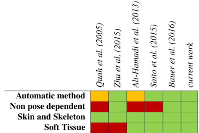
3D model editing. Tab. 1 compares state of the art anatomy 82
registration methods. 83 84 Quah et al. (2005) Zhu et al. (2015) Ali-Hamadi et al. (2013) Saito et al. (2015) Bauer et al. (2016) curr ent work Automatic method Non pose dependent Skin and Skeleton Soft Tissue
Table 1. Comparison between state of the art anatomy registration meth-ods. Legend: green means that the characteristic is totally handled by the method, orange that it is partly, and red that it is not.
User Tracking In Pfister et al. (2014), the authors assess that 85
the rough Kinect body tracking data are enough for basic mo- 86
tion measurements such as gait analysis, or joint angles during 87
motion, but are far beyond VICON cameras in terms of soft- 88
ware and hardware. 89
The tracking algorithm used in this paper is based on the 90
Kinectbody tracking skeleton which is really noisy. Whereas 91
we add constraints to upgrade the tracking, Meng et al. (2013) 92
ask the user to pinpoint anatomical key points to help position- 93
ing the data. Shen et al. (2012) use an example-based method 94
tracking is a critical step, other methods like those introduced
1
by Zhou et al. (2014) or Wei et al. (2012) use the Kinect depth
2
map and implement their own posture registration process using
3
probabilities or pose estimations. Zhu et al. (2015) use
multi-4
Kinectdepth maps and anatomical knowledge to enhance
real-5
istic limb motions.
6
Nowadays, in the game industry, sports and fitness training
7
applications based on depth map tracking devices are
com-8
monly used (e.g. Nike Kinect+, Get Fit With Mel B, Your
9
Shape, etc...). To our knowledge, the best tracking games
10
are based on the Microsoft V2.0 Kinect technology. All these
11
games only show the user depth map or silhouette .
12
By presenting the anatomy superimposed onto the user’s
13
color map (AR), a precision and a realism constraint are added
14
compared to this field state of the art. Associated Supplemental
15
materials presents experiments we did to determine the overall
16
Kinectbody tracking precision and quality.
17 18
AR Systems In the last few years, the number of AR
appli-19
cations increased in the medical education field (see Kamphuis
20
et al. (2014)).
21
The Magic Mirror, by Blum et al. (2012), superimposes
stat-22
ically CT scans of the abdomen onto the user’s image with
23
gesture-based interaction. A more recent version of the Magic
24
Mirror (see also Ma et al. (2016)) also presents an “organ
explo-25
sion effect” and the possibility to visualize precomputed muscle
26
simulation of the user’s arm in real-time. The Digital Mirror, by
27
Maitre (2014), shows full body CT scans but does not
superim-28
pose them on the user image. In these two cases, data follow
29
the user’s motion but are not deformed with respect to these
30
motions. The Anatomical Mirror, by Borner and Kirsch (2015),
31
allows full-body motion by using the Kinect body tracking, but
32
displays animated generic 3D models while we show a
user-33
specific one.
34
Thanks to the use of rules coming from anatomical
knowl-35
edge, we significantly improve AR realism and anatomy motion
36
plausibility with respect to Bauer et al. (2014) and Bauer et al.
37
(2015) in the Living Book of Anatomy project. Tab. 2
sum-38
marizes comparisons between state-of-the-art demos and our
39
work.
40 41
Data Validation Validation of anatomical data requires
in-42
vivo measurements, the simplest way is to use as ground truth
43
body measurements (see Dao et al. (2014)) or/and anatomical
44
landmarks (see Espitia-Contreras et al. (2014)) taken directly
45
onto the user’s body. The study made by Malinowski and
Matsi-46
nos (2015) gives limb bones length during motion and compare
47
them with ground truth body measurements.
48
Using user body anatomical landmarks introduces
measure-49
ment errors due to body position and skin curvature. We
de-50
cided to use MRI data as ground truth to be able to obtain
in-51
ternal specific points (e.g. femoral head of bone) in addition to
52
externally visible specific anatomical points.
53
2. User-Specific Anatomy
54
We present a novel approach using Kinect SDK outputs
55
(color map, body tracking skeleton and point cloud) and a 3D
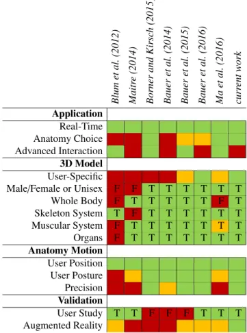
56 Blum et al. (2012) Maitr e (2014) Borner and Kir sc h (2015) Bauer et al. (2014) Bauer et al. (2015) Bauer et al. (2016) Ma et al. (2016) curr ent work Application Real-Time Anatomy Choice Advanced Interaction 3D Model User-Specific
Male/Female or Unisex F F T T T T T T Whole Body F T T T T T F T Skeleton System T F T T T T T T Muscular System F T T T T T T T Organs F T T T T T T T Anatomy Motion User Position User Posture Precision Validation User Study T T F F F T T T Augmented Reality
Table 2. Comparison between anatomical mirror-like applications. Leg-end: green for good (or True), orange for average, red for bad (or False).
reference model including skin surface and internal anatomy 57
(skeleton, muscles, organs, etc) to generate user-specific 58
anatomical data. 59
60
The method consists of four steps. First, the user-specific 61
body segment lengths and widths are computed using the Kinect 62
SDK outputs (see Section 2.1) to define a list of 3D key points. 63
In the second step the generic skin is deformed based on key 64
points and the partial user’s point cloud (Section 2.2). The third 65
step consists in transferring the reference skeleton inside the 66
user-specific skin (Section 2.3). Finally soft tissue between the 67
bones and the skin is determined using Laplacian interpolation 68
in a way similar to Ali-Hamadi et al. (2013). These different 69
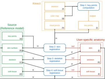
steps are summarized in Fig. 1. 70
To ease the understanding of the rest of this Section, descrip- 71
tions of each type of deformation skeleton used are provided 72
below: 73
• Kinect body tracking skeleton: composed of 25 joints, 74
this animation skeleton is given by the Kinect SDK. 75
• skin registration skeleton: composed of 22 control 76
frames and 18 control points. Control frames (Fig. 4, red 77
dots) are defined on the generic 3D skin and they corre- 78
sponds to some of the Kinect body tracking joints. Control 79
points are defined on the generic 3D skin contour (Fig. 4, 80
skin surface (b) skeleton (c) soft tissue (d) key points (a) Step 2: skin registration skin (j) Step 3: skeleton registration
Step 4: soft tissue registration skeleton (k) soft tissue (l) User-specific anatomy Kinect Source (Reference model) in in in in out out out key points (i) cloud points (h) color map (g) skeleton (f)
Step 1: key points computation
output
in in
Fig. 1. Pipeline of the user-specific anatomy generation.
computed in Section 2.2. This system is used for skin
reg-1
istration.
2
• Internal anatomy registration skeleton: composed of 96
3
joint constraints between bones and 373 control frame
po-4
sitions (see Fig. 7). This system is used to keep anatomical
5
consistency during internal skeleton registration and is
de-6
fined based on anatomical rules presented in Section 2.3.
7
2.1. Body size
8
The Kinect SDK provides a simple body tracking skeleton,
9
without temporal coherence: links may have different lengths
10
at each frame. At calibration time: starting from a T-pose
11
(Fig. 2.a), the user flexes his or her elbows (Fig. 2.b) and knees
12
(Fig. 2.c). This allows us to estimate the length of upper and
13
lower limb segments.
Fig. 2. Calibration process: (a) to have global proportions (head and torso), (b) for real upper limb parts lengths, (c) for real lower limb parts lengths. 14
15
The user silhouette and the body tracking skeleton given by
16
Kinectare needed to compute body measurements (see Fig. 3.b)
17
and define the 18 key points used for skin registration, as
pre-18
sented in Section 2.2. The Kinect body tracking skeleton is
19
mapped from camera space to image space using Kinect SDK
20
tools.
21
A key point corresponds to the intersection between the
22
user’s silhouette edge pixel and a perpendicular line computed
23
using a Bresenham algorithm. For robustness, we have
de-24
signed a silhouette detection criterion: an edge pixel is defined
25
by a black pixel followed by three white pixels to avoid silhou- 26
ette holes. 27
For each key point, the Bresenham algorithm is initialized 28
using the middle of links as starting point and the perpendicular 29
vector as the direction to follow. For instance using the point 30
in-between the shoulder and elbow link gives us the upper arm 31
width. 32
The 2D key points are mapped from image space to camera 33
space using Kinect SDK tools, Fig. 3.c shows the key points 34
we use.
Fig. 3. (a): skeleton key points. (b): body measurements key points. (c): 3D key points used in skin registration.
35 36
Due to clothing and occlusion, some dimensions might be 37
unreliable, especially thigh widths. Firstly, by assuming the 38
human body symmetric along the sagittal plane, small errors 39
in limb lengths are avoided. For each limb the average length 40
value is used as real length in both sides. Other key point posi- 41
tions are inferred based on the user silhouette and basic anatom- 42
ical knowledge. Based on an average human body, we defined 43
ratios between body parts. For instance, knowing that the thigh 44
measurement should be half of the hip measurement, the thigh 45
width can be inferred. Some validations are shown in Section 4. 46
2.2. Skin registration 47
The skin registration method is based on the silhouette key 48
points computed in Section 2.1 and the Kinect point cloud. The 49
main difficulties are the inaccuracy of the Kinect output data 50
and the fact that people clothes are captured within the Kinect 51
point cloud. To solve these issues, a new elastic deformer is 52
introduced. 53
The skin is rigged using frame-based elastic deformers 54
(Gilles et al. (2011)) corresponding to the Kinect body track- 55
ing skeleton joints (red dots in Fig. 4). Each skin vertex is 56
controlled by several frames, using linear blend skinning. The 57
skinning weights are computed using Voronoi shape functions 58
as in Faure et al. (2011). The silhouette key points (green dots 59
in Fig. 4) are mapped onto the skin to optimize the final result. 60
Instead of using global affine transformations (12DOFs) as 61
in Ali-Hamadi et al. (2013); we use 9DOFs scalable rigids as 62
frames, each bone matrix combines 3 translation, 3 rotation and 63
3 scale parameters. The advantage over affine control frames is 64
obtaining a better non-uniform local scaling to avoid shearing 65
Fig. 4. Skin registration. Red dots: origins of control frames; green dots: silhouette key points; blue dots: Kinect point cloud.
The skin model is registered to the target by minimizing a
1
weighted sum of three energies (see Gilles et al. (2011, 2013))
2
using an implicit solver.
3
The predominant energy Eskeleton = P22i=1 1 2Kd
2
i (where K is
4
the stiffness and d the distance to rest) defined by point to point
5
zero length springs, attracts the control frames of the template to
6
the bones of the user-specific model (red points in Fig. 4). Then
7
the energy Ekeypoint= P18i=1 1 2Kd
2
i, also defined by point to point
8
zero length springs, attracts the silhouette points (green points
9
in Fig. 4). Minimizing these first two energies scales the limbs,
10
the torso, the neck and the head of the generic model
accord-11
ing to the target body measurements as illustrated in Fig. 5.a
12
and b. The energy Ecloud pointattracts the skin to the target point
13
cloud using an ICP approach minimizing the distance between
14
two sets of points. At each iteration, the point to point
corre-15
spondence is reevaluated and the quadratic energy (as Eskeleton
16
and Ekeypoint) attracts each skin point to the closest target point.
17
The forces are propagated from the skin vertices to the skeleton
18
control frames (see Fig. 4 and Fig. 5.c). Thanks to the fact that
19
a small set of control frames are used, awkward configurations
20
are avoided and no smoothness or kinematic constraint terms
21
are needed.
Fig. 5. Skin registration result at the end of each step of the optimization process. (a): minimizing Eskeleton. (b): minimizing Eskeletonand Ekeypoint. (c): minimizing the three energies.
22
Fig. 6presents the skin results after registration with the
cor-23
responding Kinect point cloud. By using Ecloud point, the torso 24
skin is slightly deformed to refine the model in the same way, 25
the user being a woman or a man. 26
Fig. 6. Kinect point cloud and corresponding registered skin. Top: 1.55m female. Bottom: 1.85m male.
2.3. Internal Anatomy Registration 27
User-specific anatomy reconstruction is divided in two sub- 28
parts: anatomical skeleton registration and soft tissue registra- 29
tion. Tissues are deformed as described in Ali-Hamadi et al. 30
(2013); here the only focus is on internal skeleton registration. 31
Inputs are the 3D reference of the skin and skeleton models and 32
the estimate of the user skin registered obtained in Section 2.2. 33
First, our method uses a volumetric interpolation to estimate 34
the user anatomical skeleton. As in Ali-Hamadi et al. (2013), 35
the use of Laplacian interpolation (Fig. 8.a) with as boundary 36
condition the transformations between the two skins ensures 37
that all the internal anatomy is bounded inside the user’s skin 38
after transfer. 39
A major limitation of the Anatomy Transfer (Ali-Hamadi 40
et al. (2013)) is the fact that the joint structure of the generic 41
model is not maintained. Nothing prevents a bone from pass- 42
ing through another one (Fig. 8.b) or from being disconnected 43
from a bone to which it should be connected (for instance ribs 44
and thoracic vertebra, or ulna and humerus around the elbow 45
joint, see Fig. 8.c). To keep correct joint structures and avoid 46
these shortcomings, joint constraints between the elements of 47
our elastic bone model are added. The joint location, kinemat- 48
ics and limits are set according to Nordin and Frankel (2001) 49
(see Fig. 7). 50
Thus, the internal anatomy registration skeleton is defined 51
using frame based elastic deformations (defined in Gilles et al. 52
(2010)) with weights computed using a Voronoi shape function 53
as in Faure et al. (2011) to smoothly propagate along the bone 54
each control frame transformation. 9DOFs scalable rigids for 55
the control are used to keep head bone consistency as it is in the 56
Fig. 7. Right arm internal anatomy registration skeleton. Blue dots for control frame positions; yellow lines and middle bone frames for alignment constraints; other frames for joint constraints.
translate, rotate and scale, and thus they keep a similar type of
1
shape as in the generic bone model.
2
The list of anatomical rules used to define the internal anatomy
3
registration skeleton follows:
4
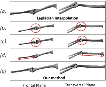
• R01: Keep long bones straightness (no bending or
twist-5
ing)
6
• R02: Keep 3D model consistency: the complete set of
en-7
tities is transferred to avoid holes
8
• R03: Keep bone head consistency
9
• R04: Keep consistency of rib cage and limbs: symmetry
10
with respect to the sagittal plane
11
• R05: Keep body joints consistency: type of joint and
12 movement amplitude 13 Transversal Plane Frontal Plane Laplacian Interpolation
(b)
(c)
(d)
Our method(a)
(e)
Fig. 8. (a): Laplacian Interpolation, (b): registration without joint con-straint (overlaps between bones), (c): registration without joint concon-straint (bone heads disconnection), (d): registration without alignment constraint (bent and twisted bones), (e): our method.
To avoid bending bones (Fig. 8.d), an alignment constraint is
14
added between the two bone heads. This constraint restrains the
15
possible displacements between the control frames in only one
16
direction defined by the line between them (see yellow lines in
17
Fig. 7). Thereby, the control frames can translate in one direc- 18
tion, but can still scale in all three directions. This alignment 19
constraint is applied to long bones only. 20
It has been shown in Zhu et al. (2015) and similar approaches 21
has been explored in Saito et al. (2015) that non-uniform scaling 22
can be used to get more plausible bone deformations. This is 23
why we introduced more control frames per anatomical bone. 24
The number of frames varies according to bone type, the goal 25
being to give enough deformability to each (for the registration 26
process) while keeping good computation times (see blue dots 27
in Fig. 7). For the short bones such as carpal bones, one frame 28
per bone is used. For the long bones such as the femur two 29
frames per bone are needed: one at the center of each bone 30
head. For the flat bones such as the ribs three frames per bone 31
are defined to keep ribs close to the skin in terms of curvature: 32
two on bone heads (e.g. close to the joints rib-vertebra and 33
rib-sternum), and one between the two others (middle of the 34
rib). For bones with more complex shape such as vertebrae 35
three frames per bone allows enough deformability to register 36
the model while avoiding overlaps (e.g. overlaps between facet 37
joints, and spinous process of two different vertebrae). 38
3. User Tracking 39
A single Kinect is used to perform body tracking. To re- 40
duce tracking noise, we record Kinect data in daylight, Kinect 41
gives better results with background and ground matte materi- 42
als. We observed that if the user’s ground reflection is too vis- 43
ible, the Kinect includes it as part of the user silhouette which 44
leads to lower limb length errors. The Kinect position is 60cm 45
off ground for good lower-limb tracking results as determined 46
in Pfister et al. (2014). 47
Because Kinect segments the depth map to compute body 48
tracking joints at each frame, link distances change from frame 49
to frame. This may lead to a disconnected anatomical skeleton 50
(on the limbs) or elongated meshes (on the torso zone). We 51
present the pipeline of our enhanced body tracking system in 52
Fig. 9. 53
Body tracking skeleton (25 joints positions)
Smoothing of small tracking noise
(Kalman filter on positions)
Realistic body tracking
(body joints position and orientations) Hierarchical body tracking system
(in-between joint distances)
Anatomically contrained joint Orientations
(dofs and angle limits)
Input :
Output :
Fig. 9. Enhanced body tracking pipeline.
Firstly we define a hierarchical body tracking system by
con-1
straining the limb lengths and by recomputing joint orientations
2
(see Section 3.1 for more details).
3
To smooth out small tracking noise, we then apply a Kalman
4
filter onto the joint positions. Joint orientations are
recom-5
puted from the filtered joint positions. Finally, we anatomically
6
constrain the joint orientations: more details are given in
Sec-7
tion 3.2.
8
3.1. Hierarchical body tracking system
9
Our hierarchical body tracking system is composed of 25
10
joints according to the Kinect SDK body tracking system.
11
To define each joint f , the position and the orientation of its
12
parent p is required. To overcome this, we begin by
comput-13
ing the joints from the root (spine base joint) to the leaves (e.g.
14
hand tips, foot joints and head joint). The root joint is defined
15
by keeping the filtered Kinect position and orientation.
(a) (b) (c) p(t0) p(t) p(t) f(t0) f(t) f(t) c(t0) c(t) c(t) R fc(t0) fc(t)
Fig. 10. (a): our hierarchical body tracking skeleton at (t0). (b): Kinect body tracking skeleton at (t). (c): our result.
16
At initialization time t0 (see Fig. 10.a), each joint position
17
is defined by our generic anatomical model and link distances
18
computed after calibration (see Section 2); and each joint
orien-19
tation is defined by the initial Kinect orientation determined in
20
KinectSDK.
21
The advantage of using a hierarchical skeleton is to obtain
22
the body pose at each time t using only the joint rotations. We
23
use the current Kinect body tracking skeleton to retrieve these
24
rotations.
25
Most often, orientations given by Kinect are incorrect so we
26
decided to recompute them using link directions by finding the
27
smallest rotation R between initial direction ( f c(t0)) and current
28
direction ( f c(t)), see Fig. 10.b. Fig. 10.c shows our hierarchical
29
body skeleton system at step t.
30
3.2. Anatomically constrained joint orientations
31
To correct non-anatomically plausible behaviors due to
track-32
ing errors, each Kinect hierarchical body tracking joint
orienta-33
tion is constrained by limiting the number of possible rotations
34
based on anatomical motion knowledge (e.g. knee joint can be
35
approximated as a 1DOF joint, whereas the hip joint is a 3DOFs
36
joint). This is done by constraining a given quaternion using
37
Euler-angle constraints to find the closest rotation matrix
de-38
fined only with valid axis within the joint limits. Computation
39
is made using the Geometric Tools library by Eberly (2008). 40
Fig. 11.aillustrates in red a raw Kinect tracking and in gray the 41
result after applying this constraint. To add even more anatom- 42
ical plausibility to the result, joint limits are added to each rota- 43
tion axis. Fig. 11.b highlights this constraint by showing Kinect 44
raw data in red and realistic angular limits obtained in gray. 45
Fig. 11. Kinect data in red and corrected in gray. (a): off angular limits rotation. (b): rotation axis error (DOFs).
4. Results and Validation 46
To our knowledge, dealing with realistic anatomy visualiza- 47
tion and motion is one of the most complex AR system ever be- 48
cause superimposing 3D anatomical data onto the user’s color 49
map reveals all the user measurement and tracking errors. 50
Our calibration method is a little time consuming (1-2sec 51
for skin registration, 15-30sec for skeleton registration and 30- 52
60sec for soft tissue registration) but allows us to obtain a 3D 53
model with accurate user measurements; moreover the motion 54
capture pipeline, even with the introduction of delay during 55
quick motions, leads to realistic and stable user tracking. 56
Thanks to these two features, the presented method allows a 57
realistic experience for understanding anatomy. The described 58
method is implemented in C++ and runs on a commodity laptop 59
(Intel CoreI7 processor at 3 GHz, Nvidia Quadro K2100M and 60
8GB of RAM). The real-time AR visualization runs between 61
35 to 62 fps depending on the 3D feedback: full-body muscu- 62
loskeletal system (49211 vertices, 95189 faces) will run at 35 63
fps whereas internal organs (20144 vertices, 39491 faces) will 64
run at 62 fps. 65
The computational bottleneck of our system is the quality 66
of the 3D model (number of faces and vertices) alongside the 67
quality of the user color map (Kinect gives a high definition 68
color map, which is reloaded at each frame). 69
We provide the visual feedback on a commodity laptop 70
screen and onto a 1.50m/2.0m screen for a demo display (see 71
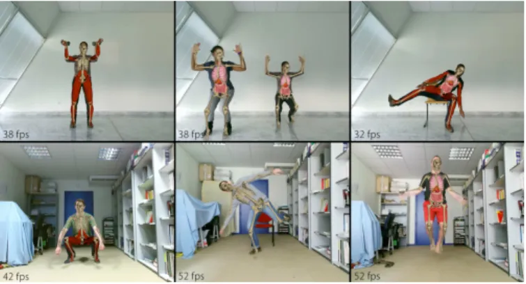
right side of Fig. 12). 72
Fig. 12presents snapshots of the provided visualization. In a 73
first set of experiments, the motion sequences were acquired for 74
4 men with an average height of 1.70m, and 3 women with an 75
average height of 1.60m. To get uniform results we work with 76
Kinectsequences made in similar environment conditions (day- 77
light, background material reflections, Kinect position, etc...). 78
Fig. 13 presents two tracking data of the same user wear- 79
Fig. 12. Left: system set-up. Right: snapshots of results.
seen on the right side that the registered skeleton for these
1
two datasets are almost identical; the red one is slightly
big-2
ger (1.2% for the limbs lengths and 2.5% for torso widths) than
3
the other one (green). This comparison allows the validation of
4
our skin registration process (see Section 2.2).
5
Fig. 13. For the same user with different clothing and hair style (Left), we obtain almost identical results (Right).
4.1. Validation with MRI
6
The major contribution of our work, and also the most
crit-7
ical point is the closeness between the user-specific anatomy
8
generated and the user’s own. As explained in Section 1, using
9
MRI data as ground truth allows us to obtain external as well as
10
internal specific anatomical points for validation purpose.
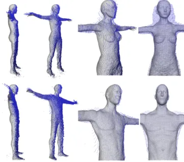
11
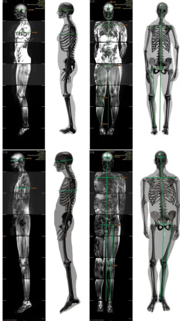
Fig. 14presents MRI data of two users (1.55m female and
12
1.85m male) in front and lateral views side to side with the
cor-13
responding 3D user-specific registered anatomies. The internal
14
anatomy registration skeleton introduced in Section 2.3 is used
15
to set the 3D model in a pose similar to MRI acquisitions.
Af-16
ter comparing body height, we found an average error of 1.5%
17
between 3D and MRI data, 3D data being always smaller than
18
MRI data. This quite small error is mainly due to limited skull
19
deformations.
20
Fig. 14. Morphometric measurements (green lines) used to compare our results with ground truth MRI data. Top: 1.55m female. Bottom: 1.85m male.
In the Kinect body tracking skeleton data, we observe a lot of 21
change in limbs lengths. Thus, we pinpoint anatomical specific 22
points (long bones protuberances) onto the MRI and onto the 23
user-specific associated 3D model. With these specific points, 24
we compare ulna and tibia lengths in real and 3D data. We 25
suffer an average 5.2% error in limb lengths : most often the 26
user-specific 3D model lacks a few centimeters. This percent- 27
age seems quite acceptable taking into account Kinect raw data 28
noisiness. 29
To evaluate the torso body part realism, we propose to com- 30
pare the user-specific 3D model and full-body MRI data by 31
comparing the distance between left and right humerus bone 32
heads. The average error between 3D and MRI data is rather 33
small: 1.5%. 34
Fig. 6 shows that the point cloud and skin are fairly close; 35
what about internal anatomy? We know that women hips are
1
in average larger than men to allow birth. The 3.1% error
be-2
tween MRI and 3D data (the 3D data being always bigger than
3
the MRI data) demonstrates that the distances between left and
4
right femoral bones head difference between women and men
5
is well transcribed in internal anatomy.
6
Using the lateral view, we pinpointed specific points to find
7
rib cage depth. The user-specific rib cage is always bigger than
8
the MRI data (around 20% bigger). It may be due to the
dif-9
ference in posture during acquisition : for MRI data, the user is
10
lying whereas for Kinect data the user is standing. It may also
11
come from the use of a partial point cloud instead of a complete
12
one. Due to front view capture, we observe depth errors in the
13
skull as well: the skull is about 12% bigger in depth in 3D than
14
in MRI data.
15
4.2. Validation with User Study
16
In a second set of experiments 20 different subjects with
17
no motor problems and working everyday on tools involving
18
medicine or medical imaging were involved. For each subject,
19
we captured a range of full body motions involving upper and
20
lower limb motion as well as torso motion. Fig. 15 presents
21
snapshots obtained during the user study.
22 23
Fig. 15. snapshots of our system obtained during the user study.
The group is composed of 13 men between 24 and 54 years
24
old (average height: 181cm, average weight: 82.6kg), and 7
25
women between 22 and 44 years old (average height: 164cm,
26
average weight: 61.7kg). This user study was designed to
27
evaluate the believability of our system. The 4-page user
28
study is composed of yes/no questions (with text space for
29
elaboration if no is the answer), augmented reality screenshot
30
comparison and correctness evaluation, rating-based questions
31
(1 to 5), and opened questions (for global feedback). Below
32
we present eight criteria extracted from the user study results,
33
which evaluation is given in Tab. 3.
34 35
Body position range (criterion C01) corresponds to motions
36
while standing, crouching or sitting. In most cases, the results
37
are well received. For other cases, limitations are directly
con-38
nected to Kinect occlusion limitations (for more information
39
cf. Associated supplemental materials).
40 41
Body orientation range (criterion C02) corresponds to 42
body orientation from Kinect point of view: e.g. facing, profile, 43
3/4, back. When Kinect raw data are occluded or self-occluded, 44
our system returns incorrect motion poses: the more occlusion 45
in Kinect raw data, the more errors we will have (for more 46
information cf. Associated supplemental materials). A major 47
topic is to be able to handle important occlusion zones, this 48
motivates the work presented in Section 5. 49 50
Motion range (criterion C03) defines simple motions like 51
flexion/extension of the knee, as well as complex motions in 52
the extremities like finger motion or supination/pronation of 53
the arm. We obtain high motion quality for simple motions; 54
for complex motions we are limited by Kinect: this criterion 55
suggest further improvements. The Kinect SDK outputs a small 56
number of joints which limits the body motion possibilities 57
(e.g. spine bending). 58
59
For Motion fluidity and delay (criterion C04) and Motion 60
consistency (criterion C05), the goal is reached. Motion 61
consistency refers to the absence of outliers during motion. We 62
should state the fact that part of the visual latency that might 63
occur comes from the low frame rate of the color map display. 64 65
Motion plausibility (criterion C06) corresponds to joint 66
DOFs and angular limits. For this criterion we obtain different 67
results depending on the body segment studied. For instance, 68
it is easier to implement constraint for 1DOF joints than for 69
3DOFs joints such as spine or shoulders joints due to motion 70
range. Work presented in Section 5 allows us to obtain better 71
results on this criterion. 72 73
Anatomy realism (criterion C07) gives a feedback on the 74
registration method by focusing on limb length and torso 75
width. For this criterion, people with professional knowledge 76
in anatomy were the only ones to rate the user-specific anatomy 77
as average. 78
79
For almost everyone, the Augmented reality (criterion C08) 80
results were of good level. The overall quality can even be in- 81
creased with mesh texturing, or by adding a transition effect 82
between virtual and real data (e.g. 3D anatomy and the user’s 83
color map).
C01 C02 C03 C04 C05 C06 C07 C08 −− 00% 15% 05% 00% 00% 10% 00% 00% +− 20% 50% 30% 10% 10% 25% 15% 05% ++ 80% 35% 65% 90% 90% 65% 85% 95%
Table 3. User study compiled results according to quality criteria for a mirror-like augmented reality system. For each criterion: the percentage of bad/average/good reviews.
84
5. Towards Image-based Corrective Registration 85
In Section 2 and 3 we proposed a system that can efficiently 86
register user-specific anatomy and provide interactive visual- 87
this section, we will refer to this system as the “3D registration
1
system”.
2
The feedback obtained during the user study (see Section 4.2)
3
suggests that a supplementary process for better quality of the
4
overlay is needed. Anatomy misalignments are in particular
5
visible when presenting anatomy superimposed onto the user’s
6
color map (AR). For example, anatomical limbs can sometimes
7
be out of the user’s silhouette as shown in Fig. 16 (e.g. arms
8
and hands). We avoid performing these corrections in our 3D
9
registration system as they make it overly constrained.
10
Image-based Correction In this section, we describe a
11
method to solve this problem efficiently in image domain. Our
12
image-based corrective registration allows to reduce the errors
13
that accumulate during previous system steps such as motion
14
capture, anatomy transfer, image generation and animation.
15
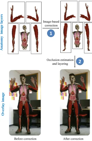
Occlusion Handling We perform these image-based
correc-16
tions for separate regions of the registered 3D anatomy (see
17
Fig. 16). To generate the final overlay image we have to
deter-18
mine in which order these corrected images should be layered.
19
Therefore, we propose an image-based occlusion handling
tech-20
nique that automatically decides how to overlay these images
21
relatively to each other in the final AR rendering.
22
5.1. Input Data From 3D Registration
23
By projecting and rendering registered 3D anatomy on the
24
2D color map we generate anatomy images (Fig. 16 top row)
25
corresponding to a set of predefined 3D anatomy regions. Each
26
anatomy region is composed of a specific set of bones, organs
27
and muscles of the registered 3D anatomical model. For
ex-28
ample, in Fig. 16, we show the anatomy images corresponding
29
to the five anatomy regions we use in our examples.
Unfor-30
tunately, after superimposing them onto the color map we can
31
clearly observe that they are misaligned (see Fig. 16
bottom-32
left). Using our image-based correction, we deform or warp
33
these anatomy images to correct the misalignments. In
Sec-34
tion 3 we defined our enhanced body tracking system
com-35
posed of 25 joints. By mapping it to image space, we
gen-36
erate Anatomy landmarks. The same is done with the Kinect
37
SDK body tracking skeleton to generate Kinect landmarks. Our
38
image-based correction method uses these two sets of
land-39
marks and the Kinect depth map to correct the anatomy
mis-40
alignments.
41
As mentioned earlier, to solve the problem of anatomy
mis-42
alignment due to accumulation of errors in the 3D registration
43
system, we propose an image-based correction method.
Cor-44
recting these errors in a reduced dimension (in image space)
45
causes small projective errors to occur, but these corrections
46
can be performed very efficiently. Furthermore, the result of
47
the 3D registration system is a 2D image that mixes the real
48
world captured by the Kinect with a simulated image of the
ani-49
mated model; therefore making the correction at the very end of
50
the process makes it possible to correct errors of all the stages
51
including the final visualization in 2D. The two main stages of
52
our algorithm are: (a) image-based correction and (b) occlusion
53
estimation and layering. The overview of this pipeline can be
54
seen in Fig. 17.
55
Fig. 16. We propose an image-based correction (step 1), and an occlusion estimation and layering technique (step 2). In the first step, we correct anatomy regions separately. In the second step, we combine them in cor-rect order to generate the final overlay image.
5.2. Image-based Correction 56
The image-based correction stage can be further divided into 57
three steps: (a) feature estimation, (b) landmark correction and 58
(c) updated anatomy image generation. 59
5.2.1. Feature Estimation 60
We estimate two types of image features: first, we find a set 61
of anatomy features S in the anatomy images, and second, a 62
set of depth features D in the Kinect depth map. Let’s con- 63
sider that we have N (=5 in our examples) anatomy regions. 64
Subsets of the Kinect and anatomy landmarks are assigned to 65
each of the anatomy regions based on the contribution of the 66
3D joints corresponding to these landmarks in producing soft 67
tissue movements in that region. We also describe below, how 68
we can estimate N depth contours corresponding to the anatomy 69
regions and estimate depth features from these regions. 70
We estimate depth contour points by first detecting edges 71
corresponding to the depth discontinuities in the Kinect depth 72
map using Canny edge detector (Canny (1986)) and then com- 73
Fig. 17. Overview of our corrective registration system.
proposed in Suzuki et al. (1985). Contour segmentation is a
1
well researched topic and more recent work, such as Hickson
2
et al. (2014); Abramov et al. (2012); Hernandez-Lopez et al.
3
(2012) can also be used. For each contour point we find the
4
closest Kinect landmark. Conversely, after that, for each Kinect
5
landmark we obtain a set of depth contour points. For an
6
anatomy region, we estimate depth contour by taking union of
7
all depth contour points corresponding to the Kinect landmarks
8
of that region. Similarly, we estimate anatomy contour of an
9
anatomy region by estimating the contour around the rendered
10
anatomy in the corresponding anatomy image.
11 12
Fig. 18. Feature estimation for left arm. In left: anatomy features (S) (blue) are estimated using anatomy landmarks (red) and sub-landmarks (green). In right: depth features (D) are estimated using Kinect depth landmarks (red) and sub-landmarks(green). Here we are showing one sub-division of landmarks.
Anatomy Feature Estimation We denote the anatomy
13
features for the ith anatomy region as Si, which are estimated
14
in the corresponding anatomy image. For each anatomy
15
landmark of the anatomy region we estimate a normal vector
16
with a direction which is average of the normals to the lines
17
connecting the landmark to the adjacent anatomy landmarks.
18
This vector intersects the anatomy contour at two points and
19
we add these points to Si. If desired, the lines can be further
20
sub-divided to generate sub-landmarks increasing the number
21
of features, in our implementation we subdivided the lines
22
6 times. Adding more features increases the robustness by
23
reducing the contribution of outliers, see Fig.18.
24 25
Depth Feature Estimation We denote depth features of the
26
ith anatomy region as Di. Similar to the estimation of anatomy 27
features, we can estimate depth features by finding intersections 28
of the normal vectors from Kinect landmarks with the depth 29
contour of the anatomy region (see Fig. 19). Depth contours 30
are mostly fragmented and not closed because the transition be- 31
tween anatomy regions generates depth discontinuities. Since 32
we have missing points in the contour, sometimes normal vec- 33
tors do not intersect with depth contours. In that case, we do not 34
add any depth features to the depth landmark. At the same time, 35
we drop anatomy features of the corresponding anatomy land- 36
mark to ensure one-to-one correspondences between anatomy 37
and depth features. Depth maps are often noisy and causes 38
erroneous depth feature estimation due to noise in the Kinect 39
depth sensor raw data. We apply a Kalman filter onto the depth 40
feature locations to remove the noise effect. 41
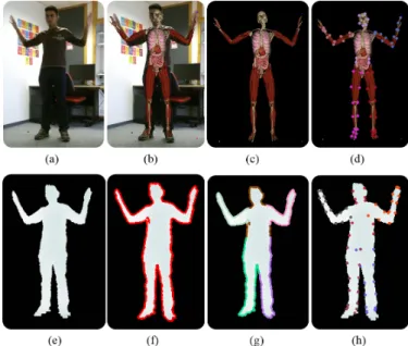
Fig. 19. Feature estimation: Preliminary 3D registration when superim-posed on input image (a) we can observe anatomy misalignments (b). We estimate anatomy features (d) from the intermediate anatomy images (c). In the bottom row, we show the estimation (f) and segmentation (g) of depth contours from the depth map (e), and estimated depth features (h).
5.2.2. Landmark Correction 42
Kinectlandmarks provide a reasonable estimate of the skele- 43
ton in the 2D image space, we will call it Kinect 2D skeleton. 44
the anatomy landmarks as anatomy 2D skeleton. But if we warp
1
our anatomy regions using a map learned from anatomy
land-2
marks to Kinect landmarks, it does not ensure that the mapped
3
regions will entirely reside within the depth contours. To
main-4
tain smoothness in shape at boundary of the warped region, we
5
look into a reliable warp map, we call T .
6
We use a thin plate spline-based interpolation (see Bookstein
7
(1989)) represented with radial basis functions (RBF) to
ap-8
proximate the mapping T from anatomy features to depth
fea-9
tures. This mapping is composed of an affine transformation
10
and a non-affine deformation. We use a regularizer parameter
11
λ to control the influence of the non-affine deformation part,
12
which refers to a physical analogy of bending. More recent
13
techniques, such as Sorkine and Alexa (2007) can also be used
14
to compute the image warp map.
15
For an anatomy region with M feature points. The parame-ters of the RBF function are estimated by solving the following Eq. 1: Di= A Si+ λ X i=1:M X j=1:M (wjR(||si− dj||)) (1)
Where, Diand Siare Mx2 matrices containing respectively
lo-16
cations of depth and anatomy features. siand diare locations
17
of ith anatomy and depth features, A is a MxM affine
trans-18
formation matrix. w represents weight of non-affine bending
19
transformation, and R(r) = r2 log(r) is a RBF function.
Addi-20
tionally, we include Kinect landmarks and anatomy landmarks
21
respectively in the matrices D and S.
22
We can rewrite Eq. 1 in matrix form as:
Di= " K(R) PT(Si) P(Si) 0 # "W A # , (2)
Where, P contains homogenized Si, K contains values of RBF
functions and W is a vector with non-affine weights. We can further simplify Eq. 2 as Di = Mi(Si) Xi, where Mi and Xi
represent the first and second matrix of the right hand side of Eq. 2. Now, by combining equations of all the body parts in one global equation, we can write:
D1 .. . DN = M1(S1) · · · 0 .. . ... ... 0 · · · MN(SN) X1 .. . XN (3)
We can rewrite Eq. 3 as:
D= ˜M(S) ˜X (4) In our current implementation N=5, size of ˜M and D are
23
240 × 240 and 240 × 2 respectively. Finally, we can also write
24
Eq. 3as D = T ( ˜M(S), ˜X. where, T maps anatomy features in
25
S to the depth features in D, and ˜Xincludes the parameters of
26
the mapping.
27
We solve Eq. 4 to estimate mapping parameters ˜X of T by
28
formulating it as a linear least squares system for given S and
29
D which includes anatomy and depth features that have
one-30
to-one correspondences. In our regularized optimization
frame-31
work, we constrain the anatomy landmarks with soft constraints
32
to map Kinect landmarks. T can be used to warp anatomy 33
regions such that they remain enclosed within the depth con- 34
tour while maintaining a smooth boundary shape. Note that 35
T is composed of N separate mappings corresponding to the 36
anatomy regions. By remapping the anatomy landmarks using 37
T , we also obtain a better estimate of the original Kinect 2D 38
skeleton formed by Kinect landmarks, which we call updated 39
2D skeleton. Furthermore, to ensure the connectivity of land- 40
marks across different anatomy regions, we set the location of 41
shared landmarks to the average of their estimates for different 42
anatomy regions. Fig. 20 shows the resulting landmark correc- 43
tions. 44
Fig. 20. Landmark correction: Our skeleton correction algorithm corrects initial Kinect 2D skeleton in image space (b) to produce more consistent configurations (c).
Note that depth contours are noisy if the user wears loose 45
clothes, which in turn makes the depth features noisy. There- 46
fore, we prefer to maintain a smooth shape of the mapped 47
anatomy region instead of mapping anatomy features exactly to 48
the depth features. By picking a suitable λ in Eq. 1 we can con- 49
trol the smoothness. In our current implementation we chose 50
λ = 0.01. 51
5.2.3. Updated Anatomy Image Generation 52
As explained previously, to each anatomy region corre- 53
sponds an anatomy image, therefore, to warp an anatomy 54
region, we simply need to warp the corresponding anatomy 55
image. We decided to separately warp each of these images 56
based on the transformation from anatomy 2D skeleton to 57
updated 2D skeleton. To obtain the final anatomy corrected 58
rendered image, we combine these warped anatomy images to 59
a single composite image. For each pixel of that composite 60
image, we should render the anatomy region closest to the 61
camera (e.g. smallest depth value). To estimate the closest 62
anatomy region, we propose a novel occlusion estimation and 63
layering algorithm. 64
65
Image Warping We generate bounding boxes, which we call 66
anatomy cages, around links of the updated 2D skeleton. Now, 67
our goal is to deform these anatomy cages based on the defor- 68
mation field. Fig. 21 shows warping of the right upper limb 69
with cages. 70
Using T as a deformation field is not a good choice for two 71
Fig. 21. Cage generation and warping of the right upper limb. Yellow points are anatomy landmarks, White ones are updated landmarks. The red zones present anatomy cages.
we introduced in the post-processing step (where we modify
1
the locations of mapped anatomy landmarks). Second, T is
re-2
liable within the regions enclosed by the anatomy landmarks,
3
but if we use these landmarks to generate the cages, we will
4
end up having a piecewise linear approximation of the
bound-5
ary of the anatomy in the image space. Therefore, we chose
6
to use wider cages to get a smoother anatomy boundary after
7
warping. This puts the cage points outside the regions enclosed
8
by the landmarks and so we cannot use T reliably. Therefore,
9
instead of T , we use dual-quaternion skinning (Kavan et al.
10
(2008)) driven by the skeleton to perform image warping from
11
anatomy to updated 2D skeleton landmarks. Using this, we
es-12
timate deformed anatomy cages corresponding to each of the
13
anatomy cages. To warp the anatomy images, we triangulate the
14
anatomy cages, and then we estimate affine transformation of
15
the individual element of the cages from original anatomy cage
16
to the deformed anatomy cage configuration. Using bilinear
in-17
terpolation we then warp the anatomy image pixels inside the
18
triangles. We call the new warped images as warped anatomy
19
images. We define one for each anatomy region. Fig. 22 shows
20
warping results for the complete set of anatomy images.
21
5.3. Occlusion Estimation and Layering
22
As mentioned before, the main challenge in generating final
23
composite imageof the warped anatomy images is to figure out
24
which anatomy region is closest to the camera for a given view.
25
If images are naively combined as layers, occlusions such as in
26
Fig. 23, (b)can occur. In this case, the anatomy region
corre-27
sponding to the torso is occluding the hands, which is not what
28
we expect. Our method described below tackles this problem.
29
We first generate synthetic depth images for the anatomy
re-30
gions based on the Kinect 2D skeleton. For each anatomy
re-31
gion, we know 3D configuration of the corresponding Kinect
32
joints in the Kinect 2D skeleton. We model cylindrical
primi-33
tives around the bones. The radius is set equal to the maximum
34
cross-section radius of the corresponding anatomy region.
Us-35
ing the projection matrix of the camera, for each anatomy
re-36
gion, we render a depth map. We call this image anatomy
37
depth image.
38
Fig. 22. Image-based corrective registration: Misalignments in the anatomy regions observed in (a) are corrected by our image-based corrective algo-rithm to produce (b).
The size of the warped anatomy images and the composite 39
image are the same. For each warped anatomy image, we cat- 40
egorize the pixels into two types: valid when pixels belong to 41
anatomy, and invalid when they do not. In the composite image 42
domain we loop through all the pixels: for each pixel, we check 43
if at that location any of the warped anatomy images contains a 44
valid pixel. If not, we set that pixel to black. If yes, we check 45
which of the warped anatomy images contain valid pixels. Out 46
of all those warped anatomy images we pick the one that is clos- 47
est to the camera. The distance from the camera is determined 48
based on anatomy depth images. We then update the pixel of the 49
composite image with the color of that closest warped anatomy 50
image. In Fig. 23 (c) we can see how our algorithm corrected 51
the problem of occlusion (b). 52
Fig. 23. Occlusion handling: Our image-based corrective algorithm cor-rects misalignments in the rendering (a) of initial 3D registration by warp-ing anatomy regions in image space and in separate layers. Renderwarp-ing them without knowing their relative distances from camera create occlu-sions (b). Our occlusion handling algorithm can recover these relative dis-tances and render these regions in correct order (c).
5.4. Evaluation
1
We have shown qualitative results of our landmark correction
2
in Fig. 20, where we used non-linear thin plate spline-based
3
interpolation to model the deformation. Fig. 22 shows how
4
we improve anatomy registration by applying dual-quaternion
5
skinning based on deformations produced by landmark
correc-6
tion. The results of our occlusion handling algorithm is shown
7
in Fig. 23. We quantitatively analyze the results of our
image-8
based corrective registration using an anatomy intersection
co-9
efficient η. If nf is the total of anatomy pixels in the final
com-10
posite image and nkis the total of anatomy pixels that also
be-11
long to the user according to the Kinect depth map. We can
12
define η as: η= nk
nf. In Tab. 5.4, results are shown for two video 13
sequences and they clearly indicate the improvement after
ap-14
plying our image-based corrective registration algorithm. Our
15
unoptimized routines take around 75ms per frame to perform
16
this correction.
Video Before After Squat motion 0.939 ± 0.184 0.994 ± 0.026 Hand crossing 0.961 ± 0.159 0.988 ± 0.089
Table 4. Image-based corrective registration results: anatomy intersection coefficient before and after corrections
17
Fig. 24 shows the temporal profile of η for individual
18
anatomy regions in the squat motion video. Anatomy regions
19
are represented with different colors. As we can see, η
consis-20
tently remains close to 1 after our corrections. Thus,
image-21
based correction drastically reduced the alignment errors.
22
Furthermore, we can make our corrective registration faster
23
by generating warped anatomy images only when the η value
24
of an anatomy region is below a certain threshold (which means
25
they are not well aligned). For example, in the 81 frames of the
26
squat motion video we originally estimate 405 warped anatomy
27
images (e.g. 81 (number of video frames) × 5 (number of
28
anatomy regions)). If we set the threshold of η to be 0.9, we
29
reduce this number to 137: this is a 66.2% reduction.
30
Fig. 24. The anatomy alignment coefficients for anatomy regions are shown before and after image-based correction for the squat sequence.
In the 3D registration system, the errors in orientation of the
31
anatomy regions produce wrong color maps of the anatomy
re-32
gions. Since we use these color maps as color or texture of
33
the anatomy regions, we cannot correct orientation errors in the
34
image-based correction step. Currently, integration of the pro- 35
posed image-based corrective registration step within the 3D 36
registration system is not real-time. The image-based correction 37
uses color maps rendered by the 3D registration system. In our 38
current implementation, we save these color maps to the disk 39
and read them later for image-based corrections. These com- 40
putationally expensive file operations prevent real-time image- 41
based misalignment correction. Furthermore, with the current 42
latency, the combined system does not satisfy “motion fluidity 43
and delay”(criterion C04 as mentioned in Section 4.2). 44
6. Conclusion 45
We present the first live system of personalized anatomy in 46
motion. Superimposing the anatomy onto the user’s image 47
allows us to create a real-time augmented reality experience. 48
The first paper version Bauer et al. (2016) attached video (see 49
https://youtu.be/Ip17-Vaqqos) illustrates the application pipeline 50
and shows AR results of our system (before image-based cor- 51
rective registration presented in Section 5). 52
We also proposed an image-based corrective registration to 53
correct the errors that build up during system steps: motion cap- 54
ture, anatomy transfer, image generation and animation. Cur- 55
rently, the combined pipeline is not real-time due to expen- 56
sive file read and write operations. Using unoptimized code 57
for image-based corrective registration we currently achieve a 58
frame rate of 12fps on average for the combined pipeline. In 59
future, we plan to read color maps from memory instead, and 60
build a combined real-time system. Another limitation of the 61
current image-based correction is that we cannot correct the er- 62
rors in orientation of the anatomy regions relative to the bones. 63
In future, to solve this problem, we can use an image-based 64
hybrid solution, such as Zhou et al. (2010); Jain et al. (2010); 65
Richter et al. (2012) that use a 3D morphable model to fit to 66
some features in 2D images. In our case, we can model our 3D 67
anatomical reference model as a morphable model and then fit 68
it based on 2D joint locations of the updated Kinect 2D skele- 69
ton. Then, we can re-render the anatomy regions from camera 70
view to generate updated anatomy images. This should be able 71
to recover the color of anatomy regions that get occluded due 72
to orientation error in 3D registration system. After that we can 73
follow our usual skinning and occlusion handling routines to 74
generate final results. We believe that the basic Kinect body 75
tracking enhanced with our method is sufficiently accurate for 76
our needs. 77
The system could be extended or improved in different ways. 78
Posture reconstruction proposed by the Kinect SDK could be 79
replaced by more sophisticated approaches such as presented in 80
Liu et al. (2016). This could make the system not only more ro- 81
bust but also more independent of the selected sensor. Another 82
solution could be the use of physical priors such as introduced 83
in Andrews et al. (2016). It would certainly enable suppressing 84
some outliers resulting of Kinect data. On the other hand, the 85
addition of biomechanical simulations could allow to get more 86
realistic deformations of soft tissue and organs but this could be 87
at the cost of interactivity. 88