Comparative assessment of several SPECT scatter correction methods using SimSPECT

(1)

Comparative Assessment of Several SPECT

Scatter Correction Methods using SimSPECT

by

An Lu

Submitted to the Department of Nuclear Engineering

in partial fulfillment of the requirements for the degree of

Master of Science in Nuclear Engineering

at the

MASSACHUSETTS INSTITUTE OF TECHNOLOGY

September 1996

©

Massachusetts Institute of Technology 1996. All rights reserved.

A uthor ...

.. . ... . ...

Department of Nuclear Engineering

August 23, 1996

Certified by....

J. C. Yanch

Professor

s Supervisor

Certified b.

A. B. Dobrzeniecki

Research Scientist

Thesis Supervisor

Accepted by ...

Chairman,

/ I/ -

J. Freidberg

Departmental Committee on Graduate Students

MAY 19 1997

L1BRA f1iES

$1

e L-encC

(2)

Comparative Assessment of Several SPECT Scatter

Correction Methods using SimSPECT

by

An Lu

Submitted to the Department of Nuclear Engineering on August 23, 1996, in partial fulfillment of the

requirements for the degree of Master of Science in Nuclear Engineering

Abstract

Scattered photons carry misplaced positional information about the source distribu-tion, resulting in lower image contrast and inaccurate quantitation in SPECT im-ages. Correction for scatter will improve image contrast for better image quality and quantification. This thesis project implements a MCNP-based SPECT simulation system, SimSPECT, to investigate the performance of nine scatter correction meth-ods which are divided into two categories: five energy window methmeth-ods, including the dual-energy window method (DEW), the dual-photopeak window method (DPW), the channel ratio method (CRM), the three-window method using trapezoidal ap-proximation, and the three-window method using triangular approximation; and four spatial analysis methods, including the Axelsson LSF convolution method, the Floyd LSF deconvolution method, the 2D PSF deconvolution method, and the 3D PSF deconvolution method. A cold-spot hot-background phantom and a resolution phan-tom are simulated to generate projection images for scatter correction. None of the methods is found to have strictly valid assumptions. A comparative assessment of these nine scatter correction methods is made based on image contrast improvement, image mottle level, image resolution improvement and ease of implementation. Re-sults show all of the scatter correction methods lead to 5% - 25% improvement in the image contrast of the largest three cold spots in the cold-spot hot-background phantom and some improvement in the resolution of the resolution phantom. There exists a compromise between the contrast improvement and the image mottle level. None of the nine methods can perform best for all four criteria.

Thesis Supervisor: J. C. Yanch Title: Professor

Thesis Supervisor: A. B. Dobrzeniecki Title: Research Scientist

(3)

Acknowledgments

Most especially I would like to thank Professor Jacquelyn Yanch for her wise direction and tactful advice. I would also like to thank Dr. Andy Dobrzeneichi for his initial guidence in SimSPECT, and many useful discussions in the SPECT area.

Also I am very grateful to Marie-Jose Belanger for her constant help during various parts of this project. Thanks to Edward Baik, Haijun Song, Dr. Ainat Rogel and William Howard for their support and encouragement.

(4)

List of Figures

1-1 The basic components of a conventional imaging system. . ... 12 1-2 The interactions of emitted photons with the object and collimator. . 14

2-1 Definition of the energy window settings overlaid on an energy

spec-trum of Tc99m photon source ... 19

2-2 Definition of the energy window settings of three-window methods of using trapezoidal approximation and triangular approximation... 23

3-1 The cold-spot hot-background phantom. . ... 34 3-2 The extended cylinder phantom used for validation of the old-spot

hot-background phantom. ... 35

3-3 The projection images through photopeak window and scatter window and their projection profiles ... 36 3-4 The cross-sectional image of the resolution phantom as generated using

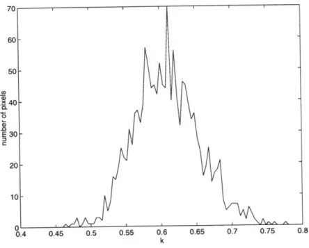
MCNP's internal plotting routine ... 37 4-1 Histogram of k within the ROI of a typical projection image. ... 44 4-2 A typical projection image (128 x 128) of the cold-spot hot-background

phantom. ... 44

4-3 Reconstructed images resulting from photopeak window acquisition (uncorrected) and DEW scatter corrections with k = 0.5 and k = 0.6062. A comparison of the measured contrast in each cold spot is shown on the upper right figure... .. 46

(8)

4-4 Reconstructed images resulting from the scatter component within the photopeak window and the scatter window ... 46 4-5 Plot of SUR(i) against R(i) in the Dual-photopeak window method

(represented by *). The result of the fitting SUR(i) = A R(i)B + C is shown as a solid line . ... ... 48 4-6 Reconstructed images resulting from uncorrected projections within

the photopeak window, and from projections scatter-corrected by the DPW method and the CRM method. Measured values of image con-trast in each cold spot are also shown. . ... 48 4-7 Histogram of G(i) and H(i) in the Channel Ratio Method ... . 50 4-8 Total scatter spectrum within the photopeak window, with the

trape-zoidal approximation and the triangular approximation. ... 52 4-9 Reconstructed images resulting from uncorrected projections within

the photopeak window, the projections scatter-corrected by three-window trapezoidal approximation and by triangular approximation. A com-parison of the contrast measured in each cold spot is also shown. . . . 54 4-10 The scatter spectrum and total (scatter + nonscatter) spectrum in

pixel (64, 64) and pixel (60, 60) of a typical projection image. In all four figures, the horizontal axis represents energy (keV) and the vertical axis represents number of photons. . ... 55 4-11 Line Spread Function and Scatter distribution function in Axelsson

M ethod . . . .. .. . 57 4-12 Axelsson-estimated scatter component compared with true scatter

com-ponent . . . .. .. . 58 4-13 Uncorrected projection slice profile compared with scatter-free

projec-tion slice profile . . . . . . . .. 59 4-14 Axelsson-corrected projection slice profile compared with scatter-free

projection slice profile ... 60

4-15 Floyd-estimated scatter component compared with true scatter com-ponent . . . .. .. . 61

(9)

4-16 Floyd-corrected projection slice profile compared with scatter-free pro-jection slice profile ... . ... . . .. . . .. . .. .. .. .. .. . . 62 4-17 Reconstructed images resulting from scatter-corrected projections

us-ing Axelsson method and Floyd method . ... . . . 63 4-18 Reconstructed images resulting from projections scatter-corrected by

2D PSF deconvolution method and 3D deconvolution method . . .. 65 4-19 Comparison of image contrast resulting from different scatter

correc-tion m ethod . . . .. . 67 4-20 Profiles of the 5-sphere group of resolution phantom using different

scatter correction methods (set 1) . ... . 71 4-21 Profiles of the 5-sphere group of resolution phantom using different

scatter correction methods (set 2) . ... . 71 4-22 Profiles of the 5-sphere group of resolution phantom using different

scatter correction methods (set 3) . ... . 72 4-23 Contrast definition for the 5-sphere profile . ... 72

(10)

List of Tables

4.1 The estimation error of the trapezoidal approximation and the tri-angular approximation of the scatter spectrum within the photopeak

window. ... .. 52

4.2 Comparison of unscatter photons at 126 and 154 keV . ... 53 4.3 Comparison of contrast and mottle produced by the 2D PSF

deconvo-lution with different y... ... 64

4.4 Image mottle and contrast resulting from different scatter correction m ethods . . . .. . 68 4.5 Contrasts of the 5-sphere profile resulted from different scatter

correc-tion m ethods . . . 73 4.6 The ease of implementation of each scatter correction method. .... 75 5.1 Summary of the comparison of nine scatter correction methods. The

performance of each method in terms of each criterion is roughly given a grade ranging from "excellent" to "poor". . ... . 78

(11)

Chapter 1 Introduction

1.1 Nuclear Medicine and SPECT

Nuclear medicine, or nuclear medical imaging, is based on detecting nuclear radiation emitted from the body after introducing a radiopharmaceutical inside the body to tag a specific physiological function [1]. The radiopharmaceutical may emit photons

in the form of X-rays or gamma rays, or alternatively, it may emit positrons (which immediately annihilate to produce two 511 keV photons). As long as the photons emanating from the radionuclide have sufficient energy to escape from the human body in significant numbers, images can be generated that portray the in vivo distri-bution of the radiopharmaceutical. Diagnostic nuclear medicine is successful for two reasons: (1) It can rely on the use of very small amounts of materials (picomolar con-centrations in chemical terms) thus usually not having any effect on the process being studied, and (2) The radionuclides being used can penetrate tissue and be detected outside of the patients without affecting organ functions. In general, nuclear medicine can be divided into three categories: conventional or planar imaging, positron emis-sion computed tomography or PET, single photon emisemis-sion computed tomography or

SPECT.

(12)

x position I

z signal pulse-height

positioning circuitry analyzer

photomultiplier tubes

scintillation crystal

I I I I I I I

I

I I

I

I I

I

I I I I I I

collim ator

Figure 1-1: The basic components of a conventional imaging system.

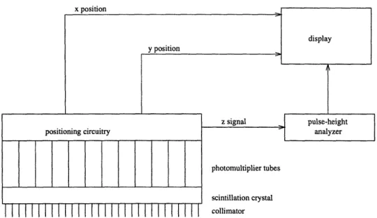
In the conventional mode, the three-dimensionally distributed radiopharmaceutical is imaged onto a planar or two-dimensional surface, producing a projection image. Conventional imaging usually employs a physical collimator attached to a large NaI (TI) crystal which is coupled to an array of photomultiplier tubes (PMT) (see Fig-ure 1-1). The purpose of the collimator is to physically confine the direction of the incident photons reaching the scintillation crystal to those directions normal to the detection plane and thereby to localize the site of the emitting sources. The basic principles of conventional imaging are as following [2]: The energy deposited by the photons reaching the detection crystal is converted into visible light photons which reach the photocathode of the PMTs where they are converted into electrons, multi-plied, and finally converted into an electrical signal at the anode of the each PMT. The amplitudes of the anode signals from each anode are then examined by analog or digital positioning circuitry to estimate the x, y coordinates of the scintillation event on the crystal. In addition, the output from each tube is summed to produce a "z signal" proportional to the total energy deposited in the crystal by the scintillation event. Pulse height discrimination is then applied to the "z signal" to retain only

display

y position

it

x position

(13)

those events where the total energy deposited in the crystal lies within a prescribed energy window. The (x,y) coordinates of each count passing the pulse height discrim-ination are stored to produce a projection image where the projection axis is normal to the plane of the collimator.

1.1.2 PET and SPECT

Conventional imaging techniques suffer from artifacts and errors due to superposition of the underlying and overlying objects that interfere with the region of interest. The techniques of computed tomography (CT) can be used to obviate the superposition problems and provide an in vivo quantitative estimate of the distribution of radio-pharmaceutical in three dimensions. Single photon emission computed tomography (SPECT) is a medical imaging modality that combines conventional nuclear medical imaging techniques and computed tomography (CT) methods [3]. The gamma pho-tons emitted from the radioactive source are detected by radiation detectors similar to those used in conventional nuclear medicine. The CT methods requires projection (or planar) image data to be acquired from different views around the patient. These projection data are subsequently reconstructed using image reconstruction methods that generate cross-sectional images of the internally distributed radiopharmaceuti-cals.

As another major emission computed tomographic (ECT) method, PET differs from SPECT in the type of the radionuclides used. PET uses radionuclides such as C-11, N-13, 0-15, and F-18 that emit positrons. When a positron is emitted and combined with a nearby electron, two annilation photons, each with an energy of 511 keV, are generated simultaneously and travel in opposite directions, nearly 180 back to back. Thus it is possible to identify the annihilation event or the existence of the positron emitters through the detection of the two photons by two detectors posed exactly in opposite sides within a short time [4].

Because of its unique coincidence detection property, PET usually can achieve higher sensitivity and resolution than SPECT [1]. However, the positron emitting radionuclides have very short half-lives, often requiring an on-site cyclotron for their

(14)

collimator

crystal

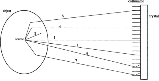
Figure 1-2: The interactions of emitting photons with the object and collimator. Photon transportation track 1, without photoelectric absorption and scatter; track 2, photoelectric absorption; track 3, blocked; track 4, scatter in object; track 5, scatter in collimator; track 6, scatter in object and then be blocked; track 7, scatter in both object and collimator.

production. Also, detection of the annihilation photons requires expensive imaging systems. SPECT uses more readily available radionuclides such as Tc99m which has a half-life of 6.02 h and is produced via decay of a long-lived (T1/2 = 66 h) parent

Mo99. Subsequently, the cost of SPECT instrumentation and of performing SPECT are substantially less than PET. Furthermore, substantial advances have been made in the development of new radiopharmaceuticals, instrumentation, and image processing and reconstruction methods for SPECT. The results are much improved quality and quantitative accuracy of SPECT imaging. These advances, combined with relatively lower costs, have made SPECT an increasingly more important diagnostic tool in nuclear medicine clinics.

1.2 Scatter problem in SPECT

The emitted photons experience interactions with the object and the collimator through basic interactions of radiation with matter (see Figure 1-2). The

(15)

photo-electric effect absorbs all the energy of the photons and stops their emergence from the patient's body or penetration through the collimator septum. The other major interaction is scattering including coherent scatter and Compton scatter. Coher-ent scatter changes the photon direction without any influence on its energy, while Compton scatter, which happens far more frequently at nuclear medicine energies than coherent scatter, not only changes the photon direction but also reduces the photon energy with a reduction dependent on the scatter angle. For the primary photons from the most common radionuclides used in SPECT, e.g., Tc99m with an emission energy of 140 keV, the probability of pair production is zero.

Photons that have been scattered before reaching the radiation detector, in the object and/or in the collimator, provide misplaced spatial information about the origin of the radioactive source. The results are inaccurate quantitative information and poor contrast in the SPECT images. Thus a scatter correction is essential, not only for better image quality and quantitative accuracy, but also for lesion detection and image segmentation. For the latter case, the accuracy of the calculated volume will be affected if the boundary of an activity region is distorted by scatter events.

While coherently scattered photons are virtually indistinguishable (on the de-tection plane) from a primary photon because of their unchanged energy, Compton scattered photons are of lower energy than the primary photons and could therefore, in theory, be completely rejected by setting the baseline of the discriminator win-dow at an energy equal to - or only slightly lower than - the energy of the primary photons. However, in a typical scintillation camera system using NaI(TI) crystals, the energy resolution is in the order of 10% at 140 keV. With this energy resolution, some scatter counts are unavoidably included in photon counts acquired through the photopeak window which is set as 126 keV - 154 keV. For example, a 140 keV photon scattered through an angle of 520 produces a photon with 126 keV which is within the photopeak window. Only photons of Tc99m scattered through angles larger than

520 are eliminated when the photopeak window is applied [5].

The effect of scatter depends on the distribution of the radiopharmaceutical, the shape of the object, and the energy window settings in addition to the photon energy

(16)

and energy resolution of the scintillation detector. Many of these parameters vary greatly from one imaging situation to another imaging situation, so does the effect of scatter. For example, in one experiment investigating the influence of source depth in object on scatter [6], the analysis of data acquisition within the photopeak window for a 6 mm thick and 34 mm diameter circular flat source at different depths of a water bath phantom showed that the scatter fraction (the ratio of the scattered photons to the unscattered photons) increased from 0.20 in 10 mm-depth water to 1.44 in 200 mm-depth water. Also, the scatter properties of the tissue or medium between the source and the surface of the object can vary by 20% to 50% [7]. The angle of the detector can affect the scatter too since it determines the distance and medium between the source and the surface of the object. The energy window setting can influence the scatter order of the photons detected, for example, a lower energy window may include more multiple scattered photons.

A number of scatter correction techniques have been proposed. Each of them is based on its own assumptions and was proved valid only in some specific imaging conditions. A comparative assessment of their performance is thus desirable. This thesis evaluates nine scatter correction methods which are well established. The aim of this study is to assess the validity of the assumptions of each individual method and furthermore to make a comparison of their performance.

1.3 The rest of this thesis

Chapter two gives a full literature review of the scatter correction methods. Em-phasis is put on nine particular methods which are studied in this thesis. They are divided into two types: energy window methods and spatial analysis methods. The assumptions and theories of each method are described in detail.

Chapter three describes the approach of this study. Monte Carlo techniques and SimSPECT which is a MCNP-based SPECT simulation system are employed to simulate SPECT imaging system. A cold-spot hot-background phantom and a res-olution phantom are simulated to generate projection data for scatter correction.

(17)

Criteria for evaluation of the performance of each scatter correction method include image contrast, image mottle, image resolution, and ease of implementation.

Chapter four describes and analyzes the obtained results of each scatter correc-tion method. The validity of the assumpcorrec-tions of each scatter correccorrec-tion method is investigated and discussed in detail. A comparative assessment of the nine scatter correction methods is made based on different evaluation criteria.

Chapter five draws a conclusion of this thesis and points out the future efforts in the study of comparative assessment of different SPECT scatter correction methods.

(18)

Chapter 2 SPECT Scatter Correction

Methods

Many scatter correction methods have been proposed. Most of them fall in two major categories: energy window methods and spatial analysis methods. Energy window methods attempt to estimate the scatter component included in the photopeak win-dow based on photon acquisition in some other energy winwin-dows. The spatial analysis methods correct for scatter by implementing convolution or deconvolution with some kind of scatter response function. This thesis investigates the performance of five en-ergy window methods and four spatial analysis methods. A detailed description with emphasis on the assumptions used with each of these nine methods is given in this chapter. In addition, some other methods which will not be studied in this thesis due to insufficient information on their actual implementation are reviewed at the end of this chapter. It should be mentioned that all scatter correction methods discussed in this chapter assume Tc99m as the photon source.

2.1 Energy Window Methods

(19)

counts w2 II wl II wl = 126-154 , II I I I I w2 = 92 - 125 I I II w3 = 126 - 140 I, II w4 = 140 -154 I II II IIw3 w4 I I II I I I I I I I III I I I I II j I I I I I I II I 0 50 100 150 200 Energy (keV)

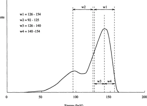
Figure 2-1: Definition of the energy window settings overlaid on an energy spectrum of Tc99m photon source. Note that this energy spectrum is only an example. The actual energy spectrum may vary with the geometry and distribution of the object and source, the distance between the collimator and the source, etc.

The dual-energy window method [8, 9] assumes that the spatial distribution of the scattered photons detected in the photopeak window (usually set at 126 - 154 keV, wl in Figure 2-1) can be estimated as k times the spatial distribution of the photons detected in a secondary (scatter) window which is placed over the Compton part of the energy spectrum (Figure 2-1).

Spk=

kIc

(2.1)

where Spk is the scatter component included in the image reconstructed using events acquired in the photopeak window, I is the image reconstructed using events acquired in the secondary window. The secondary window is set at 92 - 125 keV (w2 in Figure 2-1) in this study as originally suggested [8] (some investigators [10, 11] have examined this method by setting the scatter window at 100-120 keV in order to totally exclude all primary photons). The scatter-free image is then estimated as:

(20)

Upk(i)

= I(i) -

Spk(i)

(2.2)

where I is the reconstructed image derived from the photopeak window.

In Jaszczak's study [8], two Tc99m line sources with identical 5 mm diameter and 5 cm length were imaged in air and in a water-filled cylindrical phantom with a diameter of 22 cm. k value was optimized to be 0.5 which resulted in a compensated line source image whose count rates were within 10% of the count rates of the image of the line source in air. An extended-source distribution phantom and a patient were used to evaluate this compensation method. The phantom consisted of six solid acrylic spheres (diameter 10, 13, 16, 19, 25, 32 mm) placed within a cylindrical (22 cm diameter) distribution of Tc99m. For sphere diameters greater than 25 mm the measured image contrasts were within 8% of the true uptake ratios. For the other four spheres, the measured image contrasts were beyond 10% of the true uptake ratios. Compensated liver/spleen SPECT images of patient with small posterior filling defect in liver also showed improvement in quantification.

In practice, scatter correction can be performed on the projection images (before image reconstruction) or on the reconstructed images (after image reconstruction). The former requires only one reconstruction procedure while the latter requires two reconstruction procedures.

2.1.2 Dual-Photopeak Window Method

The dual-photopeak window method [12] assumes a relationship between the ratio of scattered photons to unscattered photons in pixel i in the photopeak window, SUR(i), and the ratio of the number of counts detected in two equally wide subwindows splitting the photopeak window (w3 and w4 in Figure 2-1):

SUR(i) = A{ (i) } + C (2.3) I2I (i)

where I, (i) and I,, (i) are the numbers of counts detected in the lower and upper windows in the pixel i. A, B, and C can be calibrated by nonlinear regression analysis.

(21)

Then the scattered number of photons in the photopeak can be estimated as: SUR(i)

Spk(i) = I(i) SUR(i) (2.4)

1 + SUR(i)

where I(i) = Ilw(i) + I ,(i). The estimated image of unscattered photons in the photopeak window is then:

Upk(i)

=

1(i)

-

Spk(i)

(2.5)

In King's study [12], this idea was tested by acquiring dual photopeak window acquisitions of a Tc99m point source in an elliptical attenuator, and at the same location in air. From these, the regression constants A, B, and C were then deter-mined. In SPECT acquisitions, this method was observed to significantly increase the contrast of cold spheres of a so-called Data Spectrum phantom, and improve the accuracy of estimating activity at the center of hot spheres.

The major shortcoming of DPW is that for low count projection images, the scatter estimate will be quite noisy since in this case SUR(i) and R(i) might vary greatly from one pixel to another pixel, making their regression relationship unreliable.

2.1.3 Channel Ratio Method

The same two subwindows that split the photopeak window as used in the above method are used in the channel ratio method. This method [6] assumes that the ratio of the number of unscattered photons detected in these two subwindows is constant as well as the ratio of the number of scattered photons:

U~(i) - G _(2.6)

UW (i)

S•=(i) H (2.7)

Suw (i)

where U and S stand for unscattered and scattered respectively, 1w and uw rep-resent the lower window and upper window respectively.

(22)

The number of counts detected in the lower and upper windows are:

IW (i) = UW (i) + S1W(i) (2.8)

,(i)W = U, W(i) + S,(i) W(2.9)

Then the estimated number of unscattered photons in the photopeak window can be expressed by:

1+G

Upk(i) = H[IIw(i) - HIuw(i)] (2.10)

G-H

In practice, to determine the values of G and H, G(i) = U~,(i)/Uw,(i) and H(i) =

Sil(i)/S,,(i) are calculated for each pixel in the projection images. G and H are then chosen as the mean values of the G(i) and H(i) values respectively.

This method was proved to be able to improve image resolution [6]. Results showed a 30.4% improvement in the geometrical resolution defined as the full width at tenth maximum of a line source at a depth of 150 mm water. This method was also tested on clinical planar liver and bone images. Improved contrast with increased noise level could be identified by visual inspection.

Some points need to be mentioned for channel ratio method.

* The value of G depends on the energy stability of the gamma camera. It has been found that a drift of 0.5 keV could effect the G value by approximately 10% which corresponds to an error of roughly 10% in the final quantitation [6]. * The size and the depth of the sources could influence the value of H. The H value

measured for the small source was found significantly less than those of large sources [6]. And photons closer to the surface undergo less Compton scattering and yield smaller H.

* Total breakdown of the channel ratio method could occur when only scattered photons and no unscattered photons are included in the ROI. But it can be

(23)

counts I ) I I I PW I ~---, I I 1ppro. )pro. 0 50 100 150 200 Energy (keV)

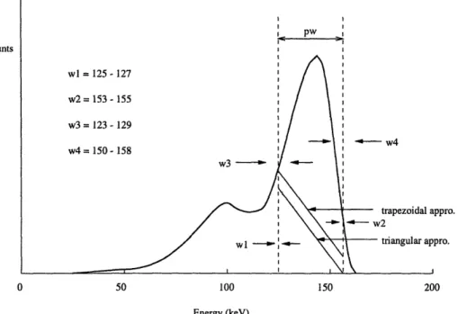
Figure 2-2: Definition of the energy window settings of three-window methods of using trapezoidal approximation and triangular approximation.

avoided easily since this situation only applies to the region outside of the edge of an organ/phantom.

No real camera is involved in this simulation study, G and H will be properly calibrated for the studied phantom, and ROI region will be selected to contain both scattered and unscattered photons, thus none of the above three factors will influence the implementation of CRM scatter correction in this study.

2.1.4 Three-Window Method Using Trapezoidal

Approxi-mation

The three-window method using trapezoidal approximation [13] assumes that the scatter component energy spectrum in the photopeak can be estimated by the trape-zoidal area (Figure 2-2) located under the linear fit between the number of photons

I (i) and I2(i) detected at energies El and E2 which are located right on both sides

of the photopeak. In practice, II(i) and I2(i) are estimated by acquiring two narrow

(24)

scattered photons in the photopeak is then:

Spk(i) = [I (i)+ I 2(i)]

_2w,

(2.11)

where w and w, are the widths of the photopeak and narrow windows. Two 2 keV narrow windows are used, centered on 126 and 154 keV respectively.

Three cylindrical phantoms [13] were tested using this scatter correction method. The first phantom contained uniform source. The second phantom was uniformly source-filled except inside a small cylinder which was filled with only water. The third phantom was water filled except inside a small cylinder which is filled with source. The diameters of the large cylinder and the small cylinder were 20 cm and 6 cm, respectively. The axis of the small cylinder was 5 cm away from that of the large cylinder. Profile curves of the reconstructed images after scatter correction for those three phantoms showed good agreement with the corresponding ideal images reconstructed using true unscattered photons.

2.1.5 Three-Window Method Using Triangular

Approxima-tion

In the three-window method using triangular approximation [14], photons in two narrow windows similar to those in the above method are acquired (w3 and w4 in Figure 2-2). However, the scatter component is estimated by, instead of the area of a trapezoid, the area of a right triangle with a height equal to the estimated number of scattered photons at photopeak lower-edge energy El (Figure 2-2).

This method assumes that the photons detected at photopeak upper-edge energy E2 are only unscattered photons, and the photopeak is symmetric around the emission

energy Eo if there is no scatter, i.e.,

(25)

Ui(i) = U2(i)

Then the number of scattered photons in the lower narrow window can be esti-mated as:

S1 (i) = I (i) - U (i) = i (i) - U2(i) = I1(i) - 12(i) (2.14)

The number of scattered photons detected in the photopeak is then:

In

(i)

In

2

Spk(i) =

i)

(2.15)

Wnl Wn2 2

These two narrow windows wl and wn2 are usually set at 123 - 129 keV and 150 - 158 keV.

The phantom tested on this scatter correction method consisted of four identical 4 cm high and 3 cm diameter cylinders embedded in a 21.8 cm high and 22 cm diameter cylindrical phantom containing a uniform background of Tc99m [14]. Relative Tc99m activity concentrations of the four hot small cylinders with respect to the background were 2, 4, 6 and 8, respectively. The scatter corrected projection image of this phan-tom was evaluated for quantitative accuracy. While no values were provided, a figure showing measured relative activities in each of the small cylinders indicated almost 100% accuracy except a slight overprediction of source strength in the hottest small cylinder.

2.2 Spatial Analysis Methods

2.2.1 Spatial Analysis Methods Based On the Line Spread

Function

Spatial analysis methods based on the line spread function assume that the measured projections P are considered to be the sum of a nonscatter component N and a scatter component S:

(26)

P=S+N

The scatter component S is modeled as a convolution of a simple blurring function E, usually an exponential function, with some projection distribution X:

S=X E (2.17)

The blurring function E is determined from the shape of Line Spread Function which is obtained by acquiring projection images of a line source located in the same scattering medium. The detailed procedure to get the line spread function and the exponential function will be described later.

Note that the deconvolution is performed prior to reconstruction.

Axelsson method

Scatter is modeled as the convolution of the measured (scatter + unscatter) projection data P with the exponential function E [15].

S=P E (2.18)

Then this estimate of the scatter is subtracted from the acquired projection to provide the compensated projection PC:

Pc = P - S (2.19)

The accuracy of this method was tested on a simple phantom simulating a SPECT investigation of the liver [15]. The indicated ratio of the activity concentration in a photon-deficient area, 60 mm diameter in the "liver", relative to its surroundings, was 0.28/1 without scatter correction and 0.01/1 with the scatter correction.

(27)

Floyd method

Scatter is modeled as the convolution of the nonscatter projection data N with the exponential function E [16].

S=N E (2.20)

Since P = S + N, we can get

P = N ®E + N = NO (E + 6) (2.21)

where 6 is Dirac delta function.

Express the equation in terms of Fourier Transformation

FT[P] = FT[N]FT[6 + E] (2.22)

Solving for N yields

N = FT-I( FT[P] (2.23)

FT[6 + E]

This deconvolution technique has been evaluated for several phantoms [16]. The line source phantom consisted of a 0.5 cm diameter and 11 cm length line source located at or 5 cm away from the axis of a 22 cm diameter and 11 cm length water filled cylinder. Using the deconvolution scatter correction, the resulting reconstructed images of the line source both on-axis and 5 cm off-axis showed a good agreement with those resulting from projections containing only unscattered photons. In another experiment, contrast of the cold spot was improved by 12% for a phantom consisting of a 6.3 cold-sphere immersed in 22 cm diameter active cylinder. Also, an improvement in lesion contrast was apparent in a clinical image of a liver having a cold lesion defect.

(28)

2.2.2 Spatial Analysis Methods Based On the Point Spread

Function

Data are first collected in a photopeak window from a point source located in the scattering medium. The shape of the point spread function (PSF) obtained is due to the physical dimensions of the collimator and to the inclusion of scattered photons in the data. It is assumed that deconvolving this function from a subsequent acquisition will thus compensate not only for the geometric response of the collimator, but also for the effects of the scattered photons.

2D PSF deconvolution

Deconvolution of a 2D measured PSF h(x, y) from each frame of projection data p(x, y) prior to reconstruction [11].

p(x, y) = o(x, y) 0 h(x, y) (2.24)

where o(x, y) is the true projection without scattered component. After the Fourier Transformation,

P(u, v) = O(u, v)H(u, v) (2.25)

Direct inversion to obtain O(u, v) will lead to large fluctuation in the estimate of the object distribution due to the existence of very small values in the FT of the PSF. So a constrained deconvolution is necessary.

O(u, v) = P(u, v)W(u, v) (2.26)

H*

WH(u, v) = (2.27)

iH2(U, V)

I

+

Here y is held constant. The function W(u, v) is a modification of the Wiener filter in which 7 depends on frequency and represents the ratio of the power spectrum

(29)

of noise to that of signal. Because these spectra are difficult to determine in practice, modifying the filter by keeping 7 fixed becomes a practically useful approximation. The optimal value of 7 is chosen so as to produce a satisfactory improvement in image contrast (to be defined in Chapter 3) without creating undesirable levels of image mottle (to be defined in Chapter 3).

One cold-spot hot-background phantom and one cold-spot resolution phantom were tested on this scatter correction method [11]. The cold-spot hot-background phantom consisted of a 19 cm diameter and 12 cm thick Tc99m source filled cylindri-cal phantom within which five water filled cylinders were placed at the same radial position (6.0 cm from the center) and each cylinder had equal outer heights and di-ameters of 5, 4, 3, 2, and 1 cm. The scatter correction using the proposed technique resulted in about 30%, and 10% improvements for the four smaller cold spots and the larger two cold spots, respectively. The resolution phantom consisted of a 21 cm diameter and 20 cm high Tc99m source filled cylinder containing a pie-shaped "cold rod" insert. The diameters of the cold spots in the insert were 1.55, 1.25, 0,95, 0,80, and 0.55 cm. The deconvolution technique successfully resolved the 1.55 cm cold spots.

3D PSF deconvolution

The 3D PSF deconvolution involves deconvolution of a 3D measured PSF h(x, y, z) from a stack of reconstructed slices r(x, y, z) [11].

r(x, y, z) = o(x, y, z) 0 h(x, y, z)

(2.28)

where o(x, y, z) is the original 3D source distribution.

The constrained deconvolution follows the same procedure described in the above method.

This deconvolution technique was tested using the same cold-spot hot-background phantom and resolution phantom as those in the 2D PSF deconvolution technique [11]. Image contrast for each cold spot in the cold-spot hot-background phantom was

(30)

improved by 10% to 25%. In the resolution phantom, both 1.55 cm cold spots and 1.25 cm cold spots were resolved.

2.3 Other Methods

2.3.1 The Simplest Scatter Correction

While the attenuation due to photoelectric absorption removes gamma photons from the ray sum, resulting in a decrease in the counts detected, the Compton scattering results in additional photons which carry misleading information of photon source. Thus the simplest way of correcting for scatter is to undercorrect for attenuation [17], that is, to use an effective value of attenuation coefficient A in the correction for photon attenuation (typically 0.13 cm- 1 _{instead of 0.15 cm}- 1 _{for 140 keV photons of}

Tc99m in a water-filled object). Obviously this approach is not quantitative, since it ignores the dependence of scattered photons on the three-dimensional source and attenuation distribution.

2.3.2 Several Other Spectral Analysis Methods

The photopeak energy distribution analysis method [18] relies on the assumption that the photopeak window can be divided into two subwindows so that for any pixel, the number of scattered photons detected within these subwindows are equal. The scatter correction consists of subtracting the image acquired in the lower window from that corresponding to the upper window. The only parameter to be determined is the cut-off energy between these two windows. This method was proved to be nonquantitative because the corrected image is very noisy due to the method's inherent removal of many unscattered photons [14]. In another spectral analysis method [19] the energy spectrum detected at each image pixel is used to estimate the scatter contribution spectrum. The scatter spectrum can be modeled as a polynomial function of energy channel bins. Parameters are chosen by least square fitting technique. Finally, the Gaussian scatter correction method [20] is based on the fact that the energy spectral

(31)

peak would be basically Gaussian in shape if there is no scatter. A Gaussian function is fitted to the the photopeak's upper energy portion which is assumed to be relatively scatter free. Then the Gaussian function can be used to estimate the number of good counts within the photopeak window.

2.3.3 Several Other Multiple Energy Window Methods

There are several other multiple energy window methods in addition to those two three-window methods described before. An energy-weighted acquisition (EWA) tech-nique acquires data from multiple energy windows. The images reconstructed from these data are weighted with energy-dependent factors to minimize scatter contribu-tion to the weighted image [21]. The holospectral imaging method [22] estimates the scatter contribution from a series of eigenimages derived from images reconstructed from data obtained from a series of multiple energy windows. The use of multiple en-ergy windows may create practical problems for clinical implementation since some of today's gamma cameras are unable to correct for linearity (i.e., the linear relationship between the energy of a detected photon and the corresponding "z signal" described in section 1.1.1) separately in many different energy windows.

2.3.4 Methods Based On Nonstationary Assumptions

Another class of methods try to characterize the exact scatter response function and incorporate it into iterative reconstruction algorithms for accurate compensation for scatter [16, 23, 24, 25]. Since the exact scatter response functions are nonstationary (i.e., they are dependent upon source distribution, scattering material, object size, source location in object, distance and angle of detector, etc.), implementation of the methods requires extensive computations. However, efforts are being made to parameterize the scatter response function and optimize the algorithm for substantial reduction in processing time [25, 26]. In general, the use of this type of method produces a better scatter correction than those based on stationary assumptions, but in most cases the results still do not match the source distribution precisely.

(32)

Chapter 3 Approach

3.1 SimSPECT

3.1.1 Simulation study of SPECT

Clinical images produced by SPECT imaging systems are inherently noisier and of lower resolution than images from such modalities as MRI or CT, due to numerous fac-tors including attenuation and scatter in the object, the geometry and composition of the collimator, and the controllable imaging parameters, such as source-to-detector distance, energy windows, and energy resolution in the gamma camera. Unfortu-nately, the effects of these factors cannot be easily studied in an experimental setting because of cost or physical limitation. One alternative way to study such effects is to perform simulations of the entire SPECT imaging situation. Such simulations can provide data (via synthetic images) that can be used to individually examine the origins of degradation of SPECT images, to design methods to mitigate such effects (scatter correction and attenuation correction algorithms, etc), and to analyze new imaging systems regarding feasibility and performance characteristics.

3.1.2 Introduction to SimSPECT

A sophisticated SPECT Simulation system named SimSPECT has been devel-oped at the MIT Whitaker College Biomedical Imaging and Computation

(33)

Labora-tory(WCBICL) [27, 28]. The SimSPECT system is based on MCNP (Monte Carlo Neutron-Photon transport code) [29] which has been extensively modified to allow realistic modelling of the geometry and composition of source, object, and collima-tor, photon transport and interaction with media, and other geometric and physical parameters of SPECT imaging situation such as the distance between object and col-limator,number of views, etc. Detailed descriptions and validations of SimSPECT can be found in [27, 28].

The output of SimSPECT is synthetic projection image data stored in so-called ListMode files, each of which corresponds to a projection view at a certain angle.

A ListMode file stores, in a sequential list, detailed information of every photon

reaching the face of a virtual detection crystal, including energy, x and y position of interaction with the detection plane, the number of scattering interactions in the object and transport medium, and the number of scattering interactions in the colli-mator.

With SimSPECT, it is possible to distinguish scattered from unscattered photons and to generate scatter-free projection images which could act as a standard to allow an objective assessment of the performance of different scatter correction methods. In addition, ListMode data can be assorted conveniently to generate projection images containing photons which have any user-defined scatter order and are acquired in any user-defined energy window, making the testing of the assumptions of each scatter correction method feasible.

3.2 Phantoms and Simulation

In order to make a comparative assessment of different scatter correction methods, certain phantom simulations are needed to provide projection images for scatter cor-rection. The advantage of phantom simulation is that source distribution, scattering medium distribution and object size are known exactly, providing objective standards for evaluation of different scatter correction methods. In this study, a cold-spot hot-background phantom is used to provide evaluation of each scatter correction method's

(34)

19.9 cm

8 cm

Figure 3-1: The cold-spot hot-background phantom. The right is the cross sectional image at the center plane (with a height of 4 cm) of the left cylinder.

ability to improve image contrast (to be defined below) and influence on image mot-tle (to be defined below), another hot-spot cold-background phantom is employed to examine each scatter correction method's potential of image resolution improvement.

3.2.1 Cold-spot hot-background phantom

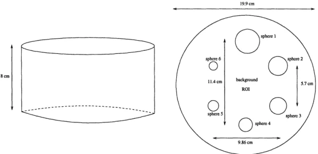
The cold-spot hot-background phantom used in this study (Figure 3-1) is a 19.9 cm-diameter and 8 cm-thick Tc99m uniformly filled cylinder with six water-filled spheres of different radii located at different positions inside it.

The radii of spheres 1, 2, 3, 4, 5 and 6 are 1.59 cm, 1.27 cm, 0.995 cm, 0.795 cm, 0.635 cm and 0.475 cm, respectively. The center of each sphere is located at the plane of half thickness of the cylinder.

In the SimSPECT simulation, the radius of camera rotation is 16 cm. Sixty projections are obtained at equally spaced angles over 3600. The collimator simulated has a 39 diameter field of view, containing 85474 0.111 diameter and 2.36 cm-long hexagonal parallel holes. All of the following phantom simulations use the same radius of rotation, number of projections and collimator dimension.

The SimSPECT simulation of this cold-spot hot-background phantom took nearly

_L

(35)

---19.9 cm

8 cm

3.8 cm

location of the slice of interest

0.2 cm source slice

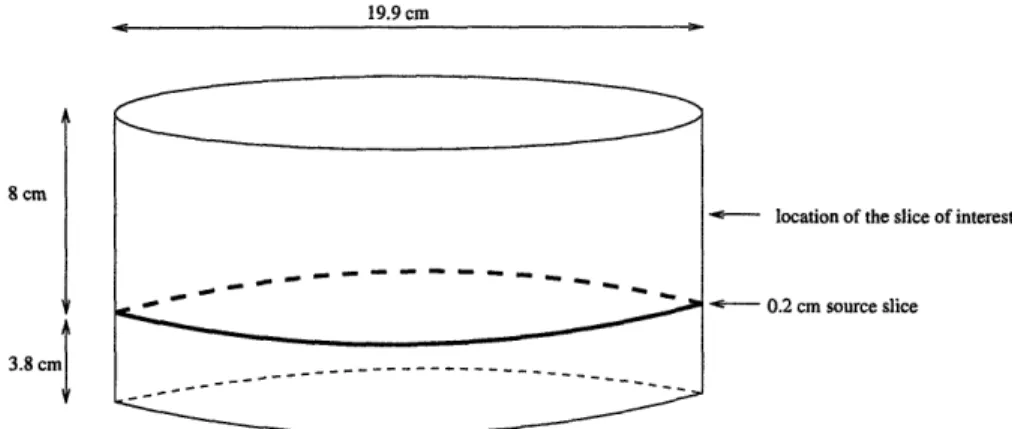
Figure 3-2: The extended cylinder phantom used for validation of the old-spot hot-background phantom.

three months to obtain 60 projection images containing about 970,000 photons in each. We see here that the MCNP simulation is very time-consuming.

3.2.2 Validation of the cold-spot hot-background phantom

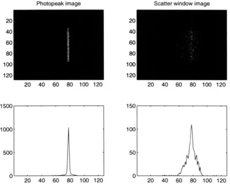
In order to save simulation time, the height of the above cold-spot hot-background phantom is set as 8 cm which is less than the size of a typical clinical phantom (e.g., a human brain has an average diameter of about 16 cm). In addition, the mean free path of a 140 keV photon in water is about 6.7 cm, making it possible that some of the photons originating more than 4 cm away from the center slice of the cold cylinder could contribute to the scatter component detected at the center slice. So a validation of this 8 cm-high phantom is necessary. A new phantom (Figure 3-2) is created based on the original phantom. A 0.2 cm-thick slice of Tc99m source and 3.8 cm-thick slice of water are added to the bottom of the original 8 cm-high cylinder which is now homogeneously filled with water without any Tc99m source included. Figure 3-3 shows a projection image (128 x 128) acquired through the photopeak window, and a projection image (128 x 128) acquired through the scatter window which is set as 92 keV-125 keV, as well as their projection profiles. Since slice 64

~---~---~, · r s -- --- ---- --- _~

(36)

Scatter window image 2( 4( 6( 8( 10( 12( 20 40 60 80 100 120 20 40 60 80 100 120 1500 1000 500

0

1 20 40 60 80 100 120 20 40 60 80 100 120

Figure 3-3: The projection images through photopeak window and scatter window and their projection profiles.

and slice 65 are the central slices where the cold spheres are located, the scatter contribution originating more than 4 cm away to the total scatter detected in these two slices is concerned. In order to calculate the sum of the scatter contribution from slices inside the 4 cm region and outside the 4 cm region, the projection profile is assumed uniform along the slice bin, then each slice's individual contribution to the scattered photons acquired in the slice of interest (slice 64 or 65) can be estimated and summed. The results show that about 1% of the scattered photons contributing to the photopeak window at the slice of interest actually originate at distances greater than 4 cm away from the slice of interest, while the corresponding percentage for the scatter window is about 3%. The influence of these photons is not significant in the case of photopeak window acquisition. However, in the case of scatter window acquisition, attention should be paid to those scatter correction methods which result in image quality improvements with slight differences (i.e., comparable to 3%) because the error induced by inappropriate phantom geometry may overshadow the true differences between scatter correction methods.

Photopeak image

"^^

(37)

ff

i

-X.

-

i

Figure 3-4: The cross-sectional image of the resolution phantom as generated using MCNP's internal plotting routine.

3.2.3 Resolution phantom

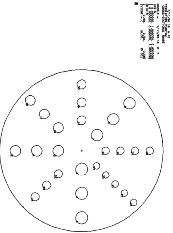
The resolution phantom used in this study is a hot-spot cold-background phantom (Figure 3-4). The centers of all the Tc99m filled spheres are located on the center plane (with a height of 4 cm) of a 19.9 cm-diameter and 8 cm-high water-filled cylin-der. They are divided into eight groups. Spheres of the same group have the same diameter. Intervals between spheres of the same group equal the diameter of that group. Radii of the spheres are 0.75 cm (spheres 4, 5, 6), 0.70 cm (spheres 7, 8, 9), 0.65 cm (spheres 10, 11, 12), 0.60 cm (spheres 14, 15, 16), 0.55 cm (spheres 18, 19, 20), 0.50 cm (spheres 22, 23, 24), 0.45 cm (spheres 25, 26, 27, 28), and 0.40 cm (spheres 29, 30, 31, 32, 33).

The result of this SimSPECT simulation gives 60 projection images containing about 47,000 counts for each.

(38)

3.2.4 Line spread function (LSF) phantom

The line spread function required for the Axelsson LSF convolution method and the Floyd LSF deconvolution method is obtained by simulating a 0.2 cm-diameter and 6 cm-long Tc99m line source located on the cylindrical axis of the 19.9 cm-diameter and a 8 cm-high water-filled cylinder. The resulted projections contain about 10,000 counts for each.

3.2.5 Point spread function (PSF) phantom

The point spread function required for the 2D and 3D PSF deconvolution methods is obtained by simulating a Tc99m point source located at the center of the water-filled cylinder described above. The resulted projections contain about 10,000 counts for each.

3.3 Computation Techniques

The scatter correction methods are programmed as Matlab functions. The compar-ison and analysis are also performed in the Matlab environment. The SPECT im-age reconstruction is carried out using filtered backprojection reconstruction with the Hann filter [30] (see below) supplied within the Donner Algorithms for Reconstruction Tomography [31]. The interfaces between SimSPECT, Matlab, and Donner Algo-rithms are programmed in C. Chang's attenuation correction method [32] is used to correct for attenuation (see below).

3.3.1 Filtered backprojection reconstruction with the Hann

filter

The filtered backprojection (FB) algorithm [30] is the most frequently used recon-struction method for SPECT imaging systems. The algorithm with the Hann filter consists of four steps:

(39)

2. Multiply by the Hann filter. 3. Take inverse Fourier transform.

4. Backproject to get reconstructed image.

The procedure can also be described by the expression:

rimage = backproject{FT- {Hann -FT{projection}}} (3.1)

where rimage is the reconstructed image, Hann is the Hann filter. The Hann filter is defined by the equation:

Hann(f)

/Ifl [0.5 + 0.5cos(7rf/

f

m

)] if

If

I

5 fm

Hann(f) = 0(3.2)

0 if ifI >fm

where fm is the cutoff frequency. The Hann filter usually results in a good SNR level in the reconstructed image with a loss in resolution.

The cutoff frequency is chosen as 0.23 cycles/pixel, or 0.77 cycles/cm for 128 x 128 projection images acquired on a 39 cm by 39 cm square detector plane, for all the reconstructions carried out for the the cold-spot hot-background phantom. For the recontructions associated with the resolution phantom, the cutoff frequency is chosen as 0.5 cycles/pixel, or 1.67 cycles/cm.

3.3.2 Chang's attenuation correction method

Chang's attenuation correction method [32] assumes a uniform attenuation coefficient over the object being imaged. It requires knowledge of the attenuation coefficient and the body contour. The measured projection data are first reconstructed without attenuation compensation. A correction factor is calculated at each image point as the average attenuation factor over all projection angles. The correction factor for attenuation at point (xo, Yo) is defined by:

1

c(xo,yo) = ±

(-

(3.3)

1 e39 xp(-Aloi)

(40)

where M is the total number of projections taken in a 3600 scan measurement, Iu is the uniform attenuation coefficient, 10i is the distance between point (xo, yo) and the boundary point of the medium at projection angle Oi. The reconstructed image is multiplied by the correction factors to compensate for attenuation. An iterative scheme in which the primary corrected image is reprojected to form a new set of pro-jections leading to an error image to be added to the primary corrected image to form a final image can also be implemented to improve the accuracy of the compensation. Since the shapes of all phantoms simulated in this study are known, and they contain uniform medium (water with attenuation coefficient 0.15 cm-1), selecting Chang's method as the attenuation correction is suitable.

3.4 Assessment Criteria

3.4.1 Image Contrast

Image contrast is assessed for the six cold spots in the cold-spot hot-background phantom (Figure 3-1) for each scatter correction method. Image contrast is defined as the difference in reconstructed count density in the cold spot ROI and the count density in the background ROI, divided by the latter. The ROI for each cold spot consists of all the pixels located inside the circle of that cold spot. The ROI sizes for cold spot 1, 2, 3, 4, 5 and 6 are 84, 55, 34, 20, 14 and 7 pixels, respectively. The background ROI (Figure 3-1) is a square covering the area ranging from row 58 and column 58 to row 71 and column 71 in a 128 x 128 reconstructed image, containing totally 196 pixels.

3.4.2 Statistical error estimation in image contrast

Due to the Poisson counting fluctuation associated with counts detected in each pixel, the calculation of image contrast must include the statistical error estimation using the statistical error propagation theories [33]. Suppose u represents one cold spot's contrast, t represents the mean pixel value of the ROI of that cold spot, 9 represents

(41)

the mean pixel value of the ROI of the background, d represents the difference between Z and 9, and ua, at, ad, d represent the statistical error of u, x, y and d, respectively.

Then we have

d = - (3.4)

ad2 =

Ut2

+ aU2

(3.5)

d

= - (3.6)

a)2 d )2 _{9 2} (3.7)

u d y

=-

(=-Ud))

+(Y)

(3.8)

The statistical error of t and 9, are estimated as:

a = N (3.9)

N

a = V M (3.10)

where N and M are the total number of pixels in the cold spot's ROI and the background ROI, respectively.

3.4.3 Image Mottle

Image mottle, also assessed for the cold-spot hot-background phantom, is calculated as the ratio of the standard deviation of pixel values to the mean pixel value in the background ROI.

(42)

3.4.4 Resolution

Assessment of resolution is based on visual inspection and profile drawing of the hot-spot cold-background resolution phantom. Groups of smaller hot hot-spots differentiated indicate better resolution. To make the resolution evaluation more quantitative, we can calculate the contrast of the valleys between each two neighboring peaks on the profile through a hot spot group which is not quite resolved. The contrast is defined as the difference between the height of a valley and the height of its lower neighboring peak, divided by the latter. The higher contrast values for each valley imply better image resolution.

3.4.5 Ease of implementation

The ease of implementation is assessed in terms of the number of energy windows required, the parameter calibration required, and the computational complexity in-volved in scatter correction procedure.

(43)

Chapter 4 Results and Analysis

4.1 Dual-Energy Window Method (DEW)

The value of constant k in equation (2.1), the fraction of the images derived from the scatter window to be subtracted from the images derived from the photopeak window (PW), plays a key role in the dual-energy window (DEW) method. Though a value of 0.5 is originally suggested for k [8], it have been tested for only limited number of phantoms. The optimal value of k should depend on individual phantom and imaging situation.

Instead of imaging line sources in air and water as was done by Jaszczak [8], this study starts from building a histogram of k values in each pixel to determine the mean value of k. SimSPECT can generate projection images consisting of only scattered photons included in the photopeak window for the cold-spot hot-background phantom. Then we can calculate the ratio of each pixel value of a typical projection image acquired through the scatter window and the corresponding pixel value of the true scatter projection image to yield a histogram of k. Figure 4-1 shows the histogram of k within a typical projection image's ROI (35:94, 53:76) which covers the area from row 35 to row 94 and from column 53 to column 76 (Figure 4-2), containing 2,400 pixels. This ROI matches the projection of the 8 cm-high 19.9 cm-diameter cylinder to the detection plane which is a 39 cm by 39 cm square. The k value ranges from the minimum 0.4601 to the maximum 0.7738 with a mean value of 0.6062 and a standard

(44)

Figure 4-1: Histogram of k within the ROI of a typical projection image.

2u 4U bU U 1TUJ 12z

Figure 4-2: A typical projection image (128 x 128) of the cold-spot hot-background phantom.

Comparative assessment of several SPECT scatter correction methods using SimSPECT

Comparative Assessment of Several SPECT

Scatter Correction Methods using SimSPECT

by

An Lu

Submitted to the Department of Nuclear Engineering

in partial fulfillment of the requirements for the degree of

Master of Science in Nuclear Engineering

at the

MASSACHUSETTS INSTITUTE OF TECHNOLOGY

September 1996

©

Massachusetts Institute of Technology 1996. All rights reserved.

A uthor ...

.. . ... . ...

Department of Nuclear Engineering

August 23, 1996

Certified by....

J. C. Yanch

Professor

s Supervisor

Certified b.

A. B. Dobrzeniecki

Research Scientist

Thesis Supervisor

Accepted by ...

Chairman,

/ I/ -

J. Freidberg

Departmental Committee on Graduate Students

MAY 19 1997

$1

Comparative Assessment of Several SPECT Scatter

Correction Methods using SimSPECT

by

An Lu

Abstract

Acknowledgments

Contents

List of Figures

List of Tables

Chapter 1

Introduction

1.1

Nuclear Medicine and SPECT

I I I I I I I

I

I I

I

I

I I

I

I

I

I

I I I I I I

it

1.1.2

PET and SPECT

1.2

Scatter problem in SPECT

1.3

The rest of this thesis

Chapter 2

SPECT Scatter Correction

Methods

2.1

Energy Window Methods

Spk=

kIc

(2.1)

Upk(i)

= I(i) -

Spk(i)

(2.2)

2.1.2

Dual-Photopeak Window Method

1 + SUR(i)

Upk(i)

=

_2w,