Compressive sensor networks : fundamental limits and algorithms

(1)

Compressive Sensor Networks:

Fundamental Limits and Algorithms

by

John Zheng Sun

B.S. Electrical and Computer Engineering, Cornell University (2007)

Submitted to the Department of Electrical Engineering and Computer

Science

in partial fulfillment of the requirements for the degree of

Master of Science in Electrical Engineering and Computer Science

at the

MASSACHUSETTS INSTITUTE OF TECHNOLOGY

September 2009

@

John Zheng Sun, MMIX. All rights reserved.

The author hereby grants to MIT permission to reproduce and

distribute publicly paper and electronic copies of this thesis document

in

whole

or in part.

MASSACHUSETTS

TNSTITUTE

OF TECHNOLOGY

A

SEP 3 0 2009

LIBRARIES

A u th or

... ./ ... . ... ...

Department of Elctrical Engineering and Computer Science

i

ASeptember

2, 2009

Certified by

...

v1".

'

L.

".. .

e

...

Vivek K Goyal

Esther and Harold E. Edgerton Associate Professor of Electrical

Engineering

Thesis Supervisor

A

ccepted by ... ,...

... ...

Terry P. Orlando

Chairman, Department Committee on Graduate Theses

(2)

(3)

Compressive Sensor Networks:

Fundamental Limits and Algorithms

by

John Zheng Sun

Submitted to the Department of Electrical Engineering and Computer Science on September 2, 2009, in partial fulfillment of the

requirements for the degree of

Master of Science in Electrical Engineering and Computer Science

Abstract

Compressed sensing is a non-adaptive compression method that takes advantage of natural sparsity at the input and is fast gaining relevance to both researchers and engineers for its universality and applicability. First developed by Candis et al., the subject has seen a surge of high-quality results both in its theory and applica-tions. This thesis extends compressed sensing ideas to sensor networks and other bandwidth-constrained communication systems. In particular, we explore the limits of performance of compressive sensor networks in relation to fundamental operations such as quantization and parameter estimation.

Since compressed sensing is originally formulated as a real-valued problem, quanti-zation of the measurements is a very natural extension. Although several researchers have proposed modified reconstruction methods that mitigate quantization noise for a fixed quantizer, the optimal design of such quantizers is still unknown. We propose to find the optimal quantizer in terms of minimizing quantization error by using recent results in functional scalar quantization. The best quantizer in this case is not the optimal design for the measurements themselves but rather is reweighted by a factor we call the sensitivity. Numerical results demonstrate a constant-factor improvement in the fixed-rate case.

Parameter estimation is an important goal of many sensing systems since users often care about some function of the data rather than the data itself. Thus, it is of interest to see how efficiently nodes using compressed sensing can estimate a parameter, and if the measurements scalings can be less restrictive than the bounds in the literature. We explore this problem for time difference and angle of arrival, two common methods for source geolocation. We first derive Cramer-Rao lower bounds for both parameters and show that a practical block-OMP estimator can be relatively efficient for signal reconstruction. However, there is a large gap between theory and practice for time difference or angle of arrival estimation, which demonstrates the CRB to be an optimistic lower bound for nonlinear estimation. We also find scaling laws 'for time difference estimation in the discrete case. This is strongly related to partial support recovery, and we derive some new sufficient conditions that show a

(4)

very simple reconstruction algorithm can achieve substantially better s alings than full support recovery suggests is possible.

Thesis Supervisor: Vivek K Goyal

(5)

Acknowledgments

Marvin Weisbord once said. "Teamwork is the quintessential contradiction of a society grounded in individual achievement," and these words resonate most strongly in the academic community. In preparing this thesis, I have benefited from the support of many talented and genuinely wonderful people that I wish to acknowledge.

First and foremost, I thank my advisor Vivek Goyal for his advice and mentor-ship. Our numerous discussions have been invaluable and his suggestions are always insightful and revealing.

I also acknowledge the members the STIR group for their helpful comments, friendship and encouragement. Specifically, I thank Lay Varshney for the wealth of his knowledge and important pointers to papers on universal delay estimation, Dan Weller for advice on estimation problems, Vinith Misra for discussions on functional quantization, and Adam Zelinski for providing code for sparsity-enforcing reconstruc-tion algorithms. I also appreciate the help of Eric Strattman on the administrative side.

There are several external collaborators that helped shape aspects of this thesis and I thank them as well. Joel Goodman, Keith Forsythe, Ben Miller, and Andrew Bolstad at Lincoln Laboratory worked with me on the Compressive Sensor Networks project. Sundeep Rangan provided excellent suggestions that led to some proofs on partial support recovery. Ramin Samadani, Mitchell Trott, and John Apostolopoulos of HP Labs were very gracious in hosting me as a Researcher in Residence and helped me better understand estimation performance bounds.

On a more personal level, I am indebted to old and new friends for making the last two years particularly memorable. The most important thanks goes to my parents for teaching me that the quest for knowledge is lifelong and always being supportive. I thank my sister Jenny for her infectious boundless energy, and to Grace for possessing the uncanny ability to make me smile. I am grateful to Jon, Yi Zheng, Mitch and Peter for friendships that defy distance, and to all my new friends that has made MIT as fun as it is enlightening.

(6)

(7)

List of Figures

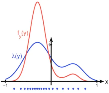
2-1 A source y and its point density function, defined as Ai(t) c( fgY3 (t). A finite-rate quantizer is represented by the dots corresponding to the

placement of codewords. . ... ... 25

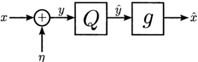
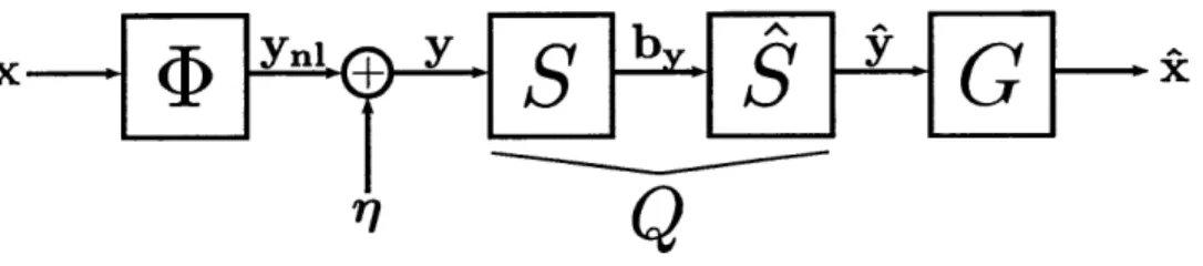
3-1 A compressed sensing model with quantization of noisy measurements y. The vector Ynl denotes the noiseless random measurements. ... 31 3-2 Distribution fy,(t) for (K, M, N) = (5, 71,100). The support of yi

is the range [-K, K], where K is the sparsity of the input signal. However, the probability is only non-negligible for small yi. ... 33 3-3 Estimated sensitivity eys(t) via Monte Carlo trials and importance

sam-pling for (K, M, N) = (5, 71,100). ... .. 37

3-4 Estimated point density functions Acs(t), Aord(t), and Auni(t) for (K, M, N) =

(5,71,100). ... .... ... 38

3-5 Results for distortion-rate for the three quantizers with a 2 = 0.3 and A = .01. We see the sensitive quantizer has the least distortion. . . . 38 3-6 Integration over the circles that form the unit spherical shell for 0 <

0 < arccos(v). ... .. ... 40 3-7 Theoretical versus empirical distribution for different values of M to

validate Lemma 1 ... .... ... ... 42

3-8 Quantization cells of a sensitive quantizer for the function g(yl, Y2) = yl2 ₊_{y12. The cells for larger values of yi are smaller and hence have}

(10)

3-9 Model for scalar lasso example. Assume x is a compressible source and y = x + rl. The measurements are scalar quantized and then used to

reconstruct i through scalar lasso. ... 44

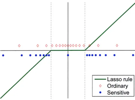
3-10 Scalar lasso and its quantizers. The functional form of lasso is repre-sented by the solid green line and demonstrates lasso shrinkage in that the output has less energy than the input. The ordinary quantizer is

shown in the red diamonds and the sensitive quantizer is represented

by the blue dots. ... ... ... 45

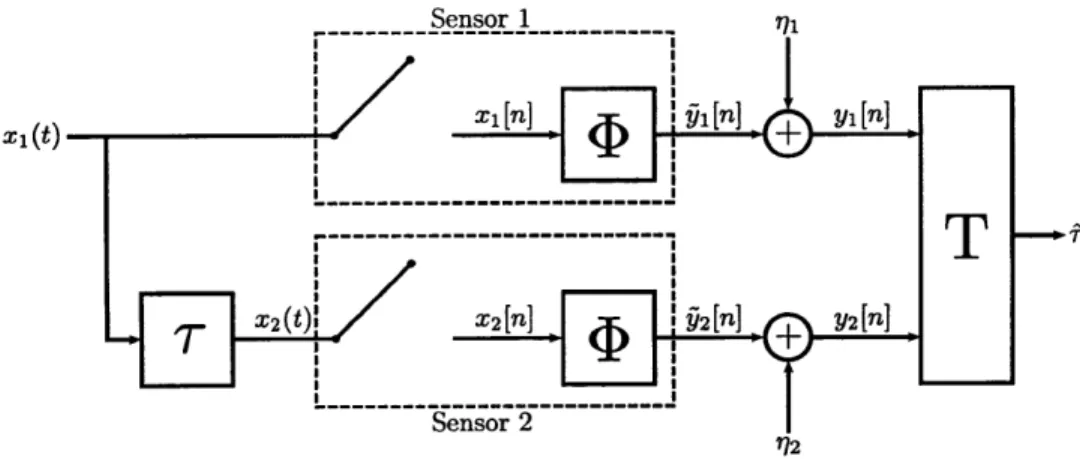
4-1 Problem model for time difference of arrival. The original signal xl (t) and its delayed version z2 (t) are observed by different sensors,

com-pressed using 4, and transmitted in noise. An estimator T determines

the predicted delay . ... . ... . . 49

4-2 CRB for both time difference (TD) and time difference/signal recon-struction (TD/SR) versus OMP experimental error variance for each sampling matrix. We find a large gap between experimental results and the bound. This is because the CRB is optimistic for nonlinear estimation. Other reasons for the loose bounds are discussed. ... 59 4-3 CRB and experimental results with SNR. There is a well-known

phe-nomenon where the estimator performance dramatically deteriorates below a certain SNR. This corresponds to the point where the

cross-correlation begins to fail. ... ... 61

4-4 Experimental error variance versus CRB for signal reconstruction. Since this is a linear estimation problem, the bounds are much tighter than

for time difference estimation. ... ... . . . 62

4-5 AoA problem model. We assume the transmission is sparse in a known basis and satisfy far field and point source approximations. . . . . . 63 4-6 AoA reconstruction performance versus CRB for varying levels of

(11)

5-1 A dTDOA mod(el where the input vectors are compressed through ran-dom projections. The delay r is an element of a discrete set {0, 1,... N}. The estimator T uses (P1 and 12 as side information to find an estimate

. ... ... ... .. 69

5-2 One possible decoder for dTDOA estimation. The lasso/threshold block provides K-sparse estimates with sparsity pattern vectors Ji. The cross-correlation block then finds the delay estimate -. For scal-ings where lasso estimates the sparsity pattern correctly, the estimation

error vanishes with increasing N. ... . 70

5-3 A decoder for dTDOA estimation. The thresholded correlation block has sparsity error rate bounded by 3_{MD through Theorem 5.1. This} can then be approximated using a binary asymmetric channel. The delay estimator is a MMI decoder that succeeds with error vanishing

exponentially. ... . .. ... ... 73

5-4 Modeling the decoder in Figure 5-3 as a noisy channel with MMI esti-mation. The resulting delay estimation error vanishes exponentially. 75 5-5 Numerical simulations for the success of support recovery using TCE.

The color mapping indicates the expected percentage of the support predicted successfully for choices of M and N. The black line indicates the scalings for IMD = 0.4 using Theorem 5.1. . ... . 76 5-6 Numerical simulations of the TCE-MMI delay estimator for /MD = 0.4.

(12)

(13)

Chapter 1 Introduction

Sensor networks are prevalent in today's technological landscape and have inspired important engineering innovations in a variety of military, industrial, and environ-mental applications. However, the nodes of these sensor networks must oftentimes survey wide bands, requiring high-rate analog-to-digital conversion, expensive pro-cessors, and large data flows to propagate information through the network. In the case where the data of interest is sparse in some basis, meaning it has few degrees of freedom, there is an opportunity to filter the measured signal intelligently and use a sub-Nyquist sampling rate while still maintaining the fidelity of the data. Another way of saying this is that it is possible to sample closer to the information rate of the signal rather than being restricted above the Nyquist rate. Moreover, utilizing the underlying sparsity allows for data compression, which eases the communication load between nodes. Efficient techniques for exploiting sparsity in signal representa-tion and estimarepresenta-tion have caused an enthusiastic reexaminarepresenta-tion of data acquisirepresenta-tion in sensor networks.

Compressive sensor networks (CSN) exploit a new compression paradigm called compressed sensing (CS) to non-adaptively filter and compress sparse signals. As described in Section 2.1, CS refers to the estimation of a signal at a resolution higher than the number of data samples by taking advantage of sparsity or compressibility of the signal and randomization in the measurement process. CSN nodes contain analog-to-digital converters (ADCs) that use CS principles such as signal spreading

(14)

and random sampling. This allows the ADCs to sample significantly slower than the Nyquist rate, making the hardware simpler to design and cheaper to manufac-ture. Moreover, we can transmit the compressed version of the input signal and ease communication loads.

This thesis addresses extensions of compressed sensing to quantization and es-timation, both important operations in sensor networks. We focus on fundamental limits and practical algorithms, thereby abstracting out the actual data-collecting machinery. Thus, although the thesis is related to CSN in theme, the questions we study are of independent interest in the compressed sensing literature.

1.1 A Peek at Compressed Sensing

We present a quick summary of compressed sensing (CS) and introduce the nota-tion that will be used in the thesis. We will provide a more detailed look at CS in Section 2.1.

Consider a length-N input vector x that is K-sparse in some orthonormal basis I, such that a length-N vector u = T-1x will have only K nonzero elements. Define the sparsity pattern J to be the set of indices of the nonzero elements in u. Also

define the sparsity ratio to be a " KIN.

Now let a length-M measurement vector be y = 4x, where )E RMXN is the sensing matrix. We define the downsampling rate to be d N/M. In general, since d > 1, we cannot recover x from the measurements y since 1 is underdetermined. The major innovation in compressed sensing for the case of sparse u is that the recovery of x from y via some computationally-tractable reconstruction method can be guaranteed asymptotically almost surely for random sensing matrices (. This means the CS encoder is simply a matrix multiplication, making it linear and non-adaptive. Moreover, the decoder is well-studied and implementable in practice.

Intuitively, compressed sensing works because the information rate is much lower than the Nyquist rate and hence sampling via Shannon's famed theorem is redun-dant. For certain choices of 4), specifically when the sparsity and sampling (T and

(15)

1 respectively) are incoherent, CS provides theoretical bounds on the performance of signal or sparsity pattern recovery.

Many practical reconstruction methods, or decoders, have been proposed including convex programs like basis pursuit and greedy algorithms like orthogonal matching pursuit (OMP). The algorithms pertinent to the thesis are discussed in Section 2.1.3.

1.2 Thesis Outline

The thesis will explore optimality criteria and practical algorithms for certain aspects of CSN. We tackle three problems that bound the performance of sampling, transmis-sion and inference of sparse signals using a CS setup. These problems are addressed in separate chapters in this thesis. Before that, we begin with some background on compressed sensing, quantization and inference bounds in Chapter 2.

Chapter 3 addresses the design of optimal quantizers at the sensor's ADC to minimize distortion due to quantization noise. Although quantization is a necessary step in any practical ADC, it is oftentimes neglected in theoretical explorations. We find an approximation to the optimal quantizer and quantify its performance.

Chapter 4 looks at the performance of estimators for time difference of arrival (TDOA), angle of arrival (AoA), and signal reconstruction using the CSN framework. We present heuristic algorithms for estimating such parameters at a fusion center given the random measurement data from CSN nodes. We also derive Cramer-Rao lower bounds to quantify the error variance of optimal estimators and compare them to practical ones. TDOA and AOA are useful in tracking and surveillance, and this

chapter aims to see if CSN can be applied to these situations.

Finally, we look at scaling laws for discrete time difference estimation (dTDOA) in Chapter 5. This specific case of the previous is concerned with sparse discrete-time signals that are periodic and delayed (circularly shifted) by some integer amount. We aim to find how the compression factor scales with signal length and sparsity so that the time difference can be recovered with high probability.

(16)

(17)

Chapter 2 Background

This thesis extends compressed sensing to two fundamental areas in communications: quantization and inference. This chapter introduces compressed sensing in the context of its history, theory and applications. Also, relevant concepts in quantization and inference are discussed.

We first introduce the notation for the rest of the thesis. Scalars and vectors are in lowercase, while matrices are in uppercase. Subscripts are used to indicate entries of a vector or matrix. A random variable is always bolded while its realizations are unbolded. This is used carefully to distinguish between when we care about the variable being random or just the realizations of it for computational manipulations.

2.1 Compressed Sensing

Almost exclusively, we consider the setup described in Section 1.1. Except when mentioned, we assume without loss of generality that T is the identity matrix IN and hence the input vector x is sparse. The sensing matrix ( is chosen to satisfy certify certain conditions to be discussed and the measurement vector is y = (x + r, where

r1 is measurement noise. As a reminder, x has length N with K nonzero entries and

y has length M.

In this section, we present some pointers to various works on compressed sensing. For those interested in delving deeper into the literature, we recommend the March

(18)

2008 issue of the IEEE Signal Processing Magazine, especially [1], as a starting point.

2.1.1 History

Compressed sensing was developed in three landmark 2006 papers by Candis et al. [2], Donoho [3], and Candis and Tao [4]. However, the idea of exploiting sparsity in undersampled mixed measurements has a long and rich history. The substitution of the natural to pseudonorm (xIIlo = number of nonzeros in x) with an 1 norm (11z i1 - E zx,|) in the sparsity constraint to create a convex optimization problem is

well-known in many communities, including geophysics [5] and medical imaging [6]. This trick was later formalized in the harmonic analysis community, and the proofs in these works relate strongly to the uncertainty principle [7, 8] and the idea of mutual incoherence between the sparse and measurement bases [9, 10, 11].

In [2], Candes et al. contributed several key ideas to distinguish compressed sens-ing from previous work. The most important of these is ussens-ing random senssens-ing as both a practical way to reduce observed measurements and a tool for proving suffi-ciency in the number of measurements needed for signal recovery. Also essential is exploiting practical algorithms developed previously for sparse expansions of signals (called atomic decomposition) to sparse signal recovery. In particular, the authors considered a convex optimization (which simplified to a linear program) to find the best sparse time signal given a random subset of frequencies, and determined that the number of measurements for perfect signal recovery with high probability scales as O(K log(N/K)).

Later papers by Donoho [3] and Candis and Tao [4], generalized compressed sens-ing to signals sparse in arbitrary bases and a broader class of compressible signals that satisfy

Jjxjjp = xil < R (2.1)

for some constant R and 0 < p < 1. For compressible signals, perfect recovery is im-possible but the minimax error of the K-sparse solution found from using O(K log N) random measurements is bounded by the error of the best K coefficients. Succinctly

(19)

stated, K log N random measurements is approximately as good as the K most in-formative ones.

Later extensions to measurements with additive noise were proposed by Candes et al. [12], Haupt and Nowak [13], and Cands and Tao [14].

2.1.2 Incoherence and the Restricted Isometry Property

In the first CS papers, sensing is almost always assumed to be random and most of the derivations hinge on properties of random matrices. However, compressed sensing can be applied much more generally and measurement scaling laws can be derived as long as both the sparse basis I and sampling matrix ob obey either incoherence or the restricted isometry property (RIP). We will now briefly describe both methods and contrast them.

Coherence, introduced earlier in [9] for atomic decomposition, is an intuitive

mea-sure of similarity between two bases and corresponds to the largest correlation between any atom pair. Mathematically, given matrices I) and I representing orthonormal

bases in IRN, the coherence p((I, T) is

p(o,9T) = max I(Ok, j)l, (2.2)

1<k,j<N

where Ok and

4j

are columns (or atoms) of D and T respectively. The two bases

are considered incoherent if p(4, I) is small. Two applicable examples include the time-frequency basis pair, with p(4, T) = 1, and random bases, which are incoherent with most natural bases.

In CS, it is known that signal recovery via l1 minimization is only possible for M 1 A2(D, I)K log N [15]. The number of measurements is minimized when the

sensing and sparsity are incoherent. This validates the scenarios presented in [2] and [4] since in both situations the coherence term is close to 0(1). Moreover, coherence allows one to determine what types of sensing approach the CS bounds and gives intuition on how sparsity and sensing must be "orthogonal" to each other.

(20)

(D if the smallest possible 6 for

(1 - K 4'II1 <)u1 (1 + 6)IIZL12 (2.3)

(1 - 6) u < 1 2 (2.3)

is not close to 1. This must hold for all K-sparse vectors u. An interpretation of these inequalities is that the compression HD somewhat preserves the norm of all K-sparse signals, allowing them to be recovered later.

For sampling matrices where RIP holds, the £l minimization will have bounded error [12], meaning for some constant c,

Ilii - ull _ CIIUK - u1l, (2.4)

where UK is the best K-sparse estimate and fi is the fl-minimization solution. This means that, for choices of 4 that satisfy RIP, exact reconstruction is possible for K-sparse inputs. However, it also bounds compressible and noisy signals as well. It has been shown that random matrices satisfy RIP for M - O(Klog(N/K)) and hence be suitable for fl minimization.

Both incoherence and the RIP provides conditions on 4 and I for the CS model to perform successful signal reconstruction. The RIP provides stronger statements and can be extended easily to compressible signals. However, it is less intuitive and much more difficult to validate. Incoherence is a weaker condition but can be useful for choices of (D where RIP will not hold.

2.1.3 Reconstruction Algorithms

The reconstruction of the sparse input x from the measurement vector y and sensing matrix 4) is a well-studied problem in the last few years. Reconstruction algorithms usually fall into three categories: combinatorial searches, convex programs and greedy algorithms.

The combinatorial methods are the most intuitive but unfortunately not compu-tationally tractable. If the signal is known to be exactly K-sparse, then it must lie

(21)

on one of the K-sparse planes in RN. There are exactly

(N)

such subspaces and one can do an exhaustive search to find the best solution constrained on them. Another way of formulating this problem is to solve the combinatorial optimization problem

x = argminllxllo0, subject to y = x, (2.5)

where Ixllo is the to pseudonorm, or the number of nonzero terms [2]. This corre-sponds to the ML estimator studied in [17, 18]. For this class, M O(K) measure-ments are needed to perfectly reconstruct the original sparse signal in the noiseless setting. In the noisy setting, [19] shows that M O(K log(N - K)) is a sufficient condition for perfectly recovering the sparsity pattern.

Convex relaxations of the sparsity constraint reduce the computational costs dra-matically and were discussed in the original CS papers. Specifically, a linear program

S= argminlxll, subject to y = zx, (2.6)

gives accurate signal recovery with overwhelming probability for P chosen randomly provided M is large enough. This is known in the literature under the name ba-sis pursuit [20]. As shown in [2], the £l minimization is successful almost surely (compared to the to minimization being successful always) if the number of mea-surements is O(Klog(N/K)). Later work sharpens this sufficient condition to M > 2K log(N/M) [21].

With additive Gaussian noise, perfect reconstruction of a K-sparse signal is impos-sible. A modified quadratic program called lasso [22] is often used to find a solution with bounded error for M O(K log(N - K)). Lasso takes the form

= arg min

(Ily

- x112T + 1IIxII) , (2.7)

with the regularization parameter pt dependent on the Gaussian noise variance. As a sample result, lasso leads to proper detection of the nonzero indices, called sparsity pattern recovery, with high probability if M '- 2K log(N - K) + K under certain

(22)

conditions on D, p, and the scaling of the smallest entry of x [17]. Several algorithmic methods for determining the reconstruction from lasso for a given p have been studied [22, 23], but the proper choice for At is an interesting design problem.

One method to visualize the set of solutions formed by lasso is homotopy contin-uation [24]. HC considers the regularization parameter p at an extreme point (e.g. very large p so the reconstruction is all zero) and sweeps p so that all sparsities and the resulting reconstructions are obtained. It is shown that there are N values of P where the lasso solution changes sparsity, or equivalently N + 1 intervals over which the sparsity does not change. For p in the interior of one of these intervals, the re-construction is determined uniquely by the solution of an affine system of equations involving a submatrix of 4. In particular, for a specific choice p and observed random measurements y,

2DTOj + p sgn(x) = 24)y, (2.8)

where DI,, is the submatrix of 4) with columns corresponding to the nonzero entries J, c {1, 2, ... , N} of 2.

A final class of reconstruction algorithms is made up of greedy heuristics that are known to be good for sparse signal approximations for overcomplete dictionaries [25, 26]. In particular, an algorithm called orthogonal matching pursuit (OMP) is shown to be successful in signal recovery for the scaling M - O(K log N) [27].

2.1.4 Extensions and Applications of

CS

Compressed sensing has reinvigorated the study of sampling in applied mathematics, statistics, and computational science. We will briefly mention some current work in extending CS theory and applications.

Many researchers are trying to generalize the rather rigid constraints of the land-mark papers on CS, which restricts the sparse signal to be discrete time and continu-ous valued. Lu and Do [28], and Eldar [29] have extended the CS framework to analog signals. Goyal et al. [30] and others consider practical communication constraints in terms of quantization of the measurements, which we further extend in Chapter 3.

(23)

Other authors like Fletcher et al. [31] and Saligrama et al. [32] explore the asymp-totic bounds of sparsity pattern recovery rather than signal recovery. Extensions to simultaneous sparsity for multi-sensor compressed sensing has also be widely studied, most commonly with an "e1 of the

e

2" sparsity cost in the measurement matrix of

sensor readings [33, 34].

Other current work focuses on improving existing reconstruction algorithms, both in computational complexity and in the number of measurements needed. Some interesting papers include thresholded basis pursuit [35], CoSaMP [36], and subspace pursuit [37].

Finally, numerous applications have also been developed using the CS paradigm in a variety of areas. Many researchers are applying CS to magnetic resonance imaging [38] since fast sampling is essential. Other relevant EE-style applications include finding users in a wireless network [39] and single-pixel imaging [40]. Moreover, compressed sensing has found applications in fields as diverse as astronomy [41], integrated circuits [42], and neuroscience [43].

2.2 Quantization

The quantization of real-world measurements is an essential consideration for digital systems. When an analog signal x(t) is processed by an ADC, a digital (discrete-value, discrete-time) signal x[n] is produced. In most cases, the sampling in time is uniform but there is flexibility is choosing the values (or levels) of the discrete-valued output. The best choice for the number and values of the levels is a developed field of research that is surveyed in [44].

We define a quantizer Q as a mapping from the real line to a countable set of points C = {ci}. In particular, if we partition the real line into a set of intervals P = {P}, then Q(x) = ci if z E P. A more communications-flavored definition of quantization is as a source-coding problem. Each point ci is associated with a string of bits bi, and hence an input x is mapped to the string bi through a lossy encoder S. A corresponding decoder S then maps bi to ci. The quantizer is therefore

(24)

Q(.) = S(S(.)). This view is inspired by the canonical works of Shannon [45] and allows us understand the cost of quantization in terms of the expected rate, or length of each bitstring.

The design of the codebook C and partition P has been studied extensively. The case when each observation is considered independently is called scalar quantization. Alternatively, sets of observations quantized together is called vector quantization. Another category of variation is whether the bitstrings are of a single length, called fixed-rate quantization, or can vary, called variable-rate or entropy-coded quantization. In most real-world applications, fixed-rate scalar quantization is used. For simplicity, the levels are usually chosen to be equidistant from one another, called uniform quantization. However, other types of quantization can lead to significant gains.

2.2.1 Optimal Quantization

Usually, one wishes to design the quantizer Q to minimize some cost. In the literature, the cost is usually the mean-squared error (MSE). Hence, for a probabilistic input y, the quantizer is found by solving the optimization

minE [Ily - Q(y)112] . (2.9)

Q

For the fixed-rate case and a set of rates

{

Ri

},

the constraint is the maximum number of quantization levels for each yi being less than 2R,. For the entropy-coded case, the

entropy of the codebook for each yi is less than Ri.

Finding analytical results for quantization as formulated is difficult because the function Q is not continuous. Therefore, we use the high-resolution approximation with Ri large to form continuous representations of quantizers [46, 47]. We define the (normalized) quantizer point density function to be A(t), such that A(t)6 is the approximate fraction of quantizer reproduction points for yi in an interval centered at t with width 6. In the fixed-rate case, using a surprisingly simple application of Holder's inequality [48], the optimal point density for a given source distribution

(25)

X(y)

T

-1 1 X

Figure 2-1: A source y and its point density function, defined as Ai(t) c f/3t) A finite-rate quantizer is represented by the dots corresponding to the placement of codewords.

fy (.) is

f1/3(t)

Ai (t) = l3( (2.10)

f 1f/3

The distortion corresponding to this point density is

M

D({RM) 2-2R iE 1Yi (2.11)

[12A2 (y)l

To design a quantizer with a certain rate, we can simply partition the cumulative point density into equidistant intervals and find the corresponding codeword. Figure 2-1 shows the point density and a sample quantizer for a source y.

A similar derivation applies for entropy-coded quantization. We will refer to [44] for the details but point out the key result that the optimal point density A(t) is constant on the support of yi.

2.2.2 Distributed Functional Scalar Quantization

In many applications, one might desire to minimize the quantization error of some function g(y) rather than the source y itself. Distributed functional scalar

(26)

quantiza-tion (DFSQ) [49, 50] addresses how to design a set of quantizers to discretize each entry of y. Unlike (2.9), the optimality criterion is now

min E [ g(y) - g(Q(y)) 2] , (2.12)

subject to similar codebook size or entropy constraints.

A canonical example illuminating the gains of DFSQ is separately scalar quan-tizing a set of variables {yi} when we wish to minimize distortion on max({yi)). Intuitively, we should have a higher concentration of codewords for larger values of yi because there is a higher probability that it will be relevant. DFSQ quantifies this optimal quantizer and we note a significant operational distortion-rate improvement.

To apply the theory discussed in [50], we need g(-) and fy(.) to satisfy certain conditions:

C1. g(y) is (piecewise) smooth and monotonic for each yi.

C2. The partial derivative gi(y) = Og(y)/Oy; is (piecewise) defined and bounded for each i.

C3. The joint pdf of the source variables fy(y) is smooth and supported in a compact subset of RM.

For a valid g(-) and fy(-) pair, we define a set of functions

yi(t) = (E [g,(y)12 Yi = t]) 1/2. (2.13)

We call i(t) the sensitivity of g(y) with respect to the source variable yi. In the fixed-rate case, the optimal point density is

Ai(t) = C (2 (t)fyi (t)) 1/3 , (2.14)

for some normalization constant C. This leads to a total operational distortion-rate

M

[ 72-2 _(yi)

D({Ri}) 2-2RE . (2.15)

(27)

The sensitivity yi(t) serves to reshape the quantizer, giving better resolution to re-gions of yi that have more impact on g(y), thereby reducing MSE. One way of looking at these results then is that this is simply an ordinary quantization design problem, but with the pdf weighted by the sensitivity. We caution that this reweighting need

not integrate to unity so it is not a valid pdf.

In the entropy-coded case, the optimal point density is proportional to the sensi-tivity (Ai(t) oc yi(t)). This leads to a distortion

M

D({Ri}) 1

I

22h(y)+2Elog2 '(Yi)2-2R'. (2.16)

i=1

The theory of DFSQ can be extended to a vector of functions, where cjR = g(J)(y) for 1 < j < N. Since the cost function is additive in its components, we can show that the overall sensitivity for each component Yi is

N

7 = N y (t), (2.17)

j=1

where 7 j)(t) is the sensitivity of the function g(j)(y) with respect to yi.

2.3 Inference Performance Bounds

In the inference literature, there are several performance bound families that quantify the expected error variance of optimal parameter estimators. The simplest and most popular of these is the Cramr-Rao lower bound (CRB), which is a measure of the average curvature of the log-likelihood function for the observed data with respect to the parameter in question. We will briefly define both Fisher information and the CRB, using notation from [51].

(28)

0. t he Fzsher information 1(0) is defined as

1(0) = -E 2 Inp(x; 0) E In p(x; 0))2

Definition 2.2. In the multivariate case with a vector of parameters 0, the Fisher zvformatwon matrix 1(0) is defined as

I(0) = E [ Inp(x;0)- lnp(x; 0) .

Definition 2.3. The Cramer-Rao lower bound is defined as the inverse of the Fisher information. The error variance for any unbiased estimator 0 is bounded below by the CRB, such that

Var M>

-In the multivariate case, the variance of an unbiased estimator 0, is bounded by

Var (o) > [I(0)I]i

Due to its simplicity, the CRB tends to be too optimistic of a bound. A variety of papers show that the CRB is never tight in nonlinear parameter estimation except in the asymptotic-SNR regime [52, 53]. Of relevance to this thesis, it is not tight for TDOA and AOA estimation from measured data for realistic SNR scenarios. Even more troubling, there is a well-known threshold effect at low SNR, when the actual error variance deviates dramatically from the bound. There are several other classes of bounds, including the Barankin [54], Ziv-Zakai [52] and Weiss-Weinstein [53], that are tighter. However, they are more complex to analyze and implement.

(29)

Chapter 3 Quantization of Random

Measurements

One of the major limitations of the original formulation of compressed sensing is that all quantities are purely continuous-valued, making the model unrealistic in prac-tical systems like sensor networks. One emerging topic in CS research is applying quantization to CS measurements for transmission or storage while maintaining re-construction fidelity. Most current research focuses on the design of rere-construction algorithms to reduce quantization error while keeping the quantizer design fixed. This chapter considers the reverse case, when the reconstruction algorithm is known and the quantizer is designed to minimize distortion. We utilize recent results in func-tional quantization, described in Section 2.2.2, to approximate the best quantizer for a CS system.

3.1 Related Work

Quantized compressed sensing (QCS) is fast gaining interest as researchers begin to apply compressed sensing to practical systems. Current work can be separated into two categories: ones that consider asymptotic reconstruction performance assuming a mean-squared error (MSE) distortion metric, and ones providing algorithmic mod-ifications to existing reconstruction methods for mitigating quantization error.

(30)

The first work for asymptotic performanlce of QCS is by Candes and Romberg [55] and considers uniform scalar quantization on random measurements for compressible signals. The authors find the worst-case distortion (using Kolmogorov entropy) for uniform quantization is within a (log R)2 facto of the optimal encoding. Later work show that, in exactly sparse signals, the penalty of using scalar quantization is much more severe [56, 30]. Bounds for reconstruction distortion in the presence of

quanti-zation are presented in [57].

Algorithmically, several modifications to existing reconstruction methods have been used to reduce quantization error. In [12], quantization is treated as iid bounded noise, and reconstruction is found via a relaxed convex optimization

= argmin llxll _, subject to ly - xl2 < c, (3.1)

where c is determined by the noise, or quantization rate. Extensions to this opti-mization include adding a sign consistency constraint in the low-rate case [58], and applying a different ,p norm on the fidelity constraint [59]. Other modifications in-clude quantized subspace pursuit [57] and vector quantization through binning of quantizer output indexes [60].

3.2 Contribution

As mentioned before, previous works take a reconstruction-centric view of quantiza-tion. Our contribution is to reduce distortion by designing the quantizer intelligently based on knowledge of the processing that will occur later to the values being quan-tized. The key observation is that QCS measurements are used as arguments in a nonlinear reconstruction function. Thus, designing a quantizer for the reconstruction is not equivalent to designing a quantizer for the measurements, as demonstrated in an example in Appendix 3.B.

To tackle this problem, we model the reconstruction as a vector-valued function ^k = G(y) dependent on the observed measurements y, and we wish to minimize

(31)

7 _Q

Figure 3-1: A compressed sensing model with quantization of noisy measurements y. The vector Ynl denotes the noiseless random measurements.

distortion resulting from quantization of y. Hence, this is exactly a functional quan-tization problem (c.f. Section 2.2.2), but extended to the vector case. This extension is straightforward because the cost is additive in the components of the output k and because the proofs for functional quantization rely on standard calculus arguments. Thus, the net sensitivity is simply the mean effect due to the sensitivities for each scalar function and is represented by (2.17).

We then determine the sensitivity for the application of DFSQ to QCS and present positive numerical results. For these results, we make specific choices on the source and sensing matrix distributions and on the reconstruction method. Also, we focus almost entirely on fixed-rate scalar quantization. However, the theory applies more generally and we provide pointers for later extensions.

This work has been published in [61] and [62].

3.3 Problem Model

Figure 3-1 presents the QCS model. We use the notation discussed in Section 2.1 and assume that r is Gaussian noise. The transmitter samples the input using 4 and encodes the measurements y into a bitstream by using encoder S with total rate R. Next, a decoder S produces a quantized signal r from by. The overall quantizer is denoted Q(-) = S(S(-)). Finally, a reconstruction algorithm G outputs an estimate ^. The function G is a black box representing lasso, OMP or another CS reconstruction algorithm. Note that G takes as input a vector of length M and outputs a vector of length N.

(32)

It is chosen to guarantee finite support on both the input and measurement vectors, and hence prevent overload errors in the quantizer. Although this does not need to hold in general, it will obviate discussions on overload and allow us to focus on the important aspects of the analysis.

Assume the K-sparse vector x has random sparsity pattern J chosen uniformly from all possibilities, and each nonzero component xi is distributed iid U(-1, 1). This corresponds to the least-informative prior for bounded and sparse random vectors. Let the additive noise vector rl be distributed iid Gaussian with zero mean and variance a2. Finally, assume 4 corresponds to random projections such that each column j E IRW has unit energy (ljl 2 = 1). The columns of 4) thus form a set of N random vectors chosen uniformly on the unit (M - 1)-hypersphere. The cumulative distribution function (cdf) of each matrix entry Dij is described in the following lemma:

Lemma 3.1. Assume Oj E RM is a random vector uniformly chosen on a unit

(M - 1)-hypersphere for M > 2. Then the cdf of each entry 4ij of the matrix 4 is

I 1-T(v,M), 0 < v <l1; F₁ (v, M) = T(-v,M), _{-1 < v < 0;} 0, otherwise, where F(M) CCOS(sinO)M_2 T(v, M) = (sin )M-2d

and F(-) is the Gamma function.

Proof. See Appendix 3.A. Ol

We find the pdf of 4ij by differentiating the cdf or using a tractable computational approximation. Since y = )x, each measurement is

N

yi = ijxj zijxj

(33)

3-2.5 2-1.5 1-0.5 0 -5 -1 0 1 5

t

Figure 3-2: Distribution fy,(t) for (K, M, N) = (5, 71, 100). The support of yi is the range [-K, K], where K is the sparsity of the input signal. However, the probability is only non-negligible for small yi.

The distribution of each zij is found using derived distributions. By symmetry, these pdfs are all identical and will be represented by fv.(t), which is bounded on [-1, 1]. The distribution of yi is then the (K - 1)-fold convolution cascade of f, (t) with itself. Thus, the joint pdf fy(y) is smooth and supported for

{

yi < K}, satisfying one of the three conditions of DFSQ listed in Section 2.2.2. Figure 3-2 illustrates the distribution of yi for a particular choice of signal dimensions.

The reconstruction algorithm G is a function of the measurement vector y and sampling matrix 4. For this work, we assume G(y, (P) is lasso with a proper relaxation variable p, as formulated in (2.7). From the homotopy continuation view of lasso, as discussed in Section 2.1.3, we see G(y, Q) is a piecewise smooth function that is also piecewise monotonic with every yi for any fixed p~. Moreover, for every p the reconstruction is an affine function of the measurements through (2.8), so the partial derivative with respect to any entry yi is piecewise defined and smooth (constant in this case). Hence, conditions C1 and C2 for DFSQ are satisfied and we can use the sensitivity equations discussed earlier.

(34)

3.4 Optimal Quantizer Design

\Ve now pose the optimal fixed-rate quantizer design as a DFSQ problem. For a given noise variance a 2, choose an appropriate p to form the best reconstruction R from the iunquantized random measurements y. We produce M scalar quantizers for the entries of y such that the quantized measurements k will minimize the distortion between x = G(y, b) and R = G(r, P) for a total rate R. Note G can be visualized as a set of

N scalar functions kj = G(j)(r, D) that are identical in distribution due to the ran-doinness in 4. Since the sparse input signal is assumed to have uniformly distributed sparsity and D distributes energy equally to all measurements yi in expectation, we argue by symmetry that each measurement is allotted the same number of bits and that every measurement's quantizer is the same. Moreover, again by symmetry in

J, the functions representing the reconstruction are identical in expectation and we argue using (2.17) that the overall sensitivity *ycs(-) is the same as the sensitivity of any G(j)( , P). Computing (2.13) yields the point density Acs ().

To determine a functional form of lasso, we use homotopy continuation. For a given realization of P and ri, HC can find that appropriate sparsity pattern J, for a chosen p. Equation (2.8) is then used to find the partial derivative OG() (y, P)/Oyi, which is needed to compute -ys(). The resulting differentials can be defined as

() )

( U)

(y, D)

Gi (y,)= y, (3.2)

We now present the sensitivity through the following theorem.

Theorem 3.1. Let the noise variance be a2 and choose an appropriate pt for the sparsity K. Define y\i to be all the entries of vector y except yi. The sensitivity of each entry yi, defined as y )(t), can be written as

1

(35)

For a realhzatzon 1 and J, found through HC, fy, l(t(I) is the convolution cascade of { zij - (-1 . (4 2)} for j E J. By symmetry arguments, ys(t) = -(3) (t) for any i and j.

Proof. By symmetry arguments, we can consider any i and j for the partial derivative in the sensitivity equation without loss of generality. Noting (3.2), we define

) (t , _{)) =} _Ey\i

[

_('y,) ₂ _Y

=

_t

and then modify (2.13) in the following steps:

W

= (E [G=(Y ) 2 2

= (E. [Fj)(t, 4) yi = t])

Plugging in (3.3) will give us the final form of the theorem. Given a realization b, Yi = Z J 4Dij~j = E Zij z ,J meaning zij - U(-4Dij, 41ij). The conditional probability

fyj,(yk') can be found by taking the (K - 1)-fold convolution of the set of density

functions representing the K nonzero zij's. O

The expectation in Theorem 3.1 is difficult to calculate but can be approached through L Monte Carlo trials on 4, rl, and x. For each trial, we can compute the partial derivative using (3.3). We denote the Monte Carlo approximation to that function to be (L )(_). Its form is

^(L)(t) 1 L

(fy,

i(tI)e) [Gj) 2

/sW L f(t)1 [" ( y , (e,) (3.4)

with i and j arbitrarily chosen. By the weak law of large numbers, the empirical mean of L realizations of the random parameters should approach the true expectation for

(36)

L large.

We now substitute (3.4) into (2.14) to find the Monte Carlo approximation to the optimal quantizer for compressed sensing. It becomes

AL) (t) = C ( L)(t)fy))/3 , (3.5)

for some normalization constant C. Again by law of large numbers arguments,

AL) (t) -_+ Acs(t) (3.6)

for L large.

3.5 Experimental Results

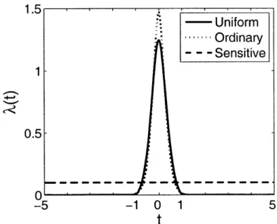
We compare the CS-optimized quantizer, called the "sensitive" quantizer, to a uni-form quantizer and "ordinary" quantizer which is optimized for the distribution of y through (2.10). The ordinary quantizer would be best if we want to minimize distor-tion between y and 9, and hence has a flat sensitivity curve over the support of y. The sensitive quantizer Ac,(t) is found using (3.5) and the uniform quantizer Auni(t) is constant and normalized to integrate to 1.

If we restrict ourselves to fixed-rate scalar quantizers, the high-resolution approxi-mation for quantization distortion (2.11) can be used. The distortion for an arbitrary quantizer Aq(t) with rate R is

D(R)

2-

2_RE _s(

1)

[12A2(yi)

=

2R Yc2s(t)fyi(t)dt _12A2( _dt.

(3.7)

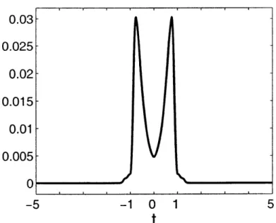
_(3.7)

Using 1000 Monte Carlo trials, we estimate ycs(t) in Figure 3-3. Note that the estimate is found through importance sampling since there is low probability of getting samples for large yi in Monte Carlo simulations. The sensitivity is symmetric and

(37)

0.03 0.025 0.02 0.015 0.01 0.005 0 -5 -1 0 1 5

t

Figure 3-3: Estimated sensitivity sy,(t) via Monte Carlo trials and importance sam-pling for (K, M, N) = (5, 71, 100).

peaks away from zero because of the structure in (3.3). Some intuition is provided in Appendix 3.C for the scalar case. The point density functions for the three quantizers are illustrated in Figure 3-4.

Experimental results are performed on a Matlab testbench. Practical quantizers are designed by extracting codewords from the cdf of the normalized point densities. In the approximation, the ith codeword is the point t such that

(t')dt' i - 1/2 X(t')dt' 2.R"

where Ri is the rate for each measurement. The partition points are then chosen to be the midpoints between codewords.

We compare the sensitive quantizer to uniform and ordinary quantizers using the parameters a2 = 0.3 and y = 0.1. Results are shown in Figure 3-5.

We find the sensitive quantizer performs best in experimental trials for this com-bination of a 2 _{and p at sufficiently high rates. This makes sense because As(t) is a}

high-resolution approximation and should not necessarily perform well at very low rates. Numerical comparisons between experimental data and the estimated

(38)

quanti-1.5

1

0.5

0

-5 -1

Figure 3-4: Estimated point density (K, M, N) = (5, 71, 100).

0 1

t

functions Acs,,(t), Aord(t), and Auni(t) for

-2 -4 .0 0 ---- Sensitive -8 ... Ordinary - - - Uniform -10 2 3 4

component

5 6

rate R.

Figure 3-5: Results for distortion-rate for the three quantizers with ac2 = 0.3 and P = .01. We see the sensitive quantizer has the least distortion.

(39)

zation distortion in (3.7) are similar.

3.A

Proof of Lemma 3.1

Consider a unit hypersphere of dimension M - 1 centered at origin in the space of RM". We draw N vectors Oj uniformly from the surface of the hypersphere and form a matrix 4 E RM x N_. _{VWe show that every entry of 4 is identically distributed and}

the cdf of each entry Wij is

1-T(v,M), 0<v<1; F, (v, M) = T(-v, M), -1 < v < 0; 0, otherwise, where (M p arccos(v) T(v, M) - 2M-1 (sin 0)M- 2 dO

and F(-) is the Gamma function.

Proof. We begin by noting that an (M - 1) hypersphere (in IR) with radius R has surface area

S(M, R) =

'

(3.8)

where F(.) is the Gamma function.

Because we are drawing uniformly over the shell, the fraction of the hypersphere in the region satisfying the constraint vi > v is Pr(vi > v). This is found through the integration

Pr(vi > v) ) S(M - 1, sin O)dO

S(M, 1)

J0

for v E [-1, 1].

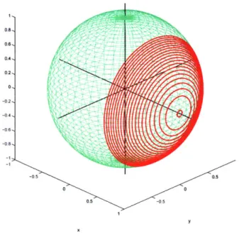
Geometrically, the integration is over every (M - 2) hypersphere in the region {v < vi _ 1} (or equivalently {arccos(v) > 0 > 0}). Figure 3-6 visualizes the integration for the case M = 3.

(40)

0.6.

0.2,

-0,2,

-0.5 0.5

0.5 -0

Figure 3-6: Integration over the circles that form the unit spherical shell for 0 < 0 < arccos(v).

We simplify the integral using (3.8):

Pr(vi > v) = F 2 ) arccos(v) M-1 (sin)M-2 2- 2 (si d) ]p(M 2 1 M- 1

JF(")

I

arccos(v) (sin O)M - 2dO a T(v, M).

By symmetry, Pr(vi > v) = Pr(vi < -v) and hence the cdf is

Fv (v, M) = Pr(vi < v) = 1 -T(v, M), T(-v, M), 0, 0<v<1; -1 <v < 0; o.w.

(41)

Since 4J is constructed from N independent v vectors, we can also use symmetry arguments to show every entry ij is identically distributed. We now make some remarks about the distribution of I4 ij:

1) Unfortunately, the distribution of bij is difficult to compute analytically (it is a sum of hypergeometric functions). Instead, one can use numerical methods to find both F, (v, M) and the probability density function (pdf) fv, (v, M).

2) The distribution is always symmetric around 0 and has a support of [-1, 1]. 3) As M increases, the distribution becomes more peaked around 0 and ap-proaches a Dirac delta.

4) Because every column vector must have unit norm, the entries in a column of 4 are not independent. However, since the columns are chosen independently, entries across rows are independent.

One can easily generate v by just creating a random Gaussian M x N matrix and then rescaling the columns to have unit norm. Figure 3-7 compares the results from this lemma (red line) with the empirical distribution (blue bars) formed through Monte Carlo trials for several values of M. We see the empirical results match the theoretical distribution very well.

3.B

Functional Quantization Example

We present a pedagogical fixed-rate scalar quantizer example to build intuition for functional quantization. Assume yl and Y2 are uniform random variables, iid 11(0, 1). They are quantized separately and we wish to minimize the distortion of the function

9(Y1, Y2) = Y12 + Y22

By (2.10), the best quantizer to minimize distortion for each yi is uniform. How-ever, it is clear that this is not the optimal choice for g(y1, Y2) since a small pertur-bation for larger yi leads to a larger distortion penalty in the function g.

(42)

M=2 x10~ 6 5 4 3 2 0 1 -1 -0.5 0 0.5 1 x10 ~ M=10 6. -0.5 0 114 0.5 1 4 3 2 1 6, -0.5 Figure 3-7: Theoretical validate Lemma 1.

versus empirical distribution for different values of M to

sensitivities are -yi(t) = 2t, meaning the optimal point density is

5 t2/3 3, 0,

t [0, 1];

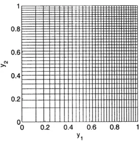
O.W. (3.9)

The quantization cells of this quantizer are visualized in Figure 3-8. As predicted, larger values of yi have higher resolution because those values have more weight in the distortion calculation.

Using (2.15), the resulting distortion of the sensitive quantizer is approximately

12 2R where R is the rate for each quantizer. This is better than the ordinary

quantizer (optimal for the observations), which leads to a distortion on g of 2 R

0.5 1

M=3

(43)

0.8

0.6

0.4

0.2

0 0.2 0.4 0.6 0.8 1

Figure 3-8: Quantization cells of a sensitive quantizer for the function g(y1, Y2) S2+y 12. The cells for larger values of yi are smaller and hence have better resolution.

3.C

Scalar Lasso Example

We consider a scalar version of the quantized compressed sensing problem. This example has little applicable purpose, but illuminates how the sensitive quantizer is shaped for lasso.

Assume we implement the system shown in Figure 3-9. The scalar random variable x is assumed to have the Laplacian pdf

fx

(; m, b) = 2b exp Ib

-Meanwhile, r is additive Gaussian noise and the reconstruction function g is the MAP estimator

= arg min (Ily - x112 + PIIxII1) (3.10)

that we call scalar lasso. Like lasso, it has a signal fidelity and sparsity tradeoff, with the regularization parameter p determined by the noise variance.

(44)

Figure 3-9: Model for scalar lasso example. Assume x is a compressible source and y = x + rt. The measurements are scalar quantized and then used to reconstruct Ri through scalar lasso.

Functionally, the reconstruction is

X + P, x < ~;

g(x) = 0, X < -L < x < ; (3.11)

X-- /j, X > P

The scalar lasso function k = g(x) is shown in Figure 3-10, along with the ordinary and sensitive quantizers. The ordinary scalar quantizer, where the point density is optimized for

f,(y),

is represented by the diamonds. Meanwhile, the sensitive quantizer also takes into account the sensitivity and is represented by the dots on the same plot (using don't-care regions as described in [50]). Similar to the results presented in the vector case (Section 3.5), the sensitive quantizer puts less weight near zero due to lasso shrinkage.

(45)

:.eeee 0 0 0

S-- Lasso

rule

+

Ordinary

* Sensitive

Figure 3-10: Scalar lasso and its quantizers. The functional form of lasso is repre-sented by the solid green line and demonstrates lasso shrinkage in that the output has less energy than the input. The ordinary quantizer is shown in the red diamonds and the sensitive quantizer is represented by the blue dots.

(46)

Compressive sensor networks : fundamental limits and algorithms

Compressive Sensor Networks:

Fundamental Limits and Algorithms

by

John Zheng Sun

B.S. Electrical and Computer Engineering, Cornell University (2007)

Submitted to the Department of Electrical Engineering and Computer

Science

in partial fulfillment of the requirements for the degree of

Master of Science in Electrical Engineering and Computer Science

at the

MASSACHUSETTS INSTITUTE OF TECHNOLOGY

September 2009

@

John Zheng Sun, MMIX. All rights reserved.

The author hereby grants to MIT permission to reproduce and

distribute publicly paper and electronic copies of this thesis document

in

whole

or in part.

TNSTITUTE

A

SEP 3 0 2009

LIBRARIES

A u th or

... ./ ... . ... ...

Department of Elctrical Engineering and Computer Science

i

ASeptember

2, 2009

Certified by

...

v1".

'

".. .

...

Vivek K Goyal

Esther and Harold E. Edgerton Associate Professor of Electrical

Engineering

Thesis Supervisor

A

ccepted by ... ,...

... ...

Terry P. Orlando

Chairman, Department Committee on Graduate Theses

Compressive Sensor Networks:

Fundamental Limits and Algorithms

by

John Zheng Sun

Abstract

Acknowledgments

Contents

List of Figures

Chapter 1

Introduction

1.1

A Peek at Compressed Sensing

1.2

Thesis Outline

Chapter 2

Background

2.1

Compressed Sensing

2.1.1

History

2.1.2

Incoherence and the Restricted Isometry Property

4j

2.1.3

Reconstruction Algorithms

(N)

(Ily

2.1.4

Extensions and Applications of

CS

e

2.2

Quantization

2.2.1

Optimal Quantization

_Q