Biometrika (1961), 48, 3 and 4, p. 419 4 1 9 Printed in Great Britain
Computing the distribution of quadratic forms in
normal variables
BY J. P. BfflOF
University of Geneva 1. INTHODUCTION
In this paper exact and approximate methods are given for computing the distribution of quadratic forms in normal variables. In statistical applications the interest centres in general, for a quadratic form Q and a given value x, around the probability P{Q > x). Methods of computation have previously been given e.g. by Box (1954), Gurland (1955) and by Grad & Solomon (1955). None of these methods is very easily applicable except, when it can be used, the finite series of Box. Furthermore, all the methods are valid only for quadratic forms in central variables. Situations occur where quadratic forms in non-central variables must be considered as well. Let x = (xlt ...,xn)' be a column random vector which follows a multidimensional normal law with mean vector O and covariance matrix Z. Let (i = (/*!, ...,/fn)' be a constant vector, and consider the quadratic form Q = (x + fi)'A(x + n).
If S is non-singular, one can by means of a non-singular linear transformation (Scheffe (1959), p. 418) express Q in the form m
Q= ZK&;£- (1-1) r - 1
The A,, are the distinct non-zero characteristic roots of AZ, the hr their respective orders of multiplicity, the 8T are certain linear combinations of /ilt ...,fin and the Xhr; a« are independent
^-variables with hr d.f. (degrees of freedom) and non-centrality parameter 6*. The variable
A
XHI* is defined here by t h e relation Xhi' — (xi + <?)3 + 2 *?. where xvx2, ...,xh are
inde-2
pendent unit normal deviates. In case Z is singular but A is not, a similar decomposition can be obtained except that an additive constant might figure in the right-hand member of (1 • 1). This is the case for instance if Q = (xx -I- x2)2 + x\, where the linear constraint xx + xt — c is imposed.
We illustrate the reduction of a quadratic form to the form (1-1) on the correlator
w =
I
where the xt and yi are normal deviates with zero means and we assume that cov (xt,Xj) = cov{yitj/y) = Si}, cov(xltjry) = pSi} and \p\ < 1.
Expressions for the probability density of w have been given in some particular cases of these assumptions by Roe & White (1961). Let
z= (x1,...,xn,y1,...,yn)' and $ = (f*i,—,fin>Vi
7»)'-Then w = (z — %)' A(z — £), where A and the covariance matrix Z of z can be partitioned into square submatrices of n rows each: If U denotes the unit (identity) matrix,
z = |
uu
Under the linear transformation z* = Pz, where
the correlator takes the form w = (z* — £*)' A*(z* — £*), where £* = P£ and A* is a diagonal matrix having its n first diagonal elements equal to p — 1, the n remaining ones equal to p + 1. The covariance matrix of z* is the unit matrix. The random variable w can therefore be written
a linear combination of two independent ^-variables with non-centrality parameters
S\ =
2. FINITE EXPRESSIONS
Box (1954) has considered the case where in (1-1) 8? = 0 and hr = 2yr(r = 1, ...,m), the t>r
being positive integers. In statistical applications, it is often possible to arrange for the d.f.'s to be even. A problem in the theory of Gaussian noise where this condition is always fulfilled is described by Davenport & Root (1958). Box has then expressed the probability
P{Q > x) by means of a finite series of x* probabilities. Using a different proof, a modified and
often more convenient form of his result will be obtained, as well as a corresponding expres-sion for the probability density g(x) of Q. Suppose Ax>..., A^ have been ordered, so that
m p
A1> Aa> . . . > Ap> 0 > A_+1 > ... > An,. Let n = ^vT and q = 2 >r.
I I THEOEEM. If x > 0, then
where Fk(\, x) = A""1 exp { - x/(2A)} fl (A - A,
l
r - l
r+k
Proof. Let AJ,..., A^, A ^ j , . . . ,A^ be real, pairwise unequal parameters such that A^ > 0 for
n
8= 1, ...,q and Ai < 0 for a = q+ 1, ...,n. Let Q' = YiKx\(8)> where the n ^-variables xi(«) I
with two d.f. each are independent. The characteristic function <f>'(t) of Q' is
1
and correspondingly the probability density is
The integrand having simple poles only, one finds for x > 0
Computing the distribution of quadratic forms in normal variables 421
in which X and Y are independent Poisson variables with expected values \x and ^J2,
respectively. Johnson (1959) rediscovered this equality and used it as a starting point to k The density g(x) of Q can now be obtained by a passage to the limit. Let a0 = 0, crk = 2 vr
r - l
for k = 1 ro. For positive distinct integers a, b, ...,d all not larger than m, denote by lim the passage to the limit
bd
Then g(x) = lim g'(x) can be written
1,2 m
p at at t - 1 * «-(r»_,+ l */-eri_,+l
x lim Yl (Ag —A^)"1 lim n I
1 k-l *<<n-i k+l m 4>n
P at
t - 1 k M-at-,+ 1
where/i(A, x) = (3/3x)i^(A, x). One recognizes the summation over a as the divided difference
of order vk— 1 of the function fk(A,x), corresponding to the vk 'abscissas' A^_1+1,..., A^t.
Hence, by a well-known result, one has for x > 0
(2-2)
Upon integrating this expression, formula (2-1) results. For x < 0, one must substitute S for - 2 in (2-2) and 1 - £ for £ in (2-1).
i I JJ+I l
A particular case of the theorem is
Even using this, it is not easily possible to establish in general the equivalence of (21) with formula (2-11) of Box (1954).
The formulae (2-1) and (2-2) are very convenient to use when all vk are small. With
in-creasing vks, the labour of computing the corresponding derivatives of Fk(\, x), or /t(A, x)
rapidly becomes considerable. The numerical method of the next section is then often easier to apply.
Consider now the case where the variables are non-central. The characteristic function of
( 1 1 ) i B 1
(2-3)
To obtain the probability density by integration of the inversion formula appears hopeless, except in the particular case m = 1. One finds then for the density pn(x, 8*) of ^n-t* the
Nation pJ 3t) k { U + Si)} ( i /» * » - i Ii n_l {S x i ) , (2-4)
where I,(z) is the Bessel function of purely imaginary argument, of order v. This formula has been given first by Fisher (1928) who pointed out on the same occasion the relation
derive some simple approximations for P{xii;j« < x}- However, expressions in finite terms
obtainable for such probabilities, when n is odd, by integrating (2-4) do not seem to have previously been written down explicitly. We shall give the first few of them, which are simple enough to be useful in numerical work. I t is necessary to assume n > 1. Write then n = 2m + 3 (m = 0,1,...). A classical formula permits the expression in finite terms of the Bessel function of half integral order appearing in (2-4). One finds
2 ( - lYA
m(r,x) + {- l ^ e - l *
1S AJr.x)],
r-0 r-0 Jwhere a= z* - 8, b = x^ + 8, Am(r, x) =
2 M ( m - r ) !
The above density can be integrated explicitly. If I(x) denotes the cumulative distribution function of a unit normal variable, the result is found to be
~-^[Kn(8,a)-Kn(8, -6)],
where Kn(8,x) = exp{ — \x2}Pn(8,x) and Pn(8,x) is a polynomial in 8 of degree n—3. The
general expression for Pn(8, x) is not simple. The polynomials corresponding to the values
n = 3,5, 7 and 9 are
Pz(8, x) = 1, Pb(8, x) = 28* + x8 - 1, P7(8,x) = 38i + 3x33+(x2-4:)82-3x8+3,
P9{8,x) = 4<J6+6x^8+(4x2-10)(J4 + (x3-15a;)53-(6xi i-18) 8i+ 15x8- 15.
In the applications, b is often large enough so that one can assume I(b) = 1, Kn(8, —b) = 0.
3. NUMERICAL INVERSION OF THE CHARACTERISTIC FUNCTION
In this section we show that the cumulative distribution function F(x) of the variable Q defined by (11) can be obtained quite easily by straightforward numerical integration of an inversion formula. The standard inversion formula gives an expression not for F(x) itself, but for the difference F(x) —F(0). If Q, as is the case, for instance, in (1-2), is not strictly positive, a formula is needed which gives F(x) directly. Such a formula is implicit in work of Gurland (1948) and has been later derived explicitly by Gil-Pelaez (1951), namely
F(x) = i - ^
where f{z) denotes the imaginary part of z and where the characteristic function <f>(t) of
Q is given by (2-3). Using the relations
arg[(l-t&0~"] = ff tan-1 (it), \(\-ibt)-o\ = (1 + bHs)-l<>,
arg[exp{ia</(l-t&0}] =
one finds that for the quadratic form Q of (11), equation (3-1) can be written, after the substitution 2t = u is made,
Computing the distribution of quadratic forms in normal variables 423
1
d(u) = l- S [hr tan-i (A^) + *? Ar«( 1 + AJu')"1] - £xu, ^ I
n
The following relations are immediate
— oo if x > 0,
<?(«) = | +0 0 if * < 0 ,
The function up(u) increases monotonically towards + oo. Therefore, in numerical work the integration in (3-2) will be carried over a finite range 0 < u < U only; the degree of approxi-mation obtained will depend (apart from rounding-off errors) on two sources of error: (i) the ' error of integration' resulting from the use of an approximate rule for computing
ru
Iv = 7T-1 [upiu)]-1 sin d(u) du, Jo
and (ii) the 'error of truncation'
tv = TT1 \up(v)Y1sxn.d(u)du.
Ju
Noticing that x > y implies xi(l+xi)~1 > j/*(l +yi)~1, one finds that \tv\ can be bounded above by Tv, where
1 m
and where we have put k = - 2 hT. One can hopefully expect that Tv will often be
satis-2 I
factorily small, even for moderate values of U. It does not seem feasible on the other hand to obtain an upper bound for the error of integration resulting from the application of a standard quadrature formula. With equal step formulae (in the application of which the ordinate at the origin is given by (3-3)), a common procedure is then to carry out the integra-tion repeatedly, each time halving the step of integraintegra-tion until two consecutive results agree to the desired accuracy. In order to gather some more detailed information relative to the performance of the two simplest and most commonly used rules, namely, the trapezoidal rule and Simpson's rule, we have preferred to follow a different procedure. Given a tolerance e, numerical integration in (3-2) was carried out by using steps of length j/10. The integer j was then increased, one unit at a time, until the largest value was attained such that, for the first even number of steps yielding a bound Tv < e, the values of the integral obtained by the trapezoidal rule and by Simpson's rule, say JT and Js, still satisfy \JT — Ja\ < e- Results for the values e = 0-01 and e = 0001 are given in Table 1. The following unexpected behaviour was observed in all cases: As j increases, Js departs from the correct value of the integral' more rapidly' than does JT. In other words, to achieve a given accuracy, longer steps are per-missible with the trapezoidal rule than with Simpson's rule. Some computations made with
424
J. P. IMHOFa formula (sometimes referred to as Hardy's rule) based on approximation of the integrand with polynomials of degree six seem to indicate that in fact, the higher the degree of the approximation polynomials used, the shorter the step of integration must be. Accordingly, only the results obtained with the trapezoidal rule are recorded in columns (i) and (ii) of Table 1 and are seen to be of much greater accuracy than the value of e would let one
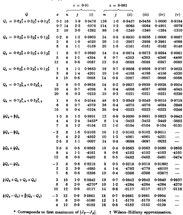
Table 1. Probability that the quadratic form Q exceeds x
(i) Integration in (3-3) with the trapezoidal rule and n steps of length j , for tolerance e = 0-01; (ii) same for tolerance e = 0-001; (iii) exact values; (iv) Pearson's three-moment %* approximation; (v) Patnaik's two-moment %* approximation.
e = 001 e = 0-001 Q Qi = <3i = o6*J + 03*5 -Qt = 0-6*! + 0-3*1 + 0-1*5 Q* = 0-6*J +0-3*1+ 0-l*J <2, = 0-7*;.,+0-3*;., 0 . =
40. + W.
W.-W.
X 0-1 0-7 2 0-2 2 6 1 5 12 1 3 8 2 10 20 1 6 15 1-5 4 7 - 2 0 2-6 3-6 8 13 - 2 2 7 3 6 10 - 3 0 4 n 16 14 10 8 6 8 6 4 8 8 6 10 6 4 6 8 6 8 8 4 8 6 4 8 6 4 6 6 2 6 10 6 12 12 6 12 j 1-9 2-2 3 0 1-2 1-9 1 1 0-7 1 1 0-6 11 1-4 0-8 0-3 0-7 0-3 0-4 0-7 0-4 1-2 2-4 1-2 1-6 2-2 11 0-6 11 0-6 0-6 3-9 0-6 10 2 0 0-9 0-9 2 0 0-9 (i) 0-9478 •5076 •1262 0-9903 •4020 •0159 0<9980 •4354 •0087 0-9663 •4201 •0088 0-9938 •4098 •0223 0-9544 •4079 •0224 0-9891 •3463* •0154 0-9103 •4052 •0097 0-9563 •4161 •0462 0-9218 •4685 •0396 0-9842 •4270* •0117 0-9861 •5180 •0162 n 136 114 86 24 20 20 14 8 12 16 10 14 14 8 10 48 36 36 12 8 12 10 10 14 10 8 8 8 4 10 16 10 14 18 12 16 j 1 0 1-2 1-6 0-8 1 0 1 0 0-4 0-7 0-5 0-7 1 0 0-8 0-2 0-4 0-3 0-3 0-4 0-4 0-9 1-4 1 0 1-2 1-3 0-8 0-4 0-6 0-5 0-5 1-4 0-4 0-7 1-2 0-8 0-7 1 1 0-8 (ii) 0-9457 -5066 •1240 0-9930 •3997 •0161 0-9974 •4353 •0088 0-9666 •4195 •0087 0-9937 •4086 •0221 0-9549 •4076 •0223 0-9890 •3453 •0164 0-9102 •4061 •00fl8 0-9563 •4162 •0462 0-9218 •4782 •0396 0-9842 •4264 •0117 0-9861 •6170 •0152 (iii) 0-9458 •6064 •1240 0-9936 -3998 •0161 0-9973 •4363 •0088 0-9666 •4196 •0087 0-9939 •4087 •0221 0-9649 •4076 •0223 0-9891 •3453 •0154 0-9102 •4061 •0097 0-9563 •4152 •0462 0-9218 •4779 •0396 0-9842 •4264 •0117 0-9861 •6170 •0152 (iv) 10000 0-4901 •1264 10000 0-3961 •0162 0-9984 •4346 •0087 0-9767 •4156 •0086 0-9928 •4089 •0221 0-9515 •4084 •0223 0-9923 •3449 0154 0-9011 •4221 •0032 0-9560 •4163 •0461 0-91661 •4810f •0387t 0-9840 •4264 •0117 0-9904 •5164 •0139 (v) 0-9184 •5079 •1310 0-9867 •4098 •0145 0-9961 •4400 •0080 0-9522 •4330 •0066 0-9954 •4045 •0230 0-9719 •3948 •0246 0-9842 •3552 •0131 0-9605 •4101 •0474 0-9837 •4270 •0116 —,-«.) + *<«.-«.)
Computing the distribution of quadratic forms in normal variables 425
suspect. We have in several cases computed the correction terms, up to the one involving finite differences of orders one to six, which are to be added to the trapezoidal rule according to Gregory's formula. They have proved to give no reliable estimate of the error of integration resulting from the use of the trapezoidal rule. For e «= 0-01, it was found in two cases that
&sj increases, \JT — Js\ first increases to reach a maximum smaller than 0-01, then decreases
again. The results corresponding to the value of j for which | JT — J81 attains its first maximum
are then recorded. It is clear that under such circumstances, the procedure we have followed is not an adequate one to use in general practice. Another example of this is provided by
Q = $Q6 — %Qe, for x = 2. In this case, it was necessary to increase,; up to 3-9 before \JT — Ja\
reached e = 0-01, while two steps of length 1-5 already make Tv < 0-01 and give the better
value 0-4787. I t is hoped, however, that a sufficient variety of quadratic forms is covered so that Table 1 can serve as a useful guide for the length of the step of integration to be used in
m
any particular case. To help in this purpose, all quadratic forms listed satisfy 2 I'M = 1-The probability density g(x) of the quadratic form Q could be computed by using a formula analogous to (3-2). In fact,
g(x) = 7T-1 f l X t O ^ c o s t f M d t t . JO
Due to the absence of the factor u- 1 in the integrand, numerical integration, for the same
accuracy, can be expected to require a slightly larger number of steps than is needed to compute the distribution function.
4. T H E ACCURACY OF SOME APPBOXIMATIONS
Recently Johnson (1959) has shown that Pearson's (1959) three-moment central #• approximation to the distribution of non-central ^* is remarkably accurate in both tails of the distribution. I t is therefore natural to extend this approximation to the general case of the quadratic form Q of (1-1). Let E(Q) and <r(Q) be the mean and standard deviation of Q. Following Pearson, we write for a positive quadratic form Q,
Q Z (£'-h')(2h')-i(T(Q)+E(Q),
and determine h' so that both members have equal third moments. This amounts to taking
P{Q * x) = P{£. > y), (4-1)
where A' = ct/c|, y = (x-cj (h'fa*+ h', c, = piiK+3^) 0=1,2,3).
If Q is non-positive, the same approximation can be used but one must assume that c, > 0. Otherwise, approximate the distribution of — Q. The values obtained from (4-1) are shown in column (iv) of Table 1. For the quadratic form ±Q5 — ^Qs, one has h' = 1395-85. In this
case, the Wilson-Hilferty approximation was used to evaluate the right-hand member of (4-1). The merits of the three-moment approximation are obvious, particularly in the upper tail of positive quadratic forms. For such forms, the approximate values given by the standard two-moment (Patnaik) approximation are indicated in column (v). I t is seen that the three-moment approximation, which requires very little more work, gives a much better fit than is achieved with the Patnaik approximation. While there is an appreciable loss of accuracy for non-positive forms, the approximation still gives useful indications which can suffice for certain practical purposes.
Most of the computations summarized in Table 1 have been performed on the Ferranti ' Mercury' computer at CERN, Geneva. I am much indebted to the late Director General of that organization, Prof. C. J. Bakker, who made it possible for me to use the faculties of the computer service.
I wish to thank the Referee for suggesting some notable improvements in the presentation of the paper.
REFEBENCES
Box, Q. E. P. (1954). Some theorems on quadratic forms applied in the study of analysis of variance problems, I. Effect of inequality of variance in the one-way classification. Ann. Math. Statist. 25, 290-302.
DAVBNPOBT, W. B . <fe ROOT, W. L. (1958). An Introduction to the Theory of Random Signals and Noise. New York: McGraw-Hill.
FISHEB, R. A. (1928). The general sampling distribution of the multiple correlation coefficient. Proc. Roy. Soc. A, 121, 664-73.
GIL-PKLAEZ, J. (1951). Note on the inversion theorem. Biometrika, 38, 481-2.
GRAD, A. & SOLOMON, H. (1955). Distribution of quadratic forms and some applications. Ann. Math. Statist. 26, 464-77.
GURLAND, J. (1948). Inversion formulae for the distribution of ratios. Ann. Math. Statist. 19, 228—37. GUKLAND, J. (1965). Distribution of definite and indefinite quadratic forms. Ann. Math. Statist. 26,
122-7.
JOHNSON, N. L. (1969). On an extension of the connexion between Poisson and %* distributions. Biometrika, 46, 352-63.
PEABSON, E. S. (1959). Note on an approximation to the distribution of non-central %*• Biometrika, 46, 364.
ROE, G. M. & WHITE, G. M. (1961). Probability density functions for correlators with noisy reference signals. IRE Trans, on Information Theory, IT-7, 13-18.