Commercial real estate volatility : a decomposition of historical market values

(1)

Commercial Real Estate Volatility: A Decomposition of Historical Market Values by

Christopher J. Whittier B.A., Economics, 2011 The Johns Hopkins University

Submitted to the Program in Real Estate Development in Conjunction with the Center for Real Estate in Partial Fulfillment of the Requirements for the Degree of Master of Science in Real Estate Development

at the

Massachusetts Institute of Technology September, 2019

The author hereby grants to MIT permission to reproduce and to distribute publicly paper and electronic copies of this thesis document in whole or in part in any medium now known or hereafter created.

Signature of Author_________________________________________________________ Center for Real Estate

July 26, 2019

Certified by_______________________________________________________________ William Wheaton

Professor, Center for Real Estate

Professor Emeritus, Department of Economics Thesis Supervisor

Accepted by______________________________________________________________ Professor Dennis Frenchman

Class of 1922 Professor of Urban Design and Planning, Director, Center for Real Estate

(2)

2

Commercial Real Estate Volatility: A Decomposition of Historical Market Values

by

Christopher J. Whittier

Submitted to the Program in Real Estate Development in Conjunction with the Center for Real Estate on July 26, 2019 in Partial Fulfillment of the Requirements for the Degree of Master of Science in Real Estate

Development

ABSTRACT

Risk—both its mitigation and its exploitation in pursuit of profits—is likely the most important topic in the study of investment. Risk in private market commercial real estate, however, has been historically less well understood than other more liquid asset classes. To date, most of the research on risk in real estate investment has focused on how

changes, cycles, or shocks in the underlying space or asset markets occur. This paper furthers the study of commercial real estate risk by decomposing historical asset volatility into its component space and asset market parts. We do this through the application of a variance decomposition framework on NCREIF NPI time-series data

that has been detrended of long-term secular market movements. In doing so, we are able to compare the relative contributions of space and asset market volatility to commercial real estate price volatility and, more importantly,

demonstrate how the expectations of investors who sit at the intersection of those two markets may play an overlooked role in moderating or augmenting volatility.

Thesis Supervisor: William Wheaton Title: Professor, Center for Real Estate

(3)

3

I. Introduction

Risk—both its mitigation and its exploitation in pursuit of abnormal profits—is likely the most important topic in the study of investment. In traditional investment markets, such as those for publicly traded stocks and bonds, risk has been studied rigorously and is a concept well understood by even novice investors. Real estate, by contrast, is an asset class where risk has been historically less well understood and remains a somewhat opaque concept to most investors. The relative illiquidity of private market real estate as well as well as the dearth of transparent, consistent, and widely available historical real estate investment data have been significant drivers of this issue. Additionally, lack of risk management tools such as the ability to sell short or hedge real estate investments, as well as the difficulty for all but the most sophisticated institutional investors to truly diversify their real estate holdings, may have also limited the practicality of such study in the past (Ling, Naranjo, Scheick (2014)). Recently, however, the proliferation of better sources of

commercial real estate data has enabled a relatively small group of land and financial economists to adapt methodologies originally developed for publicly traded asset classes to the field of real estate, furthering our understanding of risk.

Investment grade real estate, like other financial assets, generates economic value through the cash flow that it provides and the change in value it experiences over time. Variations in the cash flow component are driven by changes in property rents and expenses that reflect conditions in the space market, while variations in real estate values or prices represent changing conditions in the asset or capital markets. Together, the returns generated from each of these components constitute the total return of a real estate asset. The variance or standard deviation of total returns is used to quantify ex post risk in real estate assets.

To date, most of the research on risk in real estate investment has focused on how changes, cycles, or shocks in the underlying space or asset markets affect their respective total return components over time. Generally, that research suggests that asset value volatility is responsible for a greater share of total variation over time. The NCREIF National Property Index (NPI), a total return index intended to measure the performance of a portfolio of institutionally held private market real estate investments, seems to confirm that research. Over a thirty-year horizon, valuations have accounted for more than 95% of total return volatility across all major property types. Yet, this simplified analysis, as well as others conducted on commercial real estate return volatility, is somewhat

(5)

5 misleading because it does not fully describe the ways that space and asset markets effect volatility. While the income component can be parsed out explicitly, as it is in the NCREIF NPI data, this represents only the changes in an investor’s total return due specifically to income—often referred to as current yield. We also know that income is a fundamental determinate of a property’s current value, which we can see from two common valuation methodologies. The first, the discounted cash flow (DCF) methodology, relates a property’s value to its future cash flows, discounted at an appropriate opportunity cost of capital (rt).

(1) DCF = ∑

( )

The second, the direct capitalization method, defines a property’s value as its current Net Operating Income (NOIt) income divided by an appropriate capitalization (“cap”) rate (Ct).

(2) V =

In both cases, the income of the property is joined with what we will refer to broadly as an asset or capital market assumption. In the DCF, this is the opportunity cost of capital. In the direct

capitalization method, the asset market assumption is given by the cap rate, also sometimes referred to as the ‘rent-price ratio.’ While we commonly describe the cap rate and OCC as asset market assumptions, the name is misleading because both rates also contain embedded assumptions about the space market. Put differently, both the cap rate and the opportunity cost of capital reflect capital market assumptions relative to the income risk profile of a specific asset.

For this reason, we believe that previous study of commercial real estate volatility, which has typically focused exclusively on either the space market or the asset market, has fallen short of fully attributing realized investment risk. Specifically, we hope to further decompose and quantify the relative contributions of income volatility and cap rate volatility to prices, while also exploring how the contemporaneous changes in space and asset market can exacerbate or limit price risk.

The rest of this paper will proceed as follows. We will next quickly review related literature on commercial real estate risk as well as the paper that inspired the analytical framework we have employed. In “Methodology’ we will introduce the decomposition framework and describe its application to commercial real estate prices, income, and cap rates. In “Data” we will discuss the key characteristics and considerations of the NCREIF NPI dataset as well as describe several data transformations that we have made to the underlying data. Variance decomposition results will be

(6)

6 presented in the “Empirical Analysis” section in addition to some broad discussion about our

findings in the context of the wider commercial real estate market. We will then conclude with a brief summary of our most significant findings.

II. Literature Review

Much of the preceding literature on the subject of commercial real estate market volatility has been focused on studying explicit drivers in the space or asset markets—effectively choosing to focus on one market exclusively. For instance, there is a body of work that has evolved our understanding of how real estate cycles are created by space market supply-demand dynamics. For instance, Grenadier (1995) explored how national and city-specific factors can explain variance office market vacancies, and subsequently how uncertainty in space market demand, coupled with the lagged nature of construction starts, can lead to boom-bust oscillations (1995). Wheaton (2015) provides a holistic view of the volatility of commercial space markets by explicitly apportioning the supply and demand side shares, and in doing so, shows that somewhat counterintuitively, well-coordinated supply can actually help to lower vacancy volatility.

On the other side of the valuation equation, many papers have been published on how broad asset market dynamics such as falling interest rates have influenced commercial real estate valuations [Conner and Liang (2004)]. Additionally, Duca, Hendershott, and Ling have demonstrated how changing tax policy over the past four decades has affected investors’ required returns, thereby generated price swings in CRE values. Clayton, Ling, and Naranjo (2008) further explored the relative role that investor sentiment, as opposed to asset market fundamentals, plays in commercial property pricing and return generation. In the wake of the global financial crisis, institutional interest real estate has expanded significantly given the persistence of a low interest rate environment. Fisher, Ling and Naranjo (2009) have found evidence that the institutional capital flows associated with heightened interest in private market real estate have positively impacted price appreciation and therefore subsequent total returns.

A relatively smaller body of work has been completed examining private market commercial real estate price volatility holistically. Much of the early work in regarding risk focused on securitized or public market real estate (REITS) due to the limited availability of private market real estate data. Chan, Hendershott, and Sanders (1990) first explored the composition of equity REIT returns and pricing. This work, which utilized Arbitrage Pricing Theory (APT) and the CAPM, still attempted to

(7)

7 relate risk to a series of macroeconomic and capital market ‘factors’ rather than to directly quantify the impact of changes in space and asset market fundamentals. The work that most closely

resembles the analysis presented in this paper is that of a series of papers which sought to

decompose private market real estate returns into expected and unexpected components. Liu and Mei (1994) used a VAR modelling process to predict and apportion historical REIT total returns, which Geltner and Mei (1995) then applied to private market real estate data (NCREIF). In doing so, Geltner and Mei were able to show that changes in expected future returns, as opposed to changes in expected cash flows, may actually drive most price volatility. While we find this research

innovative and academically rigorous, we believe that the particular present value framework

selected (cash flow forecasting and time-varying discount rates) is somewhat challenging in regard to practical interpretation. Additionally, as we have explained in the introduction, by simply dividing volatility into space and asset market drivers, this research stops short of examining how space market dynamics may in fact influence contemporaneous changes in asset market assumptions. Finally, it is worth noting that the premise and inspiration for this paper is largely based on the work of Wheaton (2015) in describing real estate vacancy volatility. We found his direct application of the variance decomposition process to vacancy data yielded a highly intuitive, and therefore powerful, explanation of the interaction between supply and demand drivers in overall space market volatility. We hope to replicate that process for commercial real estate prices.

III. Methodology

Variance Decomposition

To understand the relative contributions of income and asset market volatility to commercial real estate price volatility, we will be using a simple stochastic framework known as variance

decomposition. Variance decomposition relies on the fact that for any two random variables X and Y, the variance of the sum of those two variables is equal to the sum of the variances plus two times the covariance.

(3) 𝐯𝐚𝐫(𝐱 + 𝐲) = 𝐯𝐚𝐫(𝐱) + 𝐯𝐚𝐫(𝐲) + 𝟐𝐜𝐨𝐯𝐚𝐫(𝐱, 𝐲)

As demonstrated by Wheaton (2015) with commercial real estate vacancy rates, this relatively straight forward identity, which requires no advanced econometrics, can be applied to real estate data to measure and attribute risk. To implement the variance decomposition, we begin with the direct capitalization method for valuation previously described.

(8)

8

(4) 𝒗𝒕 =

𝒊𝒕

𝒄𝒕

We have chosen this valuation identity for its simplicity and measurability. The direct capitalization method is widely used by real estate practitioners and quantifies real estate values in terms of income (it), typically measured by NOI, and cap rates (ct). Not only are both variables easily understood but they are also easily observed in the market. By contrast, the DCF methodology requires a future cash flow forecast and an estimated discount rate—both of which are subjective and not widely collected. Unfortunately, the direct capitalization expression for the market value of real estate is not linear for its original parameters—a requirement to be decomposed via expression (3). We can, however, rewrite the valuation expression using a log-linear transformation that sets the log of the property value equal to the difference between the log of income (it) and log of the cap rates (ct).

(5) 𝐥𝐨𝐠(𝒗𝒕) = 𝐥𝐨𝐠(𝒊𝒕) − 𝐥𝐨𝐠(𝒄𝒕)

The log-linear expression (5) can now be combined with expression (3) to arrive at expression (6). The resulting identity is the basis for our variance decomposition.

(6) 𝐯𝐚𝐫[𝐥𝐧(𝒗_𝒕)] = 𝐯𝐚𝐫 𝐥𝐧(𝒊𝒕) + 𝐯𝐚𝐫 𝐥𝐧(𝒄𝒕) − 𝟐 ∗ 𝐂𝐨𝐯(𝐥𝐧(𝒊𝒕), 𝐋𝐧(𝒄𝒕))

Interpretation of Variance Decomposition Parameters

With this identity, it is now possible to exactly decompose valuation volatility into three distinct components: the share due to variance in income, the share due directly to variance in cap rates, and the share due to the covariance between variance in cap rates and variance in income.

For the purposes of this analysis we have chosen to interpret the variables that comprise expression (6) in a particular manner. Specifically, we will assume that income, which will be represented by NOI, is entirely a reflection of conditions in the space market and is therefore an exogenous variable. Cap rates on the other hand, we assume to be at least partially endogenous to our analysis. As we have noted, there is significant literature that demonstrates the relationship between cap rates and broader capital markets drivers such as prevailing interest rates, capital flows, and taxation policy.We also know, however, that cap rates reflect investor’s forward-looking assumptions about the growth or decline of rents in the space market, and reflect investor’s perception of the riskiness of a property’s cash flows relative to other properties or assets. Implicitly, in forming these forward-looking assumptions about growth and risk, investors must incorporate current information from the space market by considering current rent levels and, given space market supply-demand drivers,

(9)

9 how likely those levels are to persist or change. The extent to which each side of the market—asset and space—influence cap rates likely varies from property to property and even for the same

property throughout time. At this point in our analysis, we will simply acknowledge that observation of the space market, as reflected in current rent levels, influences investors’ valuations, which is then reflected in current cap rates.

Consideration of the information flow from the space market to the asset market that must occur in the valuation process leads us to the final term in our decomposition expression (6). Review of this expression demonstrates a simple, albeit not readily intuitive, concept that occurs as a result of the interaction between income and cap rates. Specifically, that valuations are affected not only directly by changes in income and changes in cap rates, but are also additionally affected by the

co-movement of those two variables. Mathematically, the effect of the covariance term on valuation volatility is straight-forward. If income and cap rates tend to move together, reflected by a positive covariance in our expression, the third term remains negative and counteracts or dampens the impact of cap rate or income change on valuations, reducing price volatility. If income and cap rates tend to move in opposite directions, reflected by a negative covariance in our expression, the third term assumes a positive value, increasing the impact of cap rate or income changes and overall volatility.

Given our interpretation of cap rates, which reflect expectations about the relative value of the property given current information in the space market, we will assume that the covariance between cap rates and income results from investors’ valuation process. Put differently, we assume that investors observe changes in property level income and alter their appraisals or offer prices accordingly. The covariance then can be interpreted in a very specific manner. As an academic matter, real estate market values and income levels, in real terms, are generally thought to be mean reverting—any increase or decrease will eventually, as a result of market forces, return to a ‘normal’ level. If investors truly believe in mean reversion, we should expect to see a positive covariance between income and cap rates reflected in stable valuations. For example, if investors believe that a change in income levels reflects a temporary deviation from normalized levels that will eventually revert, they should temper the impact of that change on their valuation, resulting in a corresponding movement in the cap rate. In that manner, we will interpret positive covariance between income and cap rates as investors pricing mean reversion into their valuations. This dynamic should lead to lower overall volatility in market values.

(10)

10 Conversely, if investors do not believe in mean reversion, and instead believe that changes in the space market will continue over the near term, we should expect to see a negative covariance between cap rates and income. This extrapolation can be viewed as the relative optimism or pessimism of investors. In the event that investors believe a current rent increase signals future growth, their valuation will not only reflect higher current rent, but also the greater value of the property today attributable to future rent growth. This outlook would be reflected in a lower cap rate and a positive covariance between cap rates and income. Alternatively, if investors believe that a rent decrease signals future declines in space market conditions, they will discount their current valuations to reflect that expectation, leading to cap rate expansion. If this behavior is persistent over time, we expect that overall market value volatility will be increased.

Because we have chosen to interpret cap rates as an endogenous variable being influenced by

observed changes in income, we should consider the covariance term and the cap rate term together. It is the combination or net result of these terms that truly reflects the impact of cap rate

fluctuations on valuations. Income, which we have chosen to treat as an exogenous fundamental variable, will be treated as a standalone component in the context of the variance decomposition expression.

𝐯𝐚𝐫[𝐥𝐧(𝒗𝒕)] = 𝐯𝐚𝐫 𝐥𝐧(𝒊𝒕) + 𝐯𝐚𝐫 𝐥𝐧(𝒄𝒕) − 𝟐 ∗ 𝐂𝐨𝐯(𝐥𝐧(𝒊𝒕), 𝐋𝐧(𝒄𝒕))

= 𝑠ℎ𝑎𝑟𝑒 𝑓𝑟𝑜𝑚 𝑖𝑛𝑐𝑜𝑚𝑒 + 𝑠ℎ𝑎𝑟𝑒 𝑓𝑟𝑜𝑚 𝑐𝑎𝑝 𝑟𝑎𝑡𝑒𝑠

Application of Variance Decomposition to NCREIF Data

Having established this interpretation of the variance decomposition expression, we can now perform a more thorough risk attribution analysis and capture the interaction between income and cap rates. In doing so, we may be able to observe how investors’ perception of particular asset classes or geography can exacerbate or limit volatility in commercial real estate prices.

In pursuit of that cause, we have conducted two separate analyses. In the first analysis, we will decompose the variance in commercial real estate values by the major property types included in the NCREIF National Property Index (NPI). Our aim is to compare differences between property types in overall magnitude of price volatility, the relative contributions to overall volatility from income and cap rates, and in the correlations between cap rates and income.

The NPI is comprised of five major property types: multifamily, office, industrial, retail and hotel. Additional granularity is available to further parse the NPI data, however, we have opted against

(11)

11 using that additional granularity due to the relatively small sample sizes of sub-property type

classifications. The start date for part one of this analysis was chosen so that an accurate comparison could be made across the five property types. In 1989, all of the property types have at least 100 assets with the exception of hotel, which even in 2018 has only 77 properties included in the index (Table IV).

In the second part of the analysis, we will conduct the same decomposition on a subset of the property types to observe any differences between locations within those property types. Of the five major property types included in the NPI, we have chosen to conduct this additional analysis on both the office and multifamily property types. Office and multifamily were chosen given their long history of inclusion in the index.

The geographic locations utilized in this part of the analysis are delineated according to Core-Based Statistical Areas (CBSAs). The CBSAs that we have included were chosen formulaically based on the relative size and length of their historical data series. Specifically, we included those CBSAs that had, on average, the largest sample sizes between the years of 2000 and 2018. The CBSAs chosen for the office analysis and the multifamily analysis are quite similar, with the exception of Houston and Phoenix that appear in the multifamily analysis but not the office analysis, and San Francisco and Anaheim, which appear in the office analysis but not the multifamily analysis. Importantly, while these MSAs were chosen in a simple formulaic manner, we feel that they represent a reasonable cross-section of the major commercial property investment markets, as well as, the major metro areas by population across the United States.

To ensure a significant sample size across all CBSAs, we have begun the analysis in 2000, generating 19 observations for each variable in each chosen location. For the office analysis, each CBSA has at least 20 properties by the start of 2000. For the multifamily analysis, each CBSA has at least 10 properties included in the index, with the exception of Los Angeles which only has 7 properties as of 2000. While this is admittedly a small sample size, Los Angeles represents a key commercial real estate market we would like to include. Additionally, while small at the beginning of the analysis, the number of LA properties included in the index quickly grows, reaching 100 properties as of year-end 2018 (Table V).

Before presenting the results of the two analyses, it is necessary to first discuss the NCREIF NPI data set that we have employed as well as several of the data transformations we completed to fit the data to our variance decomposition framework.

(12)

12

IV. Data

NCREIF NPI Overview

As has been noted, this paper has been constructed using the National Council of Real Estate Investment Fiduciaries (NCREIF) Property Index (NPI). The NCREIF NPI is a total return index intended to measure the performance of a portfolio of institutionally held private market real estate investments. The index was originated by a consortium of institutional investors, mostly pension funds, in conjunction with pension consultancy Frank Russell Company in an effort to establish a benchmark for private market real estate investments. Over the course of its history, the NCREIF NPI has become an integral tool for institutional investors to measure and evaluate risk, and now serves as a benchmark for several commercial real estate derivatives and exchange traded products. The NCREIF data begins in 1978 for all property types, with the exception of hotels, which begins in 1982. The index’s long historical time-series is desirable because it allows us to conduct our analysis through several real estate cycles.Additionally, as additional data providers have been added, the historical property and return information from their respective assets has been backfilled into the index, creating a more mature time-series representative of a wider range of properties. When a property is added, strict inclusion criteria ensure that the index reflects institutional quality assets under normal operating parameters1_{. As of Q4 2018, the index constitutes ~$611bn of private} market real estate assets.

In addition to both the quality and length of NPI data, our decision to use to NCREIF was motived by the fact that NCREIF reports additional datapoints that are not readily available in other

commercial real estate data sources. For instance, while RCA publishes a number of transaction-based commercial property indices, property level financial information is typically either not available or is estimated based on unverified sources. By contrast, NCREIF collects a series of property level metrics like Net Operating Income (NOI), CapEx, as well as appraised and transaction values, which are then used to calculate the index. The availability of aggregate, or ‘portfolio’ data is required for this analysis because, as will be explained in greater detail below, the NCREIF NPI is intended to measure the returns generated by private market commercial real estate

1_{For a full list of inclusion criteria, please see Frequently Asked Questions about NCREIF and the NCREIF Property Index} (NPI)

(13)

13 investments. While closely related, our analysis is intended to analyze changes in the levels of market values, income, and cap rates rather than the returns associated with changes in those values.

Data Caveats & Criticisms

While the NCREIF NPI is widely utilized and well-respected benchmark, it is, like all data sources, subject to a number of caveats that should be quickly outlined.

Constituent Property Mix: As previously noted, NCREIF's data partners are mostly large tax-exempt institutional investors (pension funds, foundations, endowments or their appointed investment advisors). As a result, there is likely a bias in the portfolio of properties included in the index. Pension funds are relatively risk averse investors that typically seek out stabilized assets in well established markets. These 'core' investments are intended to generate income to match long-term liabilities while minimizing material downside risk. Therefore, while diversified by property type and geography, the NPI is likely indicative of mostly high quality, low risk commercial real estate assets. Evidence of this bias towards high-quality core assets is reflected in the NCREIF cap rates, which are significantly below the current national averages across all property types (Table II).

Index-Construction: As opposed to a repeat-sale index methodology, which controls for the underlying differences in properties by comparing the sales of the same properties across time, the NPI is dynamic in nature. A number of properties are introduced each quarter as member

organizations make new investments, and similarly, properties are removed from the index as they are sold. Therefore, over the time since its inception, both the size and the composition of the index have changed (Figure I). Review of the geographic composition of the index (Figure II) shows that most property types have either remained, or become slightly more, geographically diversified. The exception appears to be the office market, which has become more concentrated in the western and eastern regions of the US—likely a result of investors’ preference for assets located in resilient ‘gateway’ markets like New York, Boston, San Francisco and LA.

In addition to being a dynamic index, the NCREIF NPI is also considered an ‘appraisal-based’ index. Such an index, which relies on off-market valuations, is a response to the general illiquidity of commercial real estate. While including realized transaction prices in the index, NCRIEF largely relies on data providers’ own valuations of their properties. Therefore, as an appraisal-based index, the NPI could be affected by two key issues.

(14)

14 Self-reporting bias: Any data that is self-reported can potentially be subject to embedded bias or manipulation. NCREIF obtains its data from institutional investors who are not required, at least by NCREIF, to obtain third party verification of their valuations. With that being said, as fiduciaries to their clients and plan members, institutional investors are subject to a myriad of audit and

information disclosure requirements that make systemic manipulation of the data or valuations unlikely. Additionally, NCREIF strongly encourages its member data contributors to adhere to Real Estate Information Standards (“REIS”) standards, giving us additional confidence in the property level data being used to derive the analysis. REIS provides recommendations to tax-exempt institutional real estate investors for calculating, presenting, and reporting real estate investment returns. NCRIEF has been a significant contributor to the REIS effort since its inception.2

Appraisal Smoothing: Appraisal smoothing is another issue potentially effecting the NCREIP NPI data. Appraisal smoothing occurs when an appraisal-based index exhibits less volatility than it would if it were constructed based on ‘true’ market, or transaction-based, prices. Several pieces of literature ((Geltner (1990), (1991) and Ross and Zisler (1991)) have noted that in the absence of transaction prices, the use of appraisals tends to decrease overall volatility in indexes such as the NCREIF NPI. In Estimating Real Estate’s Systemic Risk from Aggregate Level Appraisal-Based Returns, Geltner primarily attributes appraisal smoothing to two issues that occur in property level valuations. First, a ‘lack of confidence’ about current period valuations can lead appraisers to incorporate previous period values into their analysis of current value—effectively creating a moving average of values. Second, timing issues such as the reliance on stale market ‘comps’ inherently skews current values toward pervious period valuations. Given our reliance on the capital return series published by NCREIF to construct our market value index (vt), we should consider the effect that appraisal smoothing may have on our results.

NCREIF Data Transformations

To enable the use of the NCREIF NPI data in our variance decomposition analysis, it was necessary to perform four specific data transformations. Through these transformations described below, we will derive the three variables (market value: Vt, cap rate: Ct, and Income: It) related by the direct capitalization expression (6) that will form the basis of the variance decomposition.

2_{“Frequent Asked Questions About NCREIF and the NCREIF Property Index (NPI).” National Council of Real} Estate Investment Fiduciaries, n.d.

(15)

15 Annualization: As an initial step, we have converted the NCREIF NPI data, which is collected and publish quarterly, into annual figures. In doing so, we aim to remove any cyclicality in the data. With the exception of hotel properties, visual inspection of the original NCREIF data did not indicate the presence of material seasonality (Figure III). It should be noted, however, previous studies (Geltner 1990) have observed cyclicality in NCREIF data, making annualization a prudent first step.

The NCRIEF NPI data contains a capital value return (rq) that measures the change in market value of the index from one period to the next.3_{To create an annualized capital value return (R}

t) we chain linked the quarterly returns to incorporate the effects of compounding according to the following expression.

(7) 𝑅 = 1 + 𝑟 ∗ 1 + 𝑟 ∗ 1 + 𝑟 ∗ 1 + 𝑟 − 1

To obtain cap rates that represent the annual property-level (ct) rent-price relationship, we first calculated quarterly cap rates based on quarterly income (NOIq) and the previous end-of-quarter market values (MVq-1). We then summed those quarterly cap rates across the four quarters for each year in our analysis.

(8) 𝑐 = ∑

While this method does not fit the strict definition of an annual cap rate, it is a necessary approximation because, as we have explained, the properties included in the index change each quarter. Summing income data across four quarters would not represent a static population of properties, and depending on the number of properties added or removed, could significantly under- or over-state cap rates. Having collapsed the original quarterly NCREIF data into annual data, we are left with 30 observations for each of the two variables (Rt, ct) constructed for our analysis of the five property types. In our second analysis of the NCREIP NPI by CBSA, annualization of the data yields 19 observations for the two variables across the two property types.

Index Creation: As a result of the dynamic portfolio of properties comprising the index, direct analysis of year-over-year changes in aggregate (portfolio) index values is effectively meaningless. To make use of this data in our analysis, we will use the underlying property level data to reconstruct a new market value index (vt). Such an index is indicative of the market value appreciation or

3_{The capital value return (r}_q_{) measures the change in market value from one quarter to the next. NCRIEF calculates the} capital value return using a “Modified Dietz” formula which reflects the average daily investment in an asset.

(16)

16 depreciation reported in the index but is normalized—i.e., changes in the number of properties in the index do not affect its level.

To calculate the market value index (vt) we set the first value of the index equal to 1 at t=0 and roll the index forward by multiplying the prior year’s value by the annualized capital value return (Rt) we constructed.

(9) 𝑣 = 1 for 𝑡 = 0

𝑣 = 𝑣 ∗ (1 + 𝑅 ) for 𝑡 ≥ 1

Time-Series Detrending: While the statistical framework that we have decided to use provides obvious advantages in both its straight-forward implementation and intuitive interpretation, it is also subject to certain faults depending on the characteristics of the underlying data. Specifically, both the variance and covariance terms included in our decomposition expression (6) can be impacted by underlying trends in the data. Given the mathematical definition of variance, a trend embedded in time series necessarily increases the variance of that series. Therefore, if the data series in our analysis do not experience the same trend in cap rates, income, and market value, comparison of the magnitude of volatility across them will not be meaningful. More importantly, however, within each data series, two variables that trend together (or oppositely) can yield a greater correlation, and therefore covariance, between those two variables implying a stronger statistical relationship. This is problematic for our analysis because the NCREIF time series data, particularly the market value index (vt) and cap rates (ct), appear have to pronounced trends (Figure III).

Statistically, these series are considered non-stationary processes whose movement through time can be attributed to a trend component that describes the long-term ascent or decent of the data, and a noise component that describes variation around that trend. To avoid overstating the amount of variance in each of our variables or calculating spurious correlations between variables, we have decided to remove the long-term trends from the NCREIF data.

Aside from normalizing our data to enable more accurate statistical inference, we have also chosen to remove the trend component based on the nature of risk in commercial real estate prices. Volatility in market values that results from the trend component of the data, and that which results from the noise component of the data, constitute two different types of risk for investors. The variance associated with the trend in the data, is for all intents and purposes, systematic or market risk. For instance, much of the consistent decline in cap rates over the past two decades can be attributed

(17)

17 to the similar decline in interest rates (Figure VI), while significant capital flows into real estate in the wake of Quantitative Easing have also put downward pressure on cap rates. We can also attribute some of the increase in market values across all property types to the fact that we have used nominal rather than real values. Therefore, we should also expect that inflation has buoyed prices over the duration of our analysis (Figure III). Regardless of the specific cause, each of these trends has likely affected all property types and geographies in a similar manner constituting broad market risk. By contrast, the variance resulting from the noise, or movement around the trend, is representative of idiosyncratic risk. While traditional portfolio theory teaches us that idiosyncratic risk can be diversified away and is therefore of lesser importance than systematic risk which cannot, the practical reality of real estate investment somewhat negates this logic. Institutional real estate investors tend to concentrate holdings according to property type or geographic specialties. Additionally, investors seeking to diversify their commercial real estate exposure have limited opportunity to do so given the small portion of the overall market represented by REITs or other securitized real estate assets. For those reasons, the risk that is specific to certain property types or locations is of greater importance to our analysis.

Having explained our justification for this data transformation, we removed the trend component from the time-series NCREIF data using the classical decomposition model. In this model, we have assumed that our NCREIF market value index (vt) and annualized cap rates (ct) can be described by the generalized function Xt

(10) 𝐗_𝐭 = 𝛍_𝐭+ 𝐙_𝐭

where μt represents the trend and Zt represents the noise component. We use OLS regression to obtain linear parameters for each time series. The fitted values of that regression represent the trend embedded in the data.

(11) 𝜇 = 𝛼 + 𝛽 𝑡 for 𝑡 = 1,2, … , 𝑛

By subtracting the fitted values from the original time series and adding back the initial value (X[t=0]) of the trended series, we isolate the stationary noise process Zt.

(18)

18 This process is performed for both market values (vt) and cap rates (ct), yielding two new detrended series (Vt, Ct).4 Results of this process are shown graphically in Figure IV. Regression summaries for the decomposition process are shown in Table III.

Having detrended our market value index and cap rate series we can complete the direct

capitalization expression by calculating the final component, income (It). For the expression (6) to hold, the dependent variable (Vt) must be a linear combination of the two independent variables (Ct, It). Therefore, we use the detrended data to calculate an income index variable (It) by multiplying our detrended market value series (Vt) by the detrended cap rate series (Ct).

(13) 𝐼 = 𝑉 ∗ 𝐶

Because we used the aggregate NOI data to calculate the annual cap rate series, the income index (It) should be exactly indicative of NOI level of the index over time. Having reconstituted the NCREIF data into a usable format for our needs, we complete the data transformation by taking the natural log of our market value index (Vt), income index (It), and annualized cap rates (Ct) to fit the data to the variance decomposition identity (6).

V. Empirical Analysis

In this section we will discuss the results of the variance decomposition analysis. Though it is not the intent of this paper to seek explicit explanations of the results broadly, we will offer some thoughts on potential drivers within the context of commercial real estate markets. Results of the variance decomposition by property type are shown in Table VI. A graphical time-series of each property types’ detrended variables (Vt, It, Ct) is also shown in Figure V for reference.

Decomposing Volatility by Property Type

Multifamily: In line with anecdotal information about commercial real estate volatility, the multifamily sector exhibits relatively low variance in market values (0.027). The relative shares of volatility attributed to income and to cap rates, however, are somewhat counterintuitive. Typically, multifamily is thought to have stable property-level income. Yet, we find that multifamily income volatility exceeds that of office and retail. As a result, of the overall variance in market prices, 31% is driven by variance in cap rates, while 69% is driven by variance in income. Importantly, multifamily

4_{Original (trended) series variables are denoted by lower-case variables (v}_t_{, i}_t_{, c}_t_{), while the detrended series are denoted} by upper case variables (Vt, It, Ct)

(19)

19 properties exhibit a slightly positive covariance between cap rates and income (0.084). This suggests that in the face of changing income, investors slightly dampen or temper changes in their valuations causing cap rates to move in the same direction as income.

Office: Office market values exhibit moderate overall volatility (0.030), ranking third amongst the five property types included in the analysis. Office is differentiated from the other property types by the fact that it has the lowest income volatility of the group (0.009). This may be the result of lease lengths, which until recently, were fairly long for this property type. As a result, income volatility accounts for only 28% of total volatility, while cap rates account for 72%. The share of volatility resulting from cap rates is augmented by the fact that office properties exhibit a slightly negative correlation (-0.158) between cap rates and income. This is a reversal of the relationship we described in the preceding section, where changes in values were moderated by contemporaneous cap rate changes.

Industrial: Industrial properties exhibit similar overall volatility in market values to office properties (0.033), yet also present a far more even distribution between the shares of volatility due to income (52%) and cap rates (48%). On an absolute basis, industrial properties have the lowest cap rate volatility of the five property types, but like office properties, overall volatility is somewhat exacerbated by a negative correlation between cap rates and income (-0.232).

Retail: Retail properties have the highest volatility of the five property types analyzed (0.041). Yet, surprisingly, a very small portion of that volatility (26%) is attributable to income volatility. Prior to conducting the analysis, we would have expected to see moderate to high income volatility in retail properties. The prevalence of percentage of revenue lease structures and retail’s sensitivity to fluctuations in the broader economy would logically suggest that income volatility should be higher relative to office and industrial properties, which have very long-term stable leases.

The volatility directly attributable to changes in cap rates (0.016) is also moderate compared to other property types, ranking third in overall magnitude. Retail, however, has the most negative correlation (-0.644) between income and cap rates. As a result, the relatively low variance in cap rates is

compounded by the large covariance term, increasing overall volatility.

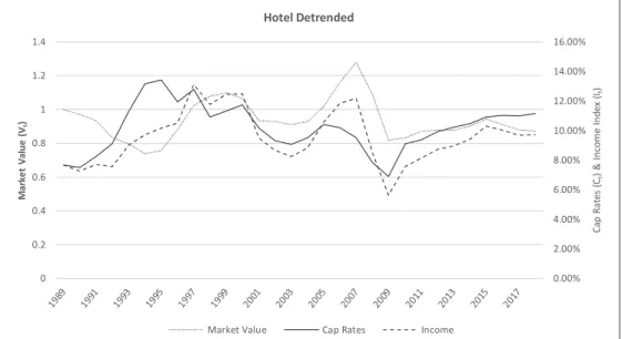
Hotel: Surprisingly, the hotel market values series had the lowest volatility of the five property types, somewhat contradicting the general thought that hotels are highly volatile properties. In our analysis, hotels exhibit just under half the total volatility (0.015) that the next most volatile

(20)

property-20 type, multifamily, does (0.027). Despite this, the individual contributions from income volatility (0.035) and cap rate volatility (0.027) are the highest across the analysis. So much in fact, that their individual shares are greater than 100% of the total volatility. This is made possible by the fact that there is a strong positive correlation (0.765) correlation between cap rates and income. A visual review of the hotel detrended NCREIF data shows (Figure V) income increasing through the 1990s then declining in the wake of the dot com bubble. Income then rises again during the economic expansion of the 2000s and sharply declines as a result of the great recession. Throughout all these variations, cap rates rise and fall absorbing nearly all the changes in income and keeping values within a relatively small band.

General Observations Across Property Types

To analyze differences across the five property types, we have grouped each series into one of three general categorizations. Those property types that exhibit a negative correlation between income (It) and cap rates (Ct), those that exhibit a positive correlation, and those that exhibit almost no

correlation.

The first group, which includes office, industrial, and retail, exhibits a negative correlation ranging from -0.158 to -0.644. Returning to our discussion about the interpretation of the model variables, we stated that a negative correlation between cap rates and income was an indication that investors tend to price a continuation of current space market trends into their valuations. Broadly, we believe that the fact that these three property types exhibit this behavior to be somewhat intuitive given their sensitivity to the broader economy. Demand for space in the office market is largely attributed to employment growth which is, like the broader economy, characterized by relatively long cycles. Reversals in office space demand tend to occur relatively infrequently making investors somewhat justified in their extrapolation of current trends. Similarly, industrial space, whether it is categorized as manufacturing or warehouse, is highly correlated with national economic production and also international trade. Finally, retail has obvious ties to the condition of the economy including consumption and consumer spending. We suspect that retail’s correlation between income and interest rates, which is the most negative of the five property types (-0.644), may be somewhat attributable to the prevalence of percentage lease structures. Percentage leases are effectively a revenue sharing contract between property owners and tenants. Whereas other property types may pay a fixed rent regardless of the condition of the underlying business or broader economy, retail property income should theoretically be more closely correlated with the tenant earnings. In that

(21)

21 sense, a strong correlation between income and cap rates is reasonable given the impact and relative speed at which broader economic trends could impact rent levels.

How well the negative correlation exhibited by these three property types can be explained by their respective space market fundamentals is an interesting topic, albeit one that is not germane to the focus of this paper, though it may be an area for additional study. Of more relevance to our topic is the fact that despite having the lowest income volatility of the five property types, office, industrial, and retail have the highest overall price volatility. Therefore, regardless of whether such behavior is justified, the tendency of investors to value these properties by extrapolating current space market trends exacerbates overall price volatility. In the context of our detrended NCREIF data, which has controlled the variance due to long-term secular trends, this is a powerful observation.

In contrast to office, industrial, and retail properties we found that multifamily exhibits the weakest correlation between cap rates and income on an absolute basis. Whereas a negative correlation in the first group seem to suggest extrapolation on the part of investors, this relatively weak relationship suggests a dislocation between the space and capital markets. As with the first group of properties, we find that this occurrence to be quite logical given investors’ perception of multifamily investment risk. As opposed to other property types that tend to fluctuate with the cyclical patterns of the wider economy, short-term leases and consistent (sometimes countercyclical) demand for housing are commonly thought to stabilize multifamily property income and values. While our data set may suggest that income volatility in multifamily is actually greater than other property types, if investors truly believe that multifamily income is stable in the long run, keeping cap rates relatively unchanged, even given income volatility, is a rational reflection of expected income normalization. This is

further supported by the fact that, although weakly correlated, multifamily cap rates and income covary positively, meaning investors tend to slightly temper the impact of income changes on valuations. As a result, multifamily investors’ expectation of mean reversion induces lower near-term volatility (valuation noise).

By contrast, hotel properties may represent an isolated case of this dynamic. Namely, that the short-term fluctuations that occur in income are, relative to other property types, so volatile that cap rates must effectively ‘float’ and covary to keep some stability in values. Put another way, it is investors’ expectation of future volatility in hotel income, rather than their expectation of mean reversion per se, that is reflected in correlations. In an appraisal-based index, this probably plays out more

(22)

22 seems to suggest the presence of a type of appraisal smoothing, in which the pronounced volatility of income requires a necessary adjustment on the part of appraisers to reflect the true long-term value of these properties.

Decomposing Volatility by Location (CBSA)

Results of the multifamily and office property variance decomposition by CBSA are shown in Table VI. We will not discuss the results of each CBSA decomposition individually but will describe some general observations.

Multifamily: In our analysis of multifamily price volatility by CBSA, we find that volatility is normally distributed around the mean (0.023), with Denver exhibiting the highest volatility (0.047) and Houston exhibiting the lowest volatility in market values (0.007). Income volatility is similarly distributed across CBSAs—Denver has the highest volatility of the group (0.056), while DC (0.010) shows the lowest volatility, though Houston closely follows (0.013). Average volatility directly attributed to variance in cap rates is roughly half that of income (0.011 vs. 0.024) but is further offset by the fact that across all of the CBSA’s included, income variance and cap rate variance are

positively correlated. As a result, income volatility constitutes the majority of overall volatility. In fact, in six of the ten CBSAs, income volatility is responsible for more than 100% of the overall volatility in market values.

Office: In reviewing the results of the office decomposition by geography, we find that price volatility (0.026) is slightly greater in magnitude than that of multifamily (0.023). The average across CBSAs is somewhat skewed by San Francisco (0.094), which has experienced very high volatility— almost ~3.0x the volatility of the next ranking New York (0.032). It should be noted, however, that San Francisco was disproportionately affected by the dot-com bubble, which began in Q4 2001, shortly after the start date of our analysis. Income as well as direct cap rate volatility follow a similar pattern, with most CBSAs falling below the average (0.019, 0.008) due to San Francisco’s outsized impact.

For a majority of the CBSAs included in the analysis, income contributes more than 50% of the price volatility. In Dallas and Chicago, income is responsible for more than 100% of price volatility. Overall, however, office tends to exhibit a more balanced split between income and cap rate

variance. The average correlation between income and cap rates across geographies is relatively weak (0.057), though this results from the fact that half of the CBSAs in our sample have a negative

(23)

23 correlation and half have a positive correlation. In reality, most CBSAs exhibit fairly significant positive or negative correlation, with the exception of San Francisco and to a lesser extent, Los Angeles.

General Observations Across Locations

Given the different time periods used between the property-type decomposition and the geographic decomposition, comparisons between the two analyses should be treated with caution. However, reviewing the results across the geographies in the context of this specific analysis, we observe a few trends. Generally, the more granular analysis of office and multifamily NCREIF series seem to support the findings in our property type decomposition. Investors in multifamily assets tend to price expected mean reversion into their valuations, as reflected in positive correlations across all CBSAs. There is some indication that lower barriers to supply growth may result in greater conservatism in valuations. Specifically, we find that plotting the correlation between income and cap rates (correlation[It, Ct)]) as a function of each CBSAs WLURI restrictive index, a measurement of the regulatory restrictiveness of residential development, shows a somewhat significant negative correlation. Lower index scores, representing less regulatory impeded areas, tend to be associated with higher mean reversion pricing (correlation[It, Ct]>0) (Figure VII).5 In this context, mean reversion pricing may reflect investors’ expectation that changes in income, at least positive changes in income, will more readily normalize in places where supply can be added to the market relatively easily.

Given that the office data exhibited both negative and positive correlations across CBSAs, a

simplified explanation of investor behavior is less easily derived and is most likely of lesser value. In fact, the dispersion of the CBSA data may suggest that our property level analysis of office is

somewhat muddled by opposing geographic trends embedded within the aggregate office data. With that being said, a cursory inspection of the office decomposition results suggests that locations with historically volatile employment growth such as Dallas, Houston and Chicago exhibit greater mean reversion pricing (Table VI).

As with the preceding analysis of price volatility by property type, by trying to explain the source of differences in valuation dynamics across locations, we risk clouding our holistic assessment of risk. Returning to the central premise of our paper, we note one final observation across both analyses.

5_{A simple linear regression of Corr(It,Ct) on the WLURI index yield suggests 25% of the variability in correlations can} be explained by the index score (R2_{= 0.25)}

(24)

24 Where investors value properties with an expectation of mean reverting income, as reflected in a positive correlation between income and cap rate variance, there is almost always lower price volatility. Alternatively, where investors incorporate a continuation of current income changes into valuations, as expressed through a negative correlation between income and cap rate variance, price volatility is almost always higher. To demonstrate the extent of this relationship, we have plotted the correlations of each data series (correlation[It, Ct)]) against the market value volatility (var[Vt]), for both the property type and CBSA analyses (Figure VIII). Regressing correlation on market value variance we find a negative relationship between the two variables (Table VII). If we consider the San Francisco office decomposition result to be an outlier and remove it from the regression analysis, the R2 _{increases from 0.11 to 0.25. If we further remove the Denver office decomposition} results, the R2 _{increases to 0.42. Though we must keep in mind that the two analyses were not} conducted over the same time period, we can see that this relationship generally holds across both our property type and location-based decompositions.

The significance of this observation is that at the aggregate level, investor expectations may play a greater role in pricing risk than actual realized changes in property fundamentals. We have shown that those classes of investment where fundamental income is expected to normalize experience less volatility over time, even if actual income variance relative to other property types or locations is relatively higher. The relationship is symmetrical, in that certain property types may experience higher price volatility despite having lower income volatility if investors in that asset class form valuations with an expectation that current changes in income will continue.

VI. Conclusion

Most research into the volatility of commercial real estate has focused on describing or quantifying how underlying changes in either the space market or asset market influence total return risk. Using a relatively simple stochastic framework, we have taken the analysis a step further to show

holistically how the relative contributions of each of those markets may explain higher or lower ex post market volatility. More importantly, however, we have shown how the expectations of investors who sit at the intersection of the space and asset markets, may play an overlooked role in

moderating or augmenting the relative risk associated with certain property types or locations. By specifically decomposing risk into its component variances as well as valuation driven covariances, we observed that is possible for investors’ perception of the underlying risk of an asset to dominate

(25)

25 realized risk in property fundamentals. While our results should certainly be considered in the

context of our data, which is largely comprised primarily appraised values, the widespread adoption of the NCRIEF NPI as a research and risk management tool means these observations should not be ignored.

(26)

26

VII. References

Campbell, John Y. “NBER Working Paper Series: A Variance Decomposition for Stock Returns.” Cambridge, MA: National Bureau of Economic Research, January 1990.

Campbell, Sean D., Morris A. Davis, Joshua Gallin, and Robert F. Martin. “What Moves Housing Markets: A Variance Decomposition of the Rent-Price Ratio.” Madison, WI: Wisconsin School of Business, June 2009.

Chan, K.C., Patric H. Hendershott, and Anthony B. Sanders. “Risk and Return on Real Estate: Evidence from Equity REITs.” NBER Working Paper Series. National Bureau of Economic Research, 1990.

Clayton, Jim, David C. Ling, and Andy Naranjo. “Commercial Real Estate Valuation: Fundamentals Versus Investor Sentiment.” Journal of Real Estate Finance & Economics 38, no. 1 (2009): 5–37. Conner, Phillip, and Youguo Liang. “The Complex Interaction Between Real Estate Cap Rates and

Interest Rates.” Briefings in Real Estate Finance 4, no. 3 (n.d.): 185–97.

Duca, John V., Patric H. Hendershott, and David C. Ling. “How Taxes and Required Returns Drove Commercial Real Estate Valuations Over the Past Four Decades.” National Tax Journal 70, no. 3 (September 2017): 549–83.

“Frequent Asked Questions About NCREIF and the NCREIF Property Index (NPI).” National Council of Real Estate Investment Fiduciaries, n.d.

Geltner, David. “Estimating Real Estate’s Systematic Risk from Aggregate Level Appraisal-Based.” Journal of the American Real Estate & Urban Economics Association 17, no. 4 (1989): 463–81.

———. “Smoothing in Appraisal-Based Returns.” Journal of Real Estate Finance & Economics 4, no. 3 (1991): 327–45.

Geltner, David, and Jiangpin Mei. “The Present Value Model with Time-Varying Discount Rates: Implications for Commercial Property Valuation and Investment Decisions.” Journal of Real Estate Finance & Economics 11, no. 2 (1995): 119–35.

Geltner, David, Norman Miller, Jim Clayton, and Eichholtz Piet. Commercial Real Estate Analysis and Investments. Third Edition. OH: OnCourse Learning, 2014.

Grenadier, Steven R. “The Persistence of Real Estate Cycles.” Journal of Real Estate Finance & Economics 10, no. 2 (1995): 95–119.

Gyourko, Joseph, Albert Saiz, and Anita A. Summers. “A New Measure of the Local Regulatory Environment for Housing Markets.” Urban Studies 45, no. 3 (2008): 693–729.

Kaliva, Kasimir, and Lasse Koskinen. “A Dynamic Model for Stock Market Risk Evaluation.” Finland Supervisory Authority, n.d.

(27)

27 Ling, David C., Andy Naranjo, and Scheick Benjamin. “Investor Sentiment, Limits to Arbitrage and

Private Market Returns.” Real Estate Economics 42, no. 3 (2014): 531–77.

Liu, Crocker H., and Jianping Mei. “An Analysis of Real-Estate Risk Using the Present Value Model.” Journal of Real Estate Finance & Economics 8, no. 1 (1994): 5–20.

Pagliari, Jr., Joseph L., Frederich Lieblich, Mark Schaner, and James R. Webb. “Twenty Years of the NCREIF Property Index.” Real Estate Economics 29, no. 1 (2001): 1–27.

“STAT 248: Removal of Trend & Seasonality Handout 4.” UC Berkeley, 2010.

https://www.stat.berkeley.edu/~gido/Removal%20of%20Trend%20and%20Seasonality.pdf. Wheaton, William. “The Volatility of Real Estate Markets: A Decomposition.” The Journal of Portfolio

(28)

28

VIII. Tables & Figures

Figure I

Market Value and Property Count for the NCREIF NPI 1978 – 2018

Figure II

NCREIF NPI Composition by Region 1978 – 2019

0 1,000 2,000 3,000 4,000 5,000 6,000 7,000 8,000 9,000 $0 $100 $200 $300 $400 $500 $600 $700 P ro pe rt y C ou nt M ar ke t V al ue ($ bn )

Market Value Prop Count

0% 10% 20% 30% 40% 50% 60% 70% 80% 90% 100% % o f N PI I nd ex b y P ro pe rt y C ou nt Multifamily

(29)

29 Figure II (Cont’d)

0% 10% 20% 30% 40% 50% 60% 70% 80% 90% 100% % o f N P I In de x by P ro pe rt y C ou nt Office

East Midwest South West

0% 10% 20% 30% 40% 50% 60% 70% 80% 90% 100% % o f N P I In de x by P ro pe rt y C ou nt Industrial

(30)

30 Figure II (Cont’d)

0% 10% 20% 30% 40% 50% 60% 70% 80% 90% 100% % o f N P I In de x by P ro pe rt y C ou nt Retail

East Midwest South West

0% 10% 20% 30% 40% 50% 60% 70% 80% 90% 100% % o f N P I In de x by P ro pe rt y C ou nt Hotel

(31)

31 Figure III

Aggregate (Trended) NCREIF NPI Data: 1989 – 2018

0.20 0.40 0.60 0.80 1.00 1.20 1.40 1.60 1.80 2.00

Market Value Index (vt)

Multifamily Office Industrial Retail Hotel

0.0% 2.0% 4.0% 6.0% 8.0% 10.0% 12.0% 14.0% Cap Rates (ct)

(32)

32 Figure III (Cont’d)

Aggregate (Trended) NCREIF NPI Data: 1989 – 2018

0.00 0.02 0.04 0.06 0.08 0.10 0.12 0.14 Income Index (it)

(33)

33 Figure IV

NCREIF NPI Market Values and Cap Rates: Original (Trended) vs. Detrended

0.20 0.40 0.60 0.80 1.00 1.20 1.40 1.60 1.80 2.00

Market Value: Multifamily

Trended (vt) Untrended (Vt) 0.20 0.40 0.60 0.80 1.00 1.20

Market Value: Office

Trended (vt) Untrended (Vt) 0.20 0.40 0.60 0.80 1.00 1.20 1.40 1.60

Market Value: Industrial

Trended (vt) Untrended (Vt) 0.00% 2.00% 4.00% 6.00% 8.00% 10.00% 12.00%

Cap Rates: Multifamily

Trended (ct) Untrended (Ct) 0.00% 2.00% 4.00% 6.00% 8.00% 10.00% 12.00%

Cap Rates: Office

Trended (ct) Untrended (Ct) 0.00% 2.00% 4.00% 6.00% 8.00% 10.00% 12.00%

Cap Rates: Industrial

(34)

34 Figure IV (Cont’d)

NCREIF NPI Market Values and Cap Rates: Original (Trended) vs. Detrended

0.20 0.40 0.60 0.80 1.00 1.20 1.40 1.60

Market Value: Retail

Trended (vt) Untrended (Vt) 0.20 0.40 0.60 0.80 1.00 1.20 1.40

Market Value: Hotel

Trended (vt) Untrended (Vt) 0.00% 2.00% 4.00% 6.00% 8.00% 10.00% 12.00%

Cap Rates: Retail

Trended (ct) Untrended (Ct) 0.00% 2.00% 4.00% 6.00% 8.00% 10.00% 12.00% 14.00% 16.00%

Cap Rates: Hotel

(35)

35 Figure V

Detrended Market Value Index (Vt), Income Index (It), and Cap Rates (Ct): 1989 – 2018

0.00% 2.00% 4.00% 6.00% 8.00% 10.00% 12.00% 0 0.2 0.4 0.6 0.8 1 1.2 Ca p Ra te s (Ct ) & In co m e In de x (It ) M ar ke t Va lu e (Vt ) Multifamily Detrended

Market Value Cap Rates Income

0.00% 2.00% 4.00% 6.00% 8.00% 10.00% 12.00% 0 0.2 0.4 0.6 0.8 1 1.2 Ca p Ra te s (Ct ) & In co m e In de x (It ) M ar ke t Va lu e (Vt ) Office Detrended

(36)

36 Figure V (Cont’d)

0.00% 2.00% 4.00% 6.00% 8.00% 10.00% 12.00% 0 0.2 0.4 0.6 0.8 1 1.2 Ca p Ra te s (Ct ) & In co m e In de x (It ) M ar ke t Va lu e (Vt ) Industrial Detrended

0.00% 2.00% 4.00% 6.00% 8.00% 10.00% 12.00% 0 0.2 0.4 0.6 0.8 1 1.2 Ca p Ra te s (Ct ) & In co m e In de x (It ) M ar ke t Va lu e (Vt ) Retail Detrended

(37)

37 Figure V (Cont’d)

Figure VI

10 Year US Treasury Yields: 1989 to 20186

6_{Source: US Department of the Treasury,} https://www.treasury.gov/resource-center/data-chart-center/interest-rates/Pages/default.aspx 0.00% 2.00% 4.00% 6.00% 8.00% 10.00% 12.00% 14.00% 16.00% 0 0.2 0.4 0.6 0.8 1 1.2 1.4 Ca p Ra te s (Ct ) & In co m e In de x (It ) M ar ke t Va lu e (Vt ) Hotel Detrended

0.0% 1.0% 2.0% 3.0% 4.0% 5.0% 6.0% 7.0% 8.0% 9.0% 10.0%

(38)

38 Figure VII

Multifamily Correlation (It,Ct) as a Function of WLURI Index Score by CBSA

Figure VIII

Correlation (It,Ct) vs. Variance (Vt) Regression7

7_{Includes results from part I and part II of analysis. Regression line plotted excludes the observations of San Francisco} (office) and Denver (multifamily)

0.10 0.20 0.30 0.40 0.50 0.60 0.70 0.80 -0.6 -0.4 -0.2 0 0.2 0.4 0.6 0.8 1 1.2 M ul tif am ily C or re la tio n( It ,C t)

WLURI Index Score Dallas Houston Atlanta Chicago DC Los Angeles Phoenix Denver Seattle New York 0 0.01 0.02 0.03 0.04 0.05 0.06 0.07 0.08 0.09 0.1 -1 -0.8 -0.6 -0.4 -0.2 0 0.2 0.4 0.6 0.8 1 1.2 Va ria nc e (V t) Correlation (It,Ct)

Property Type Office Multifamily Regression

San Francisco

(39)

39 Table I

NCREIF NPI Total Return Summary Statistics: 1989 – 2018

Table II

Cap Rate Comparison: CBRE H2 2018 Cap Rate Survey vs. 2018 NCREIF NPI Trailing Quarterly Cap Rate8

Property Type CBRE NCREIF Δ bps

Multifamily 5.4% 4.2% -124 Office 7.3% 4.3% -295 Industrial 6.3% 4.7% -161 Retail 6.9% 4.6% -235 Hotel 8.2% 7.5% -74 Mean 6.83% 5.06% -178

8_{Source: CBRE Cap Rate Survey - Second Half 2018, CBRE, Inc.}

% Share

Property Type Variance Std Deviation Income Valuation

Multifamily 0.00043 0.02083 3.7% 96.3%

Office 0.00072 0.02680 2.2% 97.8%

Industrial 0.00050 0.02241 2.7% 97.3%

Retail 0.00039 0.01967 2.5% 97.5%

(40)

40 Table III

Data Detrending OLS Regression Results

Intercept Slope (t)

Model Variable R2 _{Estimate Std Error T Value Estimate Std Error T Value} Multifamily Vt 0.836 -63.4100 5.4090 -11.720 0.0032 0.000 11.950 Office Vt 0.189 -12.7200 5.2760 -2.411 0.0007 0.000 2.554 Industrial Vt 0.457 -27.3400 5.8200 -4.697 0.0014 0.000 4.854 Retail Vt 0.649 -44.3600 6.3100 -7.030 0.0023 0.000 7.194 Hotel Vt 0.020 -2.9202 5.2041 -0.561 0.0002 0.000 0.747 Multifamily Ct 0.717 3.4030 0.3967 8.580 -0.0002 0.000 -8.416 Office Ct 0.520 2.6840 0.4754 5.646 -0.0001 0.000 -5.505 Industrial Ct 0.640 2.7840 0.3844 7.242 -0.0001 0.000 -7.054 Retail Ct 0.360 1.7490 0.4237 4.127 -0.0001 0.000 -3.970 Hotel Ct 0.317 2.6240 0.7045 3.725 -0.0001 0.000 -3.606 MF - DC Vt 0.148 -24.6100 15.0300 -1.637 0.0013 0.0007 1.718 MF - Los Angeles Vt 0.482 -46.9700 12.0900 -3.884 0.0024 0.0006 3.979 MF - Chicago Vt 0.803 -67.7000 8.2740 -8.182 0.0034 0.0004 8.326 MF - New York Vt 0.764 -53.1100 7.3230 -7.253 0.0027 0.0004 7.422 MF - Seattle Vt 0.756 -121.6000 16.9900 -7.160 0.0061 0.0008 7.262 MF - Dallas Vt 0.788 -128.1000 16.3800 -7.823 0.0065 0.0008 7.939 MF - San Francisco Vt 0.829 -75.4400 8.4430 -8.935 0.0038 0.0004 9.091 MF - Atlanta Vt 0.406 -57.5600 17.2700 -3.332 0.0029 0.0009 3.407 MF - Anaheim Vt 0.756 -107.4000 14.9800 -7.171 0.0054 0.0007 7.263 MF - Denver Vt 0.817 -107.5000 12.4900 -8.601 0.0054 0.0006 8.711 Office - DC Ct 0.618 4.1480 0.7820 5.305 -0.0002 0.0000 -5.245

Office - Los Angeles Ct 0.563 2.6630 0.5576 4.776 -0.0001 0.0000 -4.678

Office - Chicago Ct 0.672 2.9360 0.4879 6.017 -0.0001 0.0000 -5.902

Office - New York Ct 0.682 3.2950 0.5359 6.147 -0.0002 0.0000 -6.041

Office - Seattle Ct 0.624 3.1670 0.5873 5.392 -0.0002 0.0000 -5.310 Office - Dallas Ct 0.685 4.3160 0.7006 6.160 -0.0002 0.0000 -5.565 Office - SF Ct 0.680 2.6000 0.4245 6.124 -0.0001 0.0000 -6.004 Office - Atlanta Ct 0.451 2.4760 0.6489 3.815 -0.0001 0.0000 -3.733 Office - Anaheim Ct 0.398 2.5550 0.7457 3.426 -0.0001 0.0000 -3.351 Office - Denver Ct 0.649 2.7620 0.4835 5.713 -0.0001 0.0000 -5.609