HAL Id: hal-01354713
https://hal.archives-ouvertes.fr/hal-01354713
Submitted on 19 Aug 2016
HAL is a multi-disciplinary open access
archive for the deposit and dissemination of
sci-entific research documents, whether they are
pub-lished or not. The documents may come from
teaching and research institutions in France or
abroad, or from public or private research centers.
L’archive ouverte pluridisciplinaire HAL, est
destinée au dépôt et à la diffusion de documents
scientifiques de niveau recherche, publiés ou non,
émanant des établissements d’enseignement et de
recherche français ou étrangers, des laboratoires
publics ou privés.
TopPI: An Efficient Algorithm for Item-Centric Mining
Martin Kirchgessner, Vincent Leroy, Alexandre Termier, Sihem Amer-Yahia,
Marie-Christine Rousset
To cite this version:
Martin Kirchgessner, Vincent Leroy, Alexandre Termier, Sihem Amer-Yahia, Marie-Christine Rousset.
TopPI: An Efficient Algorithm for Item-Centric Mining. 18th International Conference on Big Data
Analytics and Knowledge Discovery, Sep 2016, Porto, Portugal. �10.1007/978-3-319-43946-4_2�.
�hal-01354713�
TopPI: An Efficient Algorithm for Item-Centric
Mining
Martin Kirchgessner1, Vincent Leroy1, Alexandre Termier2, Sihem
Amer-Yahia1, and Marie-Christine Rousset1
1
Université Grenoble Alpes, LIG, CNRS, Grenoble, France, [email protected],
2 Université Rennes 1, INRIA / IRISA, Rennes, France,
Abstract. We introduce TopPI, a new semantics and algorithm de-signed to mine long-tailed datasets. For each item, and regardless of its frequency, TopPI finds the k most frequent closed itemsets that item belongs to. For example, in our retail dataset, TopPI finds the itemset “nori seaweed, wasabi, sushi rice, soy sauce” that occurrs in only 133 store receipts out of 290 million. It also finds the itemset “milk, puff pastry”, that appears 152,991 times. Thanks to a dynamic threshold adjustment and an adequate pruning strategy, TopPI efficiently traverses the rele-vant parts of the search space and can be parallelized on multi-cores. Our experiments on datasets with different characteristics show the high per-formance of TopPI and its superiority when compared to state-of-the-art mining algorithms. We show experimentally on real datasets that TopPI allows the analyst to explore and discover valuable itemsets.
Keywords: Frequent itemset mining, Top-K, Parallel data mining
1
Introduction
Over the past twenty years, pattern mining algorithms have been applied suc-cessfully to various datasets to extract frequent itemsets and uncover hidden as-sociations [1,9]. As more data is made available, large-scale datasets have proven challenging for traditional itemset mining approaches. Indeed, the worst-case complexity of frequent itemset mining is exponential in the number of items in the dataset. To alleviate that, analysts use high threshold values and restrict the mining to the most frequent itemsets. But many large datasets exhibit a long tail distribution, characterized by the presence of a majority of infrequent items [5]. Mining at high thresholds eliminates low-frequency items, thus ignoring the ma-jority of them. In this paper we propose TopPI, a new semantics that is more appropriate to mining long-tailed datasets, and the corresponding algorithm.
A common request in the retail industry is finding a product’s associations with other products. This allows managers to obtain feedback on customer havior and to propose relevant promotions. Instead of mining associations be-tween popular products only, TopPI extracts itemsets for all items. By providing
the analyst with an overview of the dataset, it facilitates the exploration of the results.
We hence formalize the objective of TopPI as follows: extract, for each item, the k most frequent closed itemsets containing that item. This semantics raises a new challenge, namely finding a pruning strategy that guarantees correctness and completeness, while allowing an efficient parallelization, able to handle web-scale datasets in a reasonable amount of time. Our experiments show that TopPI can mine 290 million supermarket receipts on a single server. We design an algorithm that restricts the space of itemsets explored to keep the execution time within reasonable bounds. The parameter k controls the number of itemsets returned for each item, and may be tuned depending on the application. If the itemsets are directly presented to an analyst, k = 10 would be sufficient, while k = 500 may be used when those itemsets are post-processed.
The paper is organized as follows. Section 2 defines the new semantics and our problem statement. The TopPI algorithm is fully described in Section 3. In Section 4, we present experimental results and compare TopPI against a simpler solution based on TFP [6]. Related work is reviewed in Section 5, and we conclude in Section 6.
2
TopPI semantics
The data contains items drawn from a set I. Each item has an integer identifier, referred to as an index, which provides an order on I. A dataset D is a collection of transactions, denoted ht1, ..., tni, where tj ⊆ I. An itemset P is a subset of
I. A transaction tj is an occurrence of P if P ⊆ tj. Given a dataset D, the
projected dataset for an itemset P is the dataset D restricted to the occurrences of P : D[P ] = ht | t ∈ D ∧ P ⊆ ti. To further reduce its size, all items of P can be removed, giving the reduced dataset of P : DP = ht \ P | t ∈ D[P ]i.
The number of occurrences of an itemset in D is called its support, denoted supportD(P ). Note that supportD(P ) = supportD[P ](P ) = |DP|. An itemset P
is said to be closed if there exists no itemset P0 ⊃ P such that support (P ) = support (P0). The greatest itemset P0⊇ P having the same support as P is called the closure of P , further denoted as clo(P ). For example, in the dataset shown in Table 1a, the itemset {1, 2} has a support equal to 2 and clo({1, 2}) = {0, 1, 2}. Problem statement: Given a dataset D and an integer k, TopPI returns, for each item in D, the k most frequent closed itemsets (CIS) containing this item.
In this paper, we use TopPI to designate the new mining semantics, this prob-lem statement, and our algorithm. Table 1b shows the solution to this probprob-lem applied to the dataset in Table 1a, with k = 2. Note that we purposely ignore itemsets that occur only once, as they do not show a behavioral pattern.
As the number of CIS is exponential in the number of items, we cannot firstly mine all CIS and their support, then sort the top-k frequent ones for each item. The challenge is instead to traverse the small portions of the solutions space which contains our CIS of interest.
TID Transaction t0 {0, 1, 2} t1 {0, 1, 2} t2 {0, 1} t3 {2, 3} t4 {0, 3} (a) Input D
item top(i): P , support (P ) i 1st 2nd
0 {0}, 4 {0, 1}, 3 1 {0, 1}, 3 {0, 1, 2}, 2 2 {2}, 3 {0, 1, 2}, 2 3 {3}, 2
(b) TopPI results for k = 2
Table 1: Sample dataset
3
The TopPI algorithm
After an general overview in Section 3.1, this section details TopPI’s functions and their underlying principles. Section 3.2 shows how we shape the CIS (closed itemsets) space as a tree. Then Section 3.3 presents expand , TopPI’s tree traver-sal function. Section 3.4 shows an example travertraver-sal, to highlight the challenges of finding pruning opportunities specific to item-centric mining. The startBranch function, which implements the dynamic threshold adjustment, is detailed in Section 3.5. Section 3.6 presents the prune function and the prefix short-cutting technique, which allows TopPI to evaluate quickly and precisely which parts of the CIS tree can be pruned. We conclude in Section 3.7 by showing how TopPI can leverage multi-core systems.
3.1 Overview
TopPI adapts two principles from LCM [14] to shape the CIS space as a tree and enumerate CIS of high support first. Similarly to traditional top-k processing approaches [4], TopPI relies on heap structures to progressively collect its top-k results, and outputs them once the execution is complete. More precisely, TopPI stores traversed itemsets in a top-k collector which maintains, for each item i ∈ I, top(i ), a heap of size k containing the current version of the k most frequent CIS containing i. We mine all the k-lists simultaneously to maximize the amortization of each itemset’s computation. Indeed, an itemset is a candidate for insertion in the heap of all items it contains.
TopPI introduces an adequate pruning of the solutions space. For example, we should be able to prune an itemset {a, b, c} once we know it is not a top-k frequent for a, b nor c. However, as highlighted in the following example, we cannot prune {a, b, c} if it precedes interesting CIS in the enumeration. TopPI’s pruning function tightly cuts the CIS space, while ensuring results’ completeness. When pruning we can query the top-k-collector through min(top(i )), which is the kthsupport value in top(i ), or 2 if |top(i )| < k.
The main program, presented in Algorithm 1, initializes the collector in lines 2 and 3. Then it invokes, for each item i, startBranch(i , D, k ), which enumerates itemsets P such that max (P ) = i. In our examples, as in TopPI, items are
Algorithm 1: TopPI’s main function
Data: dataset D, integer k
Result: Output top-k CIS for all items of D
1 begin
2 foreach i ∈ I do // Collector instantiation
3 initialize top(i ), heap of max size k
4 foreach i ∈ I do // In increasing item order
5 startBranch(i, D, k)
represented by integers. While loading D, TopPI indexes items by decreasing frequency, hence 0 is the most frequent item. Items are enumerated in their natural order in line 4, thus items of greatest support are considered first.
TopPI does not require the user to define a minimum frequency, but we observe that the support range in each item’s top-k CIS varies by orders of magnitude from an item to another. Because filtering out less frequent items can speed up the CIS enumeration in some branches, startBranch implements a dynamic threshold adjustment. The internal frequency threshold, denoted ε, defaults to 2 because we are not interested in itemsets occurring once.
3.2 Principles of the closed itemsets enumeration
Several algorithms have been proposed to mine CIS in a dataset [6,12,13]. We borrow two principles from the LCM algorithm [14]: the closure extension, that generates new CIS from previously computed ones, and the first parent that avoids redundant computation.
Definition 1. An itemset Q ⊆ I is a closure extension of a closed itemset P ⊆ I if ∃e /∈ P , called an extension item, such that Q = clo(P ∪ {e}).
TopPI enumerates CIS by recursively performing closure extensions, starting from the empty set. In Table 1a, {0, 1, 2} is a closure extension of both {0, 1} and {2}. This example shows that an itemset can be generated by two different closure extensions. Uno et al. [14] introduced two principles which guarantee that each closed itemset is traversed only once in the exploration. We adapt their principles as follows. First, extensions are restricted to items smaller than the previous extension. Furthermore, we prune extensions that do not satisfy the first-parent criterion:
Definition 2. Given a closed itemset P and an item e /∈ P , hP, ei is the first parent of Q = clo(P ∪ {e}) only if max (Q \ P ) = e.
These principles shape the CIS space as a tree and lead to the following property: by extending P with e, TopPI can only recursively generate itemsets Q such that max (Q \ P ) = e. This property is extensively used in our algorithms, in order to predict which items can be impacted by recursions.
Both TopPI and LCM rely on the prefix extension and first parent test prin-ciples. However, in TopPI CIS are not outputted as they are traversed. They
are instead inserted in the top-k-collector. This allows TopPI to determine if deepening closure extensions may enhance results held in the top-k-collector, or if the corresponding sub-branch can be pruned. These two differences impact the execution of the CIS enumeration function.
3.3 CIS enumeration for item-centric mining
Algorithm 2: TopPI’s CIS exploration function 1 Function expand (P, e, DP, ε)
Data: CIS P , extension item e, reduced dataset DP, frequency threshold ε
Result: If he, P i is a relevant closure extension, collects CIS containing {e} ∪ P and items smaller than e
2 begin
3 Q ← closure({e} ∪ P ) // Closure extension
4 if max (Q \ P ) = e then // First-parent test
5 collect (Q, supportD(Q), true)
6 foreach i < e | support
DQ[i] ≥ ε do // In increasing item order 7 if ¬prune(Q, i, DQ, ε) then
8 expand (Q, i, DQ, ε)
TopPI traverses the CIS space with the expand function, detailed in Algo-rithm 2. expand performs a depth-first exploration of the CIS tree, and back-tracks when no frequent extensions remain in DJ (line 6). Additionally, in line 7
the prune function (presented in Section 3.6) determines if each recursive call may enhance results held in the top-k-collector, or if it can be avoided.
Upon validating the closure extension Q, TopPI updates top(i ), ∀ i ∈ Q, via the collect function (line 5). The support computation exploits the fact that supportD(Q) = supportDP(e), because Q = closure({e} ∪ P ). The last parameter of collect is set to true to point out that Q is a closed itemset (we show in Section 3.5 that it is not always the case).
When enumerating items in line 6, TopPI relies on the items’ indexing by decreasing frequency. As extensions are only done with smaller items this ensures that, for any item i ∈ I, the first CIS containing i enumerated by TopPI combine i with some of the most frequent items. This heuristic increases their probability of having a high support, and overall raises the support of itemsets in the top-k-collector.
In expand , as in all functions detailed in this paper, operations like computing clo(P ) or DP rely on an item counting over the projected dataset D[P ]. Because
it is resource-consuming, in our implementation item counting is done only once over each D[P ], and kept in memory while relevant. The resulting structure and accesses to it are not explicited for clarity.
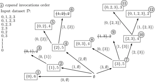
3.4 Finding pruning opportunities in an example enumeration We now discuss how we can optimize item-centric mining in the example CIS enumeration of Figure 1, when k = 2. Items are already indexed by decreasing
frequency. Candidate extensions of steps 3 and 9 are not collected as they fail the first-parent test (their closure is {0, 1, 2, 3}).
Input dataset D: 0, 1, 2, 3 0, 1, 2, 3 0, 2, 3 2, 3 0, 2 0, 3 1 1 1 0
i expand invocations order
∅ {0}, 6 1 h0, ∅i {1}, 5 2 h1, ∅i {0, 1}, 23 h0, {1}i {2}, 5 4 h2, ∅i {0, 2}, 4 5 h0, {2}i {1, 2}, 26 h1, {2}i {3}, 5 h3, ∅i {0, 3}, 48 h0, {3}i {1, 3}, 2 9 h1, {3}i {2, 3}, 410 h2, {3}i 7 {0, 2, 3}, 3 11 h0, {2, 3}i {0, 1, 2, 3}, 212 h1, {2, 3}i
Fig. 1: An example dataset and its corresponding CIS enumeration tree with our expand function. Each node is an itemset and its support. hi, P i denotes the closure extension operation. Striked out itemsets are candidates failing the first-parent test (Algorithm 2, line 4).
In frequent CIS mining algorithms, the frequency threshold allows the pro-gram to lighten the intermediate datasets (DQ) involved in the enumeration. In
TopPI our goal is to increase ε above 2, in some branches. In our example, before step 4 we can compute items’ supports in D[2] — these supports are re-used in
expand (∅, 2, D, ε) — and observe that the two most frequent items in D[2] are 2 and 0, with respective supports of 5 and 4. These will yield two CIS of supports 5 and 4 in top(2). The intuition of dynamic threshold adjustment is that 4 might therefore be used as a frequency threshold in this branch. It is not possible in this case because a future extension, 1, does not have its k itemsets at step 4.
This is also the case at step 7. The dynamic threshold adjustment done by the
startBranch function takes this into account.
After step 8, top(0), top(2) and top(3) already contain two CIS, as required,
all having a support of 4 or more. Hence it is tempting to prune the extension h{3}, 2i (step 10), as it cannot enhance top(2) nor top(3). However, at this step, top(1) only contains a single CIS and 1 is a future extension. Hence 10 cannot be pruned: although it yields an useless CIS, one of its extensions leads to a useful one (step 12). In this tree we can only prune the recursion towards step 11.
This example’s distribution is unbalanced in order to show TopPI’s corner cases with only 4 items; but in real datasets, with hundreds of thousands of items,
such cases regularly occur. This shows that an item-centric mining algorithm requires rigorous strategies for both pruning the search space and filtering the datasets.
3.5 Dynamic threshold adjustment
If we initiate each CIS exploration branch by invoking expand (∅, i , D, 2 ), ∀i ∈ I, then prune would be inefficient during the k first recursions — that is, until top(i) contains k CIS. For frequent items, which yield the biggest projected datasets, letting the exploration deepen with a negligible frequency threshold is particularly expensive. Thus it is crucial to diminish the size of the dataset as often as possible, by filtering out less frequent items that do not contribute to our results. Hence we present the startBranch function, in Algorithm 3, which performs the dynamic threshold adjustment and avoids the cold start situation.
Algorithm 3: TopPI’s CIS enumeration branch preparation 1 Function startBranch(i , D, k )
Data: root item i, dataset D, integer k
Result: Enumerates CIS P such that max (P ) = i
2 begin
3 foreach j ∈ topDistinctSupports(D[i], k) do // Pre-filling with partial itemsets
4 collect ({i, j}, supportD[i](j), false)
5 εi← minj≤i(min(top(j ))) // Dynamic threshold adjustment 6 expand (∅, i, D, εi)
Given a CIS {i} and an extension item e < i, computing Q = clo({e} ∪ {i}) is a costly operation that requires counting items in D{i}[e]. However we observe
that support (Q) = supportD({e} ∪ {i}) = supportD[i](e), and the latter value is computed by the items counting, prior to the instantiation of D{i}. Therefore,
when starting the branch of the enumeration tree rooted at i, we can already know the supports of some of the upcoming extensions.
The function topDistinctSupports counts items’ frequencies in D[i] — result-ing counts are re-used in expand for the instantiation of D{i}. Then, in lines 3–4, TopPI considers items j whose support in D[i] is one of the k greatest, and stores the partial itemset {i, j} in the top-k collector (this usually includes {i} alone). We call these itemsets partial because their closure has not been evaluated yet, so the top-k collector marks them with a dedicated flag: the third argument of collect is false (line 4). Later in the exploration, these partial itemsets are ei-ther ejected from top(i ) by more frequent CIS, or replaced by their closure upon its computation (Algorithm 2, line 5).
Thus top(i ) already contains k itemsets at the end of the loop of lines 3– 4. The CIS recursively generated by the expand invocation (line 6) may only contain items lower than i. Therefore the lowest min(top(j )), ∀j ≤ i, can be used as a frequency threshold in this branch. TopPI computes this value, εi, on
Algorithm 4: TopPI’s pruning function
1 Function prune(P , e, DP, ε)
Data: itemset P , extension item e, reduced dataset DP, minimum support
threshold ε
Result: true if expand (P , e, DP, ε) will not provide new results to the
top-k-collector, false otherwise
2 begin
3 if supportDP({e})) ≥ min(top(e)) then
4 return false
5 foreach i ∈ P do
6 if supportDP({e})) ≥ min(top(i )) then
7 return false
8 foreach i < e | supportDP(i) ≥ ε do
9 bound ← min(supportDP({i }), supportDP({e}))
10 if bound ≥ min(top(i )) then
11 return false
12 return true
because min(top(i )) is relatively high for more frequent items. Thus TopPI can filter the biggest projected datasets as a frequent CIS miner would.
Note that two partial itemsets {i, j} and {i, l} of equal support may in fact have the same closure {i, j, l}. Inserting both into top(i ) could lead to an overes-timation of the frequency threshold and trigger the pruning of legitimate top-k CIS of i. This is why TopPI only selects partial itemsets with distinct supports.
3.6 Pruning function
As shown in the example of Section 3.4, TopPI cannot prune a sub-tree rooted at P by observing P alone. We also have to consider itemsets that could be enumerated from P through first-parent closure extensions. This is done by the prune function presented in Algorithm 4. It queries the collector to determine whether expand (P, e, DP, ε) and its recursions may impact the top-k results of
an item. If it is not the case then prune returns true, thus pruning the sub-tree rooted at clo({e} ∪ P ).
The anti-monotony property [1] ensures that the support of all CIS enu-merated from he, P i is smaller than supportDP({e}). It also follows from the definition of expand that the only items potentially impacted by the closure ex-tension he, P i are in {e} ∪ P , or are inferior to e. Hence we check supportDP({e}) against top(i ) for all concerned items i.
The first case, considered in lines 3 and 5, checks top(e) and top(i ), ∀i ∈ P . Smaller items, which may be included in future extensions of {e} ∪ P , are considered in lines 8–11. It is not possible to know the exact support of these CIS, as they are not yet explored. However we can compute, as in line 9, an upper bound such that bound ≥ support (clo({i, e} ∪ P )). If this bound is smaller than min(top(i)), then extending {e} ∪ P with i cannot provide a new CIS to
top(i). Otherwise, as tested in line 10, we should let the exploration deepen by returning false. If this test fails for all items i, then it is safe to prune because all top(i) already contain k itemsets of greater support.
The inequalities of lines 3, 6 and 10 are not strict to ensure that no partial itemset (inserted by the startbranch function) remains at the end of the explo-ration. We can also note that the loop of lines 8–11 may iterate on up to |I| items, and thus may take a significant amount of time to complete. Hence our implementation of the prune function includes an important optimization.
Avoiding loops with prefix short-cutting: we can leverage the fact that TopPI enumerates extensions by increasing item order. Let e and f be two items suc-cessively enumerated as extensions of a CIS P (Algorithm 2 line 6). As e < f , in the execution of prune(P, f, DP, ε) the loop of lines 8–11 can be divided into
iterations on items i < e ∧ i 6∈ P , and the last iteration where i = e. We observe that the first iterations were also performed by prune(P, e, DP, ε), which can
therefore be considered as a prefix of the execution of prune(P, f, DP, ε).
To take full advantage of this property, TopPI stores the smallest bound com-puted line 9 such that prune(P, ∗, DP, ε) returned true, denoted boundmin(P ).
This represents the lowest known bound on the support required to enter top(i), for items i ∈ DP ever enumerated by line 8. When evaluating a new extension f
by invoking prune(P, f, DP, ε), if supportDP(f ) ≤ boundmin(P ) then f cannot satisfy tests of lines 6 and 10. In this case it is safe to skip the loop of lines 5–7, and more importantly the prefix of the loop of lines 8–11, therefore reducing this latter loop to a single iteration. As items are sorted by decreasing frequency, this simplification happens very frequently.
Thanks to prefix short-cutting, most evaluations of the pruning function are reduced to a few invocations of min(top(i )). This allows TopPI to guide the itemsets exploration with a negligible overhead.
3.7 Parallelization
As shown by Négrevergne et al. [11], the CIS enumeration can be adapted to shared-memory parallel systems by dispatching startBranch invocations (Algo-rithm1, line 5) to different threads. When multi-threaded, TopPI ensures that the dynamic threshold computation (Algorithm 3, line 5) can only be executed for an item i once all items lower than i are done with the top-k collector pre-filling (Algorithm 3, line 3).
Sharing the collector between threads does not cause any congestion because most accesses are read operations from the prune function. Preliminary experi-ments, not included in this paper for brevity, show that TopPI shows an excellent speedup when allocated more CPU cores. Thanks to an efficient evaluation of prune, the CIS enumeration is the major time consuming operation in TopPI.
4
Experiments
We now evaluate TopPI’s performance and the relevance of its results, with three real-life datasets on a multi-core machine. We start by comparing its performance to a simpler solution using a global top-k algorithm, in Section 4.1. Then we observe the impact of our optimizations on TopPI’s run-time, in Section 4.2. Finally Section 4.3 provides a few itemsets examples, confirming that TopPI highlights patterns of interest about long tailed items. We use 3 real datasets:
– Tickets is a 24GB retail basket dataset collected from 1884 supermarkets over a year. There are 290,734,163 transactions and 222,228 items.
– Clients is Tickets grouped by client, therefore transactions are two to ten times longer. It contains 9,267,961 transactions in 13.3GB, each representing the set of products bought by a single customer over a year.
– LastFM is a music recommendation website, on which we crawled 1.2 million public profile pages. This results in a 277MB file where each transaction contains the 50 favorite artists of a user, among 1.2 million different artists. All measurements presented here are averages of 3 consecutive runs, on a single machine containing 128GB of RAM and 2 Intel Xeon E5-2650 8-cores CPUs with Hyper Threading. We implemented TopPI in Java and will release its source upon the publication of this paper.
4.1 Baseline comparison
We start by comparing TopPI to its baseline, which is the most straightfor-ward solution to item-centric mining: it applies a global top-k CIS miner on the projected dataset D[i], for each item i in D occurring at least twice.
We implemented TFP[6], in Java, to serve as the top-k miner. It has an additional parameter lmin, which is the minimal itemset size. In our case lmin
is always equal to 1 but this is not the normal use case of TFP. For a fair comparison, we added a major pre-filtering: for each item i,we only keep items having one of the k highest supports in D[i]. In other words, the baseline also benefits from a dynamic threshold computation. This is essential to its ability to mine a dataset like Tickets. The baseline also benefits from the occurrence delivery provided by our input dataset implementation (ie. instant access to D[i]). Its parallelization is obvious, hence both solutions use all physical cores available on our machine.
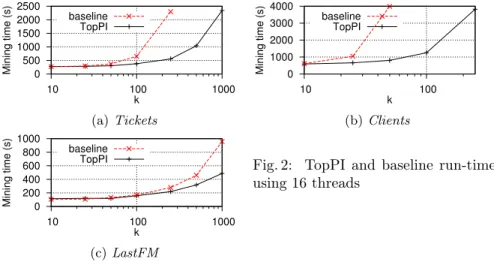
Figure 2 shows the run-times on our datasets when varying k. Both solutions are equally fast for k = 10, but as k increases TopPI shows better performance. The baseline even fails to terminate in some cases, either taking over 8 hours to complete or running out of memory. Instead TopPI can extract even 500 CIS per item out of the 290 million receipts of Tickets in less than 20 minutes, or 500 CIS per item out of Clients in 3 hours.
For k ≥ 200, as the number of items having less than k CIS increases, more and more CIS branches have to be traversed completely. This explains the expo-nential increase of run-time. However we usually need 10 to 50 CIS per item, in
0 500 1000 1500 2000 2500 10 100 1000 Mining time (s) k TopPI baseline (a) Tickets 0 1000 2000 3000 4000 10 100 Mining time (s) k TopPI baseline (b) Clients 0 200 400 600 800 1000 10 100 1000 Mining time (s) k TopPI baseline (c) LastFM
Fig. 2: TopPI and baseline run-times using 16 threads
which case such complete traversals only happens in extremely small branches. During this experiment, TopPI’s memory usage remains reasonable: below 50GB for Tickets, 30GB for Clients and 10GB for LastFM.
We also observe that the baseline enumerates many more intermediate solu-tions. Ideally, an algorithm would only enumerate outputted solusolu-tions. But, as shown in Section 3.4, item-centric mining requires the enumeration of a few ad-ditional itemsets to reach some solutions. On LastFM, when k = 100, the output contains approximately 12.8 million distinct itemsets. The baseline enumerated 50.6 million itemsets and TopPI only 17.4 millions. As each D[i] is mined in-dependently for all items i, the baseline cannot amortize results from a branch to another, so this result would likely be also observed with another top-k CIS mining algorithm. This highlights the need for a specific item-centric CIS mining algorithm. Thanks to the use of appropriate heuristics to guide the exploration, TopPI only enumerates a small fraction of discarded itemsets.
These results show that TopPI is fast and scalable. Even on common hard-ware: TopPI is able to mine LastFM with k = 50 and ε = 2 on a laptop with 4 threads (Intel Core i7-3687U) and 6 GB of RAM in 16 minutes.
4.2 Contributions impact
We now validate the individual impact of our contributions: the dynamic thresh-old adjustment in startBranch, described in Section 3.5, and the prefix short-cutting in prune, presented at the end of Section 3.6. To do so, we make these features optional in TopPI’s implementation and evaluate their impact on the execution time. Finally we disable both features, to observe how TopPI would perform as a simple pruning by top-k-collector polling in LCM.
Table 2 compares the run-time measured for these variants against the fully optimized version of TopPI’s, on all our datasets when using the full capacity of our server. We use k = 50, which is sufficient to provide interesting results.
Dataset Complete TopPI Without dynamic Without prefix Without both threshold adjustment short-cutting
Tickets 222 1136 (×5) 230 (+4%) 13863 (3.8 hours, ×62)
Clients 661 Out of memory 4177 (×6) Out of memory
LastFM 116 177 (+53%) 150 (+29%) 243 (×2)
Table 2: TopPI run-times (in seconds) on our datasets, using 32 threads and k = 50, when we disable the operations proposed in Section 3.
Disabling dynamic threshold adjustment implies that all projected datasets created during the CIS exploration carry more items. Hence intermediate datasets are bigger. This slows down the exploration but also increase the memory con-sumption. Therefore, without dynamic threshold adjustment, the TFP-based baseline presented in the previous experiment cannot run (on our 3 datasets) and TopPI also runs out of memory on Clients.
When we disable prefix short-cutting in the prune function, it has to evaluate more extensions in Algorithm 4, lines 8–11. Hence we observe greater slowdowns on datasets having longer transactions: on average, transactions contain 12 items in Tickets, 50 items in LastFM , and 213 in Clients.
The prune function is even more expensive if we disable both optimizations, as potential extensions are not only all evaluated but also more numerous. This experiment shows that it’s the combined usage of dynamic threshold adjustment and prefix short-cutting that allows TopPI to mine large datasets efficiently.
4.3 Example itemsets
From Tickets: Itemsets with high support can be found for very common prod-ucts, such as milk: “milk, puff pastry” (152,991 occurrences), “milk, eggs” (122,181) and “milk, chocolate spread” (98,982). Although this particular milk product was bought 5,402,063 times (i.e. in 1.85% of the transactions), some of its top-50 as-sociated patterns would already be out of reach of traditional CIS algorithms: “milk, chocolate spread” appears in 0.034% transactions.
Interesting itemsets can also be found for less frequent (tail) products. For example, “frangipane, puff pastry, sugar” (522), shows the basic ingredients for french king cake. We also found evidence of some sushi parties, with itemsets such as “nori seaweed, wasabi, sushi rice, soy sauce” (133). We observe similar patterns in Clients.
From LastFM: TopPI finds itemsets grouping artists of the same music genre. For example, the itemset “Tryo, La Rue Ketanou, Louise Attaque” (789 occurrences), represents 3 french alternative bands. Among the top-10 CIS that contain “Var-doger” (a black-metal band from Norway which only occurs 10 times), we get the itemset “Vardoger, Antestor, Slechtvalk, Pantokrator, Crimson Moonlight” (6 occurrences). TopPI often finds such itemsets, which, in the case of unknown artists, are particularly interesting to discover similar bands.
5
Related Work
The first algorithms in the field were frequent itemsets mining algorithms, whose parameter is a minimum support threshold. By definition, items that belong to the long tail are excluded from their results. Generate-and-test approaches like Apriori [1], if we want to keep a majority of items in the results, cannot be used on our datasets because the candidate generation would exhaust our machines’ capacity. Pasquier et al. identified closed itemsets [12], which are less numerous while conveying the same information. CLOSET [13] is a CIS mining algorithm which uses prefix trees to store the initial and projected datasets. However prefix trees’ instantiation is not amortized on our datasets, where between 90% (Tick-ets) and 99% (Clients, LastFM) of transactions are unique. Hence TopPI inherits its CIS enumeration from LCM [14], whose structures (transactions concatenated in an array) are straightforward and CPU cache-friendly.
Given a new dataset, it can be difficult to select an appropriate minimum frequency threshold. Therefore Han et al. therefore proposed TFP [6], an algo-rithm that returns the k most frequent closed itemsets in D containing at least lmin items. We show in Section 4.1 how it can be adapted to emulate TopPI,
but is not as robust. In particular, this method runs out of memory if we do not let it benefit from our dynamic threshold adjustment.
TopPI relies on frequency to rank each k itemsets associated with an item. Another possibility could be to rank them by statistical correlation with the item, for example by p-value. But it implies the search of an adequate (usually low) frequency threshold, as in LAMP [10], which is not affordable at our scale. Le Bras et al. show how 13 other quality measures can be integrated in a generate-and-test mining algorithm [8]. But, as with Apriori, the candidate generation step is unfeasible at our scale. As TopPI is able to analyze a year of activity of 1884 supermarkets in minutes on a single server, ranking by p-value (or another quality measure) can instead be implemented as a post-processing of TopPI’s results. We discuss in [7] which quality measures are adapted to retail data.
To the best of our knowledge, PFP [9] is the only other centric item-set mining algorithm: it returns a maximum of k itemitem-sets per item. However PFP does not ensure that these itemsets are the most frequent, nor that they are closed, and is developed for the MapReduce platform [3]. Preliminary ex-periments, not shown here due to space restrictions, show that a single server running TopPI can outperform a 50 machines cluster running PFP.
6
Conclusion
To the best of our knowledge, TopPI is the first algorithm to formalize and solve at scale the problem of mining item-centric top-k closed itemsets, a semantic more appropriate to mining long-tailed datasets. TopPI is able to operate effi-ciently on long tail content, which is out of reach of standard mining and global top-k algorithms. Instead of generating millions of itemsets only containing the very few frequent items, TopPI spreads its exploration evenly to mine a fixed
number of k itemsets for each item in the dataset, including rare ones. This is particularly important in the context of Web datasets, in which the long tail contains most of the information [5], and in the retail industry, where it can account for a large fraction of the revenue [2].
Acknowledgments: This work was partially funded by the Datalyse PIA project.
References
1. Agrawal, R., Srikant, R.: Fast algorithms for mining association rules in large databases. In: Proceedings of the 20th International Conference on Very Large Data Bases (VLDB). pp. 487–499 (1994)
2. Anderson, C.: The Long Tail: Why the Future of Business Is Selling Less of More. Hyperion (2006)
3. Dean, J., Ghemawat, S.: Mapreduce: simplified data processing on large clusters. In: Proceedings of the 6th Symposium on Operating System Design and Imple-mentation (OSDI) (2004)
4. Fagin, R., Lotem, A., Naor, M.: Optimal aggregation algorithms for middleware. In: Proc. of the Symp. on Principles of Database Systems (PODS) (2001) 5. Goel, S., Broder, A., Gabrilovich, E., Pang, B.: Anatomy of the long tail:
ordi-nary people with extraordiordi-nary tastes. In: Proceedings of the Third International Conference on Web Search and Data Mining (WSDM). pp. 201–210 (2010) 6. Han, J., Wang, J., Lu, Y., Tzvetkov, P.: Mining top-k frequent closed patterns
without minimum support. In: Proceedings of the International Conference on Data Mining (ICDM). pp. 211–218. IEEE (2002)
7. Kirchgessner, M., Mishra, S., Leroy, V., Amer-Yahia, S.: Testing interestingness measures in practice: A large-scale analysis of buying patterns. http://arxiv. org/abs/1603.04792 (2016)
8. Le Bras, Y., Lenca, P., Lallich, S.: Mining interesting rules without support re-quirement: a general universal existential upward closure property, Annals of in-formation systems, vol. 8, chap. Data Mining, pp. 75–98. Springer (2010)
9. Li, H., Wang, Y., Zhang, D., Zhang, M., Chang, E.Y.: Pfp: parallel fp-growth for query recommendation. In: Proceedings of the second conference on Recommender systems (RecSys). pp. 107–114 (2008)
10. Minato, S.I., Uno, T., Tsuda, K., Terada, A., Sese, J.: A fast method of statistical assessment for combinatorial hypotheses based on frequent itemset enumeration. In: Machine Learning and Knowledge Discovery in Databases, vol. 8725, pp. 422– 436. Springer (2014)
11. Négrevergne, B., Termier, A., Méhaut, J.F., Uno, T.: Discovering closed frequent itemsets on multicore: Parallelizing computations and optimizing memory accesses. In: Proceedings of the International Conference on High Performance Computing and Simulation (HPCS). pp. 521–528 (2010)
12. Pasquier, N., Bastide, Y., Taouil, R., Lakhal, L.: Discovering frequent closed item-sets for association rules. In: Proceedings of the 7th International Conference on Database Theory (ICDT). pp. 398–416 (1999)
13. Pei, J., Han, J., Mao, R.: Closet: An efficient algorithm for mining frequent closed itemsets. In: ACM SIGMOD workshop on research issues in data mining and knowl-edge discovery. vol. 4, pp. 21–30 (2000)
14. Uno, T., Asai, T., Uchida, Y., Arimura, H.: An efficient algorithm for enumerating closed patterns in transaction databases. In: Discovery Science. pp. 16–31 (2004)