HAL Id: hal-01385572
https://hal.archives-ouvertes.fr/hal-01385572
Submitted on 21 Oct 2016
HAL is a multi-disciplinary open access
archive for the deposit and dissemination of
sci-entific research documents, whether they are
pub-lished or not. The documents may come from
teaching and research institutions in France or
abroad, or from public or private research centers.
L’archive ouverte pluridisciplinaire HAL, est
destinée au dépôt et à la diffusion de documents
scientifiques de niveau recherche, publiés ou non,
émanant des établissements d’enseignement et de
recherche français ou étrangers, des laboratoires
publics ou privés.
A comparative study of low sampling non intrusive load
dis-aggregation
Kaustav Basu, Ahmad Hably, Vincent Debusschere, Seddik Bacha, Geert Jan
Dirven, Andres Ovalle
To cite this version:
Kaustav Basu, Ahmad Hably, Vincent Debusschere, Seddik Bacha, Geert Jan Dirven, et al.. A
comparative study of low sampling non intrusive load dis-aggregation. IECON 2016 - 42nd Annual
Conference of the IEEE Industrial Electronics Society, Oct 2016, Florence, Italy. �hal-01385572�
1
A comparative study of low sampling non intrusive
load dis-aggregation
Kaustav Basu, Ahmad Hably, Vincent Debusschere, Seddik Bacha, Geert Jan Dirven, Andres Ovalle
Abstract—Non-intrusive load monitoring (NILM) deals with the identification and subsequent energy estimation of the indi-vidual appliances from the smart meter data. The state of the art applications typically runs once per day and reports the detected appliances. In this work, data driven models are implemented for two different sampling rates (10 seconds and 15 minutes). The models are trained for 20 houses in the Netherlands and tested for a period of 4-weeks. The results indicate that the disaggregation methods is applicable for both sampling cases but with different use-case.
Index Terms—Non-intrusive load monitoring, load disaggre-gation, Signal Processing, Smart Meters, Energy Management, Smart Grids.
I. INTRODUCTION
Smart meters are getting deployed worldwide on a large scale. This large scale generation of digital energy data mandates a deeper look inside the consumption patterns of different appliances present inside the house. The insight into the residential load consumption has advantages for both the energy utility provider as well as for the consumer. In the context of smart grids, insights on the energy consumption patterns through appliance usage helps to manage the energy distribution [1], [2], especially for the integration of more fluctuating energy sources (i.e. renewable). The strategies commonly employed are demand response to reduce peak demand by eliminating electricity use, or by shifting it to non-peak times [3], [4]. The time of use pricing has also been successfully employed to this end. From the point of view of energy providers, load identification can also play an important part in future prediction of usages of particular appliances where the process of historical data collection is made as less intrusive as possible [5], [6]. The current smart meters are capable to report the total electrical load, to further develop energy management strategies, appliance usage insight needs to be provided. The appliances in the residence could be directly monitored but the associated cost and inconvenience to be used are the primary reasons that smart meters are unable to succeed in the market. Non-intrusive methods propose an attractive alternative with reduced cost and manual overheads. To achieve this goal new data analysis mechanisms have to be proposed to inhabitants for their satisfaction and energy costs reduction. Just a transfer from an analogue to a digital system is not good enough for the customers. A comprehensive and qualitative data analysis mechanism has to be proposed
K. Basu, A. Hably, V. Debusschere, S. Bacha and Andres Ovalle are with the Grenoble Alpes University - G2ELab, France. e-mail: ahmad.hably @gipsa-lab.grenoble-inp.fr
GJ. Dirven is the CEO of Greeniant B.V
coupled with the subsequent load management strategies. The residential building’s sector is mainly considered in this work but the tools and methodology are fully applicable to any other kind of buildings. Next to the efforts necessary on the data-acquisition side, it is equally important to develop necessary insights in consumer needs. The NILM technologies heavily rely on the granularity of data. This work primarily digs deep into the two commonly found sampling rates and highlights the use cases that can be generated from it. The methodology used is data driven and focuses on the fundamental signal parameters that differentiates between appliances.
II. PASTWORK
The NILM can broadly segmented into six data flow phases [7], namely, data acquisition followed by data processing, event detection, feature extraction, event classification and finally energy computation.
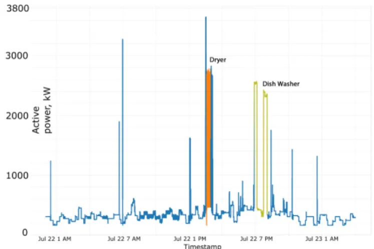
In the early 90’s one of the pioneering work in load dis-aggregation was published [8]. It proposed to identify ap-pliances by their respective ON/OFF transitions. It tried to consider power consumption changes (i.e. events) both in the active and reactive power of the signal. The current output of a NILM algorthm, indentfying the various high consuming appliances in the residence is shown in Fig. 1. Methods were
Fig. 1: Non-Intrusive Load Monitoring (blue: no appliances detected).
then proposed to identify individual appliances from their On/Off transitions. From that time, most of the approaches were event-based and at a high sampling rate, typically less than one second. Even though is considered one field, there are two fundamentally different directions. The main difference
is in the granularity of the energy data that is considered, which drives the use of tools and analysis techniques. The two granularities are approximately:
• High sampling rate ≥50 Hz (≤ 0.02 s) (up to several kHz).
• Low sampling rate ≤1 Hz (≥ 1 s).
Signals are primarily analysed using event and non-event based techniques. All high sampling rate data are generally analysed using event based techniques but in the low sampling case it is analysed by both event based and non-event based techniques. These techniques are discussed in details in the following sections.
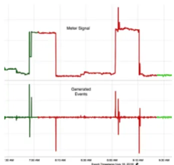
1) High sampling rate NILM (event based): High-frequency measurements allow the analysis of not just the energy used, but also the analysis of the structure of the current-voltage waveform itself [9]. Running different appli-ances introduce different signatures of disturbappli-ances of the pure sine waveform, which can be used to disaggregate them. Getting this high-frequency data requires specializing measuring equipment such as current clamp. In [10], a method has been proposed to generate signatures based on the active power range, reactive power range, harmonic content range, with or without spike, single phase or double-phase and searching time. Approaches typically consist of identifying the steady state or in some cases transient state features [11], [12]. Subsequently, these signatures are matched with earlier learned models using a pattern recognition algorithm [13], [14]. The drawbacks of these approaches are mainly hardware requirement due to high sampling rates and the impracticality of the process being totally non-intrusive [15], [16]. These methods do not fit well into the smart meter sampling rate, so separate device has to be installed for training, visualisation and communication to the grid. This is a major drawback for these methods, commercially and practically speaking. The load separation at a high sampling rate of all the appliances also raise privacy concerns as user activity can be easily detected, interpreted and monitored [7]. The techniques rely on first identifying the power level transition of different appliances which in the NILM literature is called events. In Fig. 2 the event based technique is shown. Fig. 2a shows the generic appliance On/Off locations which are identified and subsequently matched to detect the appliance.
2) Low sampling rate NILM (event and non-event based): Low-frequency measurements obviously complicate the dis-aggregation process, but have one major advantage: They are easily available from smart meters from all over the world. Typically, these meters supply whole-home electricity usage every 1s, 10s or more. Since all the information of the waveform is lost, and typically only active power is available (and not reactive power), different techniques are required for disaggregation. The major issue at low sampling rate is that low energy consuming devices are difficult to be detected as the switching events are not very prominent. However, high energy consuming appliances, such as water heater or washing machine can still be identified with reasonable precision even at sampling rate of 15 minutes for example [17], [18]. In [19], [20] the states of various residential appliances were identified for consumption reading every 10-minutes in France.
The results indicated that high consuming appliances specially water heater could be identified even at that rate. The above methods were based on energy consumption reading above 10-minutes.
Considering the constraint of low sampling rate, the differ-entiation of the methods is directly dependent on the choice of algorithms. Algorithms have further been implemented and tested in the field of load monitoring at 1 or 10 seconds. [21] has proposed a method generating appliance feature using the eigen vectors and during testing time using a pattern recogni-tion to match the signatures. A method partially disaggregating total household electricity usage into five load categories has been proposed at a low sampling rate in [22] where different sparse coding algorithms are compared and a Discriminative Disaggregation Sparse Coding algorithm is tested. A feature-based Support Vector Machine classifier accuracy is also mentioned but is not presented. The method of [22] is an implementation of the blind source separation problem, which aims at disaggregating mixture of sources into its individual sources. A classic example for this would be the problem of identifying individual speakers in a room having multiple mikes placed at different locations. In the NILM context, the problem is undermined as there is only one mixture and a large number of sources. Another issue using blind source separation is the assumption of no prior information about the sources. On the contrary, in the NILM context, the sources (appliances) do have separate usage patterns which could be used. Nevertheless, blind source separation still remains a promising direction of research in this domain. Temporal graphical models such as Hidden Markov Models (HMM) also have been promisingly used in this domain as they are a classical method for sequence learning [23]. They have been successfully used in many domains, especially speech recognition. In the NILM context, the problem is to learn the model parameters given the set of observations as input sequence and appliances states as output. HMM also considers sequential patterns in consumption but in the NILM context, at a very low sampling rate it seems to have a sensibility to training noise.
[24] proposed a technique using subtractive clustering and the maximum likelihood classifier. The features used to iden-tify appliances are the power levels and the ON/OFF durations. The power levels are computed using a normal distribution and the ON/OFF duration using a Weibull distribution. On average for the six appliances under consideration, the average accuracy is 86%. In the proposed work the technique is enhanced to take into account the various power levels or states at which the appliance operate and consider temporal correlation among them. It is tested for a commercially viable solution considering all the practical challenges encountered during implementation. The remainder of the paper concerns the identification of electrical appliances usages from the smart meter monitoring. The main objective of this work is to compare NILM techniques for both 10 second and 15 minutes data.The proposed algorithm at 10-second sampling is a novel event based algorithm which improves the existing literature by modelling temporal relations between appliances electrical components. This work implements the one proposed in [19],
(a) NILM event based (generic). (b) The On/Off events generated from raw data.
Fig. 2: Event based NILM, both generic and practical example.
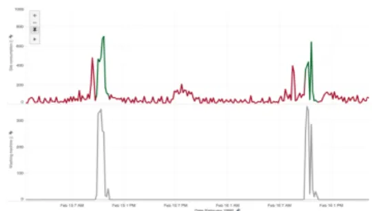
[25] for consumption readings at 15-minutes for houses in the Netherlands and training the model on benchmark Dutch houses using plugs. The results obtained from the data at these commonly observed sapling rates are then compared. In Fig. 3 the non-event based method is shown and the electrical-signature of a washing machine at 15-minutes.
III. DATABASEARCHITECTURE
The database is provided from Greeniant B.V, which is a smart meter analytics company based in the Netherlands. The database consists of more than three thousand residential customers with the corresponding meter reading hosted in cloud based server. The training of the proposed model is built on a subset of the Greeniant B.V database (approx. 20 houses) with plugs for various appliance reading. For the purpose of validation the technology, four new houses were selected with additional plugs for the appliance power reading were installed. The database corresponded to varying houses in terms of consumption level, number of inhabitants and area of the house. The results are the average for appliances across all the houses.
IV. METHODOLOGY
The methodology can be described as a part based data driven approach. The meter reading is a time series from which daily overlapping sub-sequences are generated. The time se-ries, sub-sequence and sliding time windows are described as follows:
Time Series: Ordered set of n real-valued variables T = t1, . . . , tn.
Sub-sequence: For a given time series T of length n, a sub-sequence Ck of T is a sampling of length
w ≤ n of contiguous position from T , that is, Ck=
tk, . . . , tk+(w−1) for 1 ≤ k ≤ n − (k + 1).
Sliding Time Window:Given a time series T of length n and a subsequence length of w, a matrix M of all possible subsequence can be built by “sliding time window” across T and placing subsequence Ck in
the kthrow of M . The size of matrix M is (n − k + 1)/n × w.
An appliance is identified to be used in a particular day if it starts before the end of the day (24:00). Four hours of additional time overlap at the end of the day is taken for the
cross-over cases. The raw training data consists of 10-seconds active power reading together with the energy consumption during the period. The 10-second active power reading is used for the 10-second analytics whereas the 15-minutes consumption reading is used for the 15-minutes analytics. A. 10-second analytics
The 10-second smart meter analytics consists of the follow-ing stages:
1) Preprocessing of the data.
2) Element generation from the ON/OFF events.
3) Appliance-wise filter parameter generation from training database. (Both smart meter and appliance data) 4) Element detection based on trained filter parameters 5) Calculation of start time and energy after appliance
detection.
1) Pre-processing: At the preprocessing stage the signal noise such as data spikes and outages are processed and removed.
It is important to remove the spikes as they interfere with element detection. The spikes are removed using a median filter. In the data received from the server if the outage in the data is above a pre-defined threshold then appliance identification during the period is not considered.
2) Element generation from the ON/OFF events: The event is registered when the change in power level is above 35 W. This minimum threshold is chosen to reduce event complexity and to reduce the error of minor fluctuations. In Fig. 4, low power fluctuation seen in some smart meter data is shown.
The delta calculation can be expressed by the following equation:
∇(ti) = P (ti) − P (ti− 1)
∇(ti) > 35W
)
ti∈ [0, w] (1)
where ‘w’ is the window size. In Fig. 5 the events generated for a typical 10 second smart meter reading is shown. It can be seen clearly that the generated events correspond to various appliance states. The blue color corresponds to ‘no appliance indentification’ and the other colors are for ‘detected appliances’.
Element generation: Within the time-window (experimen-tally set to four hours based on maximum appliance duration), a list of consecutive positive events are sorted, and a list
(a) NILM non-event based (generic).
(b) The 15-minutes smart-meter and washing machine consump-tion.
Fig. 3: Non-event based NILM, both generic and practical example.
Fig. 4: 32 W fluctuation in the meter-data.
Fig. 5: Events generated from the three consecutive use of washing machine (In red).
of consecutive negative events are sorted that come after the last positive. One negative event at a time is taken and subsequently matched with a positive event in the list of positive event. The events matched are removed and the process followed iteratively.
3) Appliance signature parameter calculation: Once the elements are generated the subsequent step is to generate its features or signature. The features are evaluated to consider the power levels, duration, number of occurrence and gaps within appliance states.
• Mean and Standard deviation of the ON and OFF duration in the window.
• Number of occurrences within the window.
• Mean and standard deviation of the power level.
• Time difference between the various appliance electrical elements.
As previously stated the power level based clustering roughly corresponds to various states or elements of a multi-state appliance and helps us to consider the temporal relation between the various states.
4) Training of part based model parameters: In Fig. 6 it can be seen how the grouped elements roughly can be interpreted as appliance states. Once the features are generated for each time-window, it becomes training instance for the classifier and all the training instances are generated using the sliding time window (typically window jump of 30-minutes). The output or appliance state is taken to be ON if the appliance is 100 % present in the time-window. Once, the training instances are generated, the task is to learn a classifier function which can best map the input to the output (appliance state).
Fig. 6: The generated elements relation to appliance states.
B. 15 minutes NILM
The 15-minutes load dis-aggregations algorithm is trained from the consumption reading at 15-minutes. The data is only pre-processed for outlier removal but no thresholding is performed.
1) The aggregate energy readings are extracted for the 20 houses at a sampling rate of 15 minutes.
2) Multiple sub-sequences and one class output are gener-ated from each data-set using temporal sliding window with a window size of 6 units.
3) The classifier is trained with the generated features as input attributes and high energy appliances as output classes [19].
4) The model is trained from the 20 houses for a period of 4-weeks.
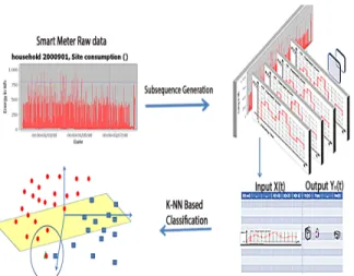
A simplified graphical work-flow of this approach is illus-trated in Fig. 7 from step one to four.
Fig. 7: Methodology: 15-minutes load disaggregation. The features generated step is implemented from the [19] article but the sampling rate are different.
V. RESULT
In this section, firstly, the measure used to evaluate the per-formance is discussed followed by the observed perper-formance metrics using two different sampling rates.
A. Measures
Given a dataset of labelled instances, supervised machine learning algorithms seek a hypothesis that will correctly pre-dict the class of future unlabelled instances. In order to com-pare structures of predictors, we need indicators that will give a quantitative way of assessing the classifier performances. While comparing these indicators values, the best predictor can be found for a given appliance.
In order to properly define the performance indices of the classification algorithms used for prediction, we introduce the confusion matrix [26].
A confusion matrix contains information about the actual and the predicted results obtained by a classification system. The performances of such systems are commonly evaluated using the data contained in this confusion matrix. Table I shows the confusion matrix for a two-class classifier. The classes that can be predicted are “positive” or “negative” instances, which in this case signifies the appliance consumes or does not consume energy.
TABLE I: Confusion matrix
Predicted Negative Positive
Actual Negative a b
Positive c d
In the context of this study, the entries defined in the con-fusion matrix reported in Table I have the following meaning: a : is the number of correct predictions where an
in-stance is negative,
b : is the number of incorrect predictions where an instance is positive,
c : is the number of incorrect of predictions where an instance negative,
d : is the number of correct predictions where an in-stance is positive.
Several standard terms have been defined for this 2 class matrix:
The true positive rate (recall): is the proportion of positive cases that were correctly identified, as calculated using the equation T P = d/(c + d). Represents the ratio between the predicted positives states of the appliances (ON) and the total number of correct positives states of the appliances.
The precision:is the proportion of the predicted pos-itive cases that were correct, as calculated using the equation P = d/(b + d). Represents the fraction of the positives states (ON) of the appliances correctly predicted.
A correct appliance identification is defined as being one where the start time is +/- thirty minutes of the actual start time and for the correct appliance. The false-positive impact for use-cases is much more than the impact of false-negative thereby the precision scores are presented.
B. Dis-aggregation performance
In Table II the appliance-wise dis-aggregation performance is shown for the major white goods appliances present in a typical Dutch residence. The washing machine is present in all the houses and the electric oven in just one as in most residence it is run on gas. It can be observed from the results that the performance is better for the washing machine and dish washer, it reduces significantly for the clothes dryer and particularly electric oven. In case of 15 minutes sampling rate, the washing machine and dish-washer are considerably reduced and are mostly detected during the non-peak times. The major cases of error are also the clothes drier vis-a-vis Oven error due to mis-labelling. This can be improved by taking context into account, e.g. a Drier is generally used after the washing machine.
TABLE II: Dis-aggregation performance, Precision (measure).
Sampling Rate Appliances
Washing Machine Clothes Drier Dish Washer Electric Oven 10 second .89 .64 .79 .50 15 minutes .5 .6 .5 .32 C. Discussion
The proposed method is an industrial application at 10-second and 15-minutes sampling showing the pros and cons
of using load dis-aggregation in residences. The existing literature is based on acquired dataset but not actual customers, which is a challenge in itself, addressed in this work. This method is an implementation of existing methods enhanced by the data-processing and a large training database. This work also emphasizes the gap between the trained models in a benchmark dataset and the intricacies of an application to actual people who have different appliances combinations and usages.
VI. CONCLUSION
NILM has acquired considerable amount of interest in the smart-energy domain and this work presents a comparison of results for two sampling rate for various appliances present in a typical house. It is observed that the performance is correlated to the number of appliances being present in the house as the signal of appliances other than the one which is being identified is considered noise.
The results also highlight the fact that performance of load dis-aggregation decrease as we move from the laboratory setting to the real residences. This may happen due to error at various stages; data acquisition, inter-appliance similarity, presence of previously unobserved appliances etcetera. The recording of household meta-data (appliances present in the house) could be used to reduce mis-labelling among appliances and thereby increase the performance. Finally, the results indicate that the proposed 10-second NILM algorithm is deployable for majority of houses (> 80 %) with a use case for the customer. In case of 15 minutes consumption data, the appliances detection are limited to the non-peak periods of the day.
VII. ACKNOWLEDGEMENT
This work has been a joint collaboration by the project PARADISE which is sponsored by the National Research Agency (ANR), France and the smart meter analytics enter-prise Greeniant B.V operating from the Netherlands.
REFERENCES
[1] T. Strasser, F. Andr´en, M. Merdan, and A. Prostejovsky, “Review of trends and challenges in smart grids: An automation point of view,” in Industrial Applications of Holonic and Multi-Agent Systems, ser. Lecture Notes in Computer Science. Springer Berlin Heidelberg, 2013, vol. 8062, pp. 1–12.
[2] P. Palensky and D. Dietrich, “Demand side management: Demand response, intelligent energy systems, and smart loads,” Industrial In-formatics, IEEE Transactions on, vol. 7, no. 3, pp. 381–388, 2011. [3] D. He, W. Lin, N. Liu, R. Harley, and T. Habetler, “Incorporating
non-intrusive load monitoring into building level demand response,” Smart Grid, IEEE Transactions on, vol. 4, no. 4, pp. 1870–1877, Dec 2013. [4] P. Siano, “Demand response and smart grids - a survey,” Renewable and
Sustainable Energy Reviews, vol. 30, no. 1, pp. 461–478, 2014. [5] K. Basu, L. Hawarah, N. Arghira, H. Joumaa, and S. Ploix, “A prediction
system for home appliance usage,” Energy and Buildings, vol. 67, no. 1, pp. 668–679, 2013.
[6] K. Basu, M. Guillame-Bert, H. Joumaa, S. Ploix, and J. Crowley, “Predicting home service demands from appliance usage data,” in Information and Communication Technologies and Applications (ICTA), International Conference on, 2011.
[7] B. Birt, G. Newsham, I. Beausoleil-Morrison, M. Armstrong, N. Sal-danha, and I. Rowlands, “Disaggregating categories of electrical energy end-use from whole-house hourly data,” Energy and Buildings, vol. 50, pp. 93–102, 2012.
[8] G. Hart, “Nonintrusive appliance load monitoring,” Proceedings of IEEE, vol. 80, no. 12, pp. 1870–1891, 1992.
[9] T. Hassan, F. Javed, and N. Arshad, “An empirical investigation of v-i trajectory based load sv-ignatures for non-v-intrusv-ive load monv-itorv-ing,” Smart Grid, IEEE Transactions on, vol. 5, no. 2, pp. 870–878, March 2014.
[10] M. Dong, P. Meira, W. Xu, and C. Chung, “Non-intrusive signature extraction for major residential loads,” Smart Grid, IEEE Transactions on, vol. 4, no. 3, pp. 1421–1430, Sept 2013.
[11] M. Zeifman and R. Kurt, “Nonintrusive appliance load monitoring: Review and outlook,” Consumer Electronics, IEEE Transactions on, vol. 57, no. 1, pp. 76–84, 2011.
[12] J. Li and N. Allinson, “Building recognition using local oriented features,” Industrial Informatics, IEEE Transactions on, vol. 9, no. 3, pp. 1697–1704, 2013.
[13] M. Berges, E. Goldman, H. Matthews, and L. Soibelman, “Enhancing electricity audits in residential buildings with nonintrusive load monitor-ing,” Journal of Industrial Ecology, vol. 14, no. 5, pp. 844–858, 2010. [14] T. Bier, D. Benyoucef, D. Abdeslam, J. Merckle, and P. Kleinf, “Smart meter systems measurements for the verification of the detection & classification algorithms,” in Industrial Electronics Society, IECON 2013-39th Annual Conference of the IEEE. IEEE, 2013, pp. 5000– 5005.
[15] R. Fernandes, I. da Silva, and M. Oleskovicz, “Load profile identification interface for consumer online monitoring purposes in smart grids,” Industrial Informatics, IEEE Transactions on, vol. 9, pp. 1507–1517, 2013.
[16] L. Norford and S. Leeb, “Non-intrusive electrical load monitoring in commercial buildings based on steady-state and transient load-detection algorithms,” Energy and Buildings, vol. 24, no. 1, pp. 51–64, 1996. [17] G. Kalogridis, C. Efthymiou, S. Denic, T. Lewis, and R. Cepeda,
“Pri-vacy for smart meters: Towards undetectable appliance load signatures,” in Smart Grid Communications (SmartGridComm), 2010 First IEEE International Conference on, oct. 2010, pp. 232–237.
[18] A. Prudenzi, “A neuron nets based procedure for identifying domestic appliances pattern-of-use from energy recordings at meter panel,” in Power Engineering Society Winter Meeting, 2002. IEEE, vol. 2, 2002, pp. 941–946.
[19] K. Basu, V. Debusschere, S. Bacha, U. Maulik, and S. Bondyopadhyay, “Nonintrusive load monitoring: A temporal multilabel classification approach,” Industrial Informatics, IEEE Transactions on, vol. 11, no. 1, pp. 262–270, Feb 2015.
[20] K. Basu, V. Debusschere, A. Douzal-Chouakria, and S. Bacha, “Time series distance-based methods for non-intrusive load monitoring in residential buildings,” Energy and Buildings, vol. 96, pp. 109 – 117, 2015. [Online]. Available: http://www.sciencedirect.com/science/article/ pii/S0378778815002133
[21] H. Ahmadi and J. Marti, “Load decomposition at smart meters level using eigenloads approach,” Power Systems, IEEE Transactions on, vol. 30, no. 6, pp. 3425–3436, Nov 2015.
[22] J. Kolter, S. Batra, and A. Ng, “Energy disaggregation via disciminative sparce coding,” Advances in Neural Information Processing Systems, vol. 23, no. 7, pp. 1153–1161, 2010.
[23] O. Parson, S. Ghosh, M. Weal, and A. Rogers, “Using hidden Markov models for iterative non-intrusive appliance monitoring,” in Neural Information Processing Systems workshop on Machine Learning for Sustainability, December 2011, event Dates: 17 December 2011. [Online]. Available: http://eprints.soton.ac.uk/272990/
[24] N. Henao, K. Agbossou, S. Kelouwani, Y. Dube, and M. Fournier, “Approach in nonintrusive type i load monitoring using subtractive clustering,” Smart Grid, IEEE Transactions on, vol. PP, no. 99, pp. 1–1, 2015.
[25] K. Basu, V. Debusschere, and S. Bacha, “Load identification from power recordings at meter panel in residential households,” in XXth International Conference on Electrical Machines (ICEM), September 2-5, Marseille, France, 2012.
[26] R. Kohavi and F. Provost, “Glossary of terms,” Editorial for the Special Issue on Applications of Machine Learning and the Knowledge Discovery Process, vol. 30, pp. 271–274, February 1998.