HAL Id: hal-01443817
https://hal.laas.fr/hal-01443817
Submitted on 23 Jan 2017
HAL is a multi-disciplinary open access
archive for the deposit and dissemination of
sci-entific research documents, whether they are
pub-lished or not. The documents may come from
teaching and research institutions in France or
abroad, or from public or private research centers.
L’archive ouverte pluridisciplinaire HAL, est
destinée au dépôt et à la diffusion de documents
scientifiques de niveau recherche, publiés ou non,
émanant des établissements d’enseignement et de
recherche français ou étrangers, des laboratoires
publics ou privés.
Constraint programming for planning test campaigns of
communications satellites
Emmanuel Hébrard, Marie-José Huguet, Daniel Veysseire, Ludivine
Boche-Sauvan, Bertrand Cabon
To cite this version:
Emmanuel Hébrard, Marie-José Huguet, Daniel Veysseire, Ludivine Boche-Sauvan, Bertrand Cabon.
Constraint programming for planning test campaigns of communications satellites.
Constraints,
Springer Verlag, 2017, 22 (1), pp.73 - 89. �10.1007/s10601-016-9254-x�. �hal-01443817�
Constraint Programming for Planning Test
Campaigns of Communications Satellites
Emmanuel Hebrard1, Marie-Jos´e Huguet1, Daniel Veysseire1, Ludivine Boche
Sauvan1,2, and Bertrand Cabon2
1
LAAS-CNRS, Universit´e de Toulouse, CNRS, INSA, Toulouse, France
2
Airbus Defence & Space, Toulouse, France
Abstract. The payload of communications satellites must go through a series of tests to assert their ability to survive in space. Each test involves some equipment of the payload to be active, which has an impact on the temperature of the payload. Sequencing these tests in a way that ensures the thermal stability of the payload and minimizes the overall duration of the test campaign is a very important objective for satellite manufacturers.
The problem can be decomposed in two sub-problems corresponding to two objectives: First, the number of distinct configurations necessary to run the tests must be minimized. This can be modeled as packing the tests into configurations, and we introduce a set of implied constraints to improve the lower bound of the model.
Second, tests must be sequenced so that the number of times an equip-ment unit has to be switched on or off is minimized. We model this aspect using the constraint Switch, where a buffer with limited capac-ity represents the currently active equipment units, and we introduce an improvement of the propagation algorithm for this constraint.
We then introduce a search strategy in which we sequentially solve the sub-problems (packing and sequencing). Experiments conducted on real and random instances show the respective interest of our contributions.
1
Introduction
The payload of a communications satellite is the on-board equipment that is actually relevant to the mission: receiving, amplifying and returning the signal. A set of tests are necessary to certify that the payload will correctly perform its mission. A test is characterized by a set of active equipment units and several thermal constraints limit the number of equipment units that can be made active simultaneously. The duration of the tests themselves is incompressible. However, activating some equipment takes time as each equipment unit much reach a given temperature and the temperature of the entire payload must be stabilized before tests can resume. Therefore, the total transition time depends on the order in which tests are sequenced. The goal is to sequence all the tests so that the overall duration is minimized.
Two main approaches have been previously considered. In the first approach [8], tests requiring the same subset of active equipment are packed together in the
same payload configuration. The transition time between tests run in the same configuration is null since no equipment activation is required. Between two con-figurations, however, some equipment units must be activated or deactivated and the heat of the payload must be stabilized before the next configuration, which entails important transition times. The objective of this approach is to minimize the number of configurations necessary for running all the tests. More-over, a secondary objective is to minimize the overall number of activations and deactivations since the time required to stabilize the temperature of the payload is correlated, though not linearly, to the number of simultaneous activations. In practice, the transition time between two configurations is considered as a constant value sufficient to stabilize the temperature in the payload. Maillet et al. [8] first proposed a constraint programming approach to address this problem, using backjumping and dedicated heuristics.
It is in principle possible to activate an equipment unit whilst tests on other units are being run. The second approach, presented in [2], relies on this idea. An equipment activation is viewed as a task with a given duration. If an equipment unit is not tested during a period equal to this duration and if the thermal constraints allow it, then it can be activated at the beginning of this period, and becomes available for other tests at the end. It may be possible to do so for several or even all equipment activations, thus effectively masking the transition times. A local search method (simulated annealing) was proposed in [2] for this second approach, that is, with “online” activation allowed. It was shown that this approach can reduce the overall duration of the test campaign. However, the total number of activations can be higher in some instances.
Finally, since the focus in [8] was on selecting a subset of tests to be run rather than sequencing them, a straightforward improvement of the first approach was proposed in [2]: Once every test is allocated to a configuration and the number of configurations is minimized, the problem of minimizing the number of activations between consecutive configurations can be seen as a Traveling Salesman Problem (TSP). As the number of configurations is typically small, this problem can be solved optimally even with relatively basic TSP methods.
The second approach is difficult to implement in practice as activations and deactivations can happen continuously, making the detailed thermal analysis of the process a difficult task, whereas thermal engineers only need to worry about transitions between configurations in the first approach. In this work, we present a study for Airbus, which currently only implements the first approach. We propose an improved constraint programming approach to solve the problem. Since thermal constraints limit the number of tests that can be run in the same configuration, this problem has a packing component, where tests have to be allocated to a minimum number of configurations. We introduce a set of implied constraints to improve the lower bound on this objective.
Moreover, this packing component is intertwined with a sequencing compo-nent where configurations must be ordered so that the number of equipment activations is minimized. We observe that this secondary objective can be eas-ily modeled using the constraint Switch [1]. This constraint models a resource
operating as a buffer of limited capacity and whose content can be changed, how-ever at a cost. Tests require equipment to be active and thermal constraints limit the number of simultaneously active equipment units, which can thus be seen as buffered. Moreover, the number of activations, which correspond to switches in the buffer, should be minimized. We introduce a simple improvement of the propagation algorithm for this constraint in the very common case where we have prior knowledge about the items that must be eventually buffered.
Next, we introduce a search strategy in which we sequentially solve the two sub-problems. We solve first the packing problem with a dedicated branching heuristic to find upper and lower bounds on this objective quickly. Then we solve a much simplified sequencing problem since tests are already allocated to configurations. This approach is not complete, and hence we must solve the over-all problem in order to find optimal solutions. However this is made significantly easier thanks to the upper and lower bounds found in the previous phases.
Finally, we experimentally evaluate the different contributions and assess the benefit of our method with respect to the current approach in use at Airbus.
2
Formal Background
A constraint satisfaction problem (CSP) consists of a set of variables, where each variable Xk has a finite domain of values D(Xk), and a set of constraints
specifying allowed combinations of values for subsets of variables. A solution of a CSP is an assignment of values to the variables satisfying the constraints.
We consider both integer and set variables. A set variable Yi is represented by its lower bound Yi which contains the required elements and an upper bound
Yiwhich contains the possible elements. For a finite universe U ⊂ N, we identify
a set variable Yi with the set of Boolean variables {Y j
i | j ∈ U }. The predicates
Yij = 1 and j ∈ Yi are equivalent, as are |Yi| = κ andPj∈eYij= κ.
For two integers a ≤ b, we denote [a, b] the set of consecutive integers {a, . . . , b}, and use the shortcut notation [b] for [1, b].
We shall often denote a sequence of variables or constants (c1, . . . , cn) by c
(where the length n is either recalled or clear from the context).
2.1 The constraints Switch and BufferedResource
The constraints Switch and BufferedResource [1] were introduced to model a type of resource corresponding to a buffer which must contain the items re-quired by some tasks when they are being processed. Such resources are limited in two ways: first, the buffer can only hold a limited number of items, and second, there is an upper bound on the number of item switches along the sequence.
In our context, these constraints are useful to model thermal constraints together with the objective to minimize the number of activations (switches) of equipment units (items to be buffered). The constraint Switch involves a sequence of set variables Y = (Y1, . . . , Yn) and an integer variable M. The set
variable M represents the total number of items that are removed from the buffer to make room for new items:Pn−1i=1 |Yi\ Yi+1|. Moreover, the buffer has
a minimum and maximum capacity (lower and upper bound on |Yi|) which are
allowed to be different at every position i. Let Y be a sequence of set variables, and κ, κ be two sequences of constants of same size n.
Definition 1 (Switch).
Switch(Y, κ, κ, M) ⇐⇒ ∀i ∈ [n], κi≤ |Yi| ≤ κi ∧ X
1≤i<n
|Yi+1\ Yi| ≤ M
Often, we know beforehand which tasks are to be performed and which items are required by each task. In this case, one can use the BufferedResource constraint which involves a sequence of integer variables X = (X1, . . . , Xn)
rep-resenting a permutation of n tasks, and a sequence t = (t1, . . . , tn) of sets of
integers standing for the items required by each task. Achieving arc consis-tency on this constraint is NP-hard, and there is no dedicated propagation al-gorithm for this constraint, besides the obvious decomposition using Switch, AllDifferent[12] and some Element [7] constraints.
Definition 2 (BufferedResource).
BufferedResource(X, Y, κ, κ, t, M) ⇐⇒ Switch(Y, κ, κ, M) ∧ ∀i < j ∈ [1, h], Xi6= Xj ∧
∀i, ti⊆ YXi
In our test planning problem, the buffers have equal upper and lower bounds. We shall therefore use a single integer parameter to denote the sequences κ and κ in the remainder of the paper.
3
Test Planning
3.1 Data and Constraints
A test campaign involves n tests and m equipment units. Every test k ∈ [n] involves a subset tk ⊆ [m] of equipment units to be active.1A payload
configu-ration (or simply configuconfigu-ration) is defined by a partition of the equipment into active and inactive units. A test k can occur in a configuration if the set of active equipment units in that configuration is a superset of tk.
However, one cannot use a single configuration where every equipment unit is active, because the payload would overheat. Equipment units that are on the same wall or blade of the satellite contribute to the overall temperature of that wall/blade. Therefore, we have p constraints, one for every set of equipment units
1
Throughout the paper, an equipment unit is said to be “active” if it is switched on and “inactive” otherwise.
whose thermal profiles are linked. For each thermal constraint ℓ ∈ [p], we define a subset cℓ⊆ [m] of size ∆ℓof equipment units, among which exactly2κℓshould
be active at the same time, i.e., in the same configuration.
3.2 Decisions and Objectives
A test plan with h∗ configurations is a mapping τ from tests to a set of
consec-utive integers [h∗] (without loss of generality, we assume that configurations are
numbered 1 to h∗), and a mapping σ from configurations to subsets of equipment
units such that the equipment units required to run a test are active when this test is run and every configuration satisfies all thermal constraints.
The main objective is to minimize the number of configurations |{τ (k) | k ∈ [n]}|, in order to reduce the transition time between tests, that is, the time spent in reconfiguring the payload.
Moreover it is important to take into account the total number of changes in the status of an equipment unit. Indeed, even though several equipment units can be switched on or off simultaneously, changing the status of more units requires a more careful analysis of the thermal dynamics of the system and is more likely to destabilize it. The second objective therefore is the total number of times an equipment unit is switched on besides the initial activation: Phi=1∗ (|σ(i) \ σ(i − 1)|) − m, where σ(0) is assumed to be empty.
Indeed, it is important to take into account the total number of changes in the status of the equipment. Even though several equipment units can be switched on or off simultaneously, changing the status of more units requires a more careful analysis of the thermal dynamics of the system and is more likely to destabilize it. In order to count the total number of times each equipment unit is switched from inactive to active and vice versa, we must decide the order in which the planned configurations will be visited. By convention, since configuration names are arbitrary, the tests allocated to configuration i are run at the i-th position. Therefore, the same mapping τ defines both the allocation of tests to configurations and the sequence in which tests will be run.
We consider here that the packing objective has higher priority than the sequencing objective and thus that they are lexicographically ordered.
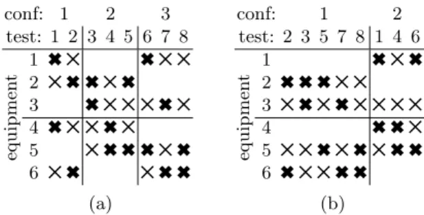
Example 1. Consider a set of 8 tests and 6 equipment units shown in Figure 1a. The equipment required by each test is indicated with the symbol 6. Moreover, assume that we have two thermal constraints with scopes c1 = {1, 2, 3} and
c2= {4, 5, 6} both of capacity 2.
The solution shown in Figure 1a (5 symbols indicate active equipment not involved in the current test) is suboptimal as it requires three configurations. Additionally, equipment units 1 and 6 must be activated twice.
However, with the permutation 2, 3, 5, 7, 8, 1, 4, 6 shown in Figure 1b, we only need two configurations and every equipment unit is activated exactly once.
2
Alternatively, one may only consider an upper bound only to prevent the system from overheating, however thermal engineers advise to keep the system as stable as possible, hence our choice of an equality.
conf: 1 2 3 test: 1 2 3 4 5 6 7 8 eq u ip m en t 1 6 52 5 6 6 5 66 5 5 3 6 5 5 5 6 5 4 6 5 5 6 5 5 5 6 6 6 5 6 6 5 6 5 6 6 (a) conf: 1 2 test: 2 3 5 7 8 1 4 6 eq u ip m en t 12 6 6 6 5 56 5 6 3 5 6 5 6 5 5 5 5 4 6 6 5 5 5 5 6 5 6 5 6 6 6 6 5 5 6 6 (b)
Fig. 1: A solution with 3 configurations and 2 extra activations (1a), and an optimal solution with 2 configurations and no extra activation (1b).
3.3 Complexity
It is relatively easy to see that the test planning problem described above is NP-hard. We show that the decision version TestPlanning, which asks whether there exists a plan with at most h configurations is NP-complete.
Theorem 1. TestPlanning is NP-complete.
Proof. It is in NP since a plan can be checked in polynomial time.
To prove hardness, we use a straightforward reduction from 3-coloring, which asks, given a graph G = (V, E), whether there exists a coloring of V with at most 3 colors such that no edge has its two end points of the same color.
From a graph G = (V, E), we build an instance of TestPlanning as follows: – For every edge (x, y) ∈ E, there are two equipment units xy and yx and a
thermal constraint on these two units with capacity 1.
– For every vertex x ∈ V we create a test txinvolving equipment units xy for
every y such that (x, y) ∈ E.
It is easy to see that two tests txand ty can share the same configuration if
and only if there is no edge (x, y) ∈ E. Therefore, G has a 3-coloring if and only if there is a plan with at most 3 configurations, and hence TestPlanning is
NP-hard for h = 3. ⊓⊔
Moreover, even if we let the number of configurations free, minimizing the number of switches is also NP-hard for a single thermal constraint over all equip-ment of capacity κ since it corresponds exactly to the constraint:
BufferedResource(X, Y, κ, t, M)
where X (resp. Y) is a sequence of n integer (resp. set) variables, and for every k ∈ [n] the variable Xk has domain [n] and the variable Yk ranges between the
The number of simultaneously active equipment units must be equal to κℓ,
therefore, we can consider actived equipment as a buffer of capacity exactly κℓ.
Moreover, the set of equipment units tk required by a test k corresponds to
the items required to be in the buffer when processing this task. Finally, the objective is to minimize the number activations which is equivalent, up to a constant, to the number of switches M. The reduction from Hamiltonian path to BufferedResource provided in [1] can be lifted to this particular case.
4
A Constraint Model for Test Planning
Let h ≤ n be some known upper bound on the number of configurations. We use n allocation variables {Xk | k ∈ [n]} with domain [h] standing for the
configuration allocated to each test. Unless we have a valid upper bound, the maximum number of configurations h is equal to n. Next, we use m × h activity variables {Yij | j ∈ [m], i ∈ [h]} standing for the status of equipment unit j in configuration i, i.e., Yijis equal to 1 if unit j in switched ON in i and is equal to 0 otherwise. Moreover, we denote YU
i the set variable with characteristic function
{Yij| j ∈ U }. For instance, Yi[m]has as characteristic function the set of variables in the column i of the m × h matrix formed by the activity variables, i.e., the set of equipment units active in configuration i. We introduce a variable Mℓfor each
constraint ℓ standing for the total number of switches on the equipment units cℓ. Finally, we have two variables to express the objective function: a variable N
standing for the number of configurations and a variable M for the total number of switches.
To model the test planning problem, we then post the following constraints:
∀k ∈ [n], tk⊆ Y [m] Xk (1) ∀ℓ ∈ [p], ∀i ∈ [h], |Ycℓ i | = κℓ (2) ∀k ∈ [n], N ≥ Xk (3) ∀ℓ ∈ [p], Switch(Ycℓ, κ ℓ, Mℓ) + κℓ− ∆ℓ (4) M =Ppℓ=1Mℓ (5)
Constraints (1) channel the allocation variables and the activity variables to ensure that every equipment unit required by a test is active in the slot in which the test is ran. They are implemented as Element constraints.
Constraints (2) enforce the thermal constraints on the number of equipment units active simultaneously within given subsets. They are implemented as sim-ple Sum constraints.
Constraints (3) ensure that the variable representing the number of config-urations is greater than or equal than the maximum allocated slot. We do not use a Maximum constraint nor an equality as we minimize this criterion.
Constraints (4) count the number of switches in the sequence of set vari-ables Ycℓ = (Ycℓ
1 , . . . , Y cℓ
h ) for every thermal constraint ℓ. The Switch
Ph
i=1|Yicℓ\Yi+1cℓ | = Mℓ, for a capacity κℓof the buffer. The constant term κℓ−∆ℓ
is used to count only from the second activation of each equipment unit. The constraint Switch counts the number of deactivations. Moreover, the κℓ items
contained in the buffer at the last position are not counted by Switch, even though they will eventually be switched off. The total number of deactivations is thus Mℓ+ κℓ and it is equal to the number of activations. Then each of the
∆ℓequipment units constrained by ℓ must be activated at least once, so we can
subtract this number to obtain the number of activation besides the first. Finally, Constraint (5) computes the overall sum of switches.
We consider the number of configurations as a higher priority objective than the total number of switches. Therefore, we express the objective function to minimize as the weighted sum (mh/2)N + M.
The Test Planning problem may be decomposed into two sub-problems: – a Test Packing problem when restricting to Constraints (1), (2) and (3) and
the minimization of the number of configurations N ;
– a Test Sequencing problem when restricting to Constraints (1), (4) and (5) and the minimization of the total number of switches M.
For the type of satellites we have considered in this study, there is no overlap in the scope of thermal constraints since they stand for the physical support of a disjoint subset of equipment units. However, overlaps may exist in some satellite architectures. In this case, we need to replace the constraints (4) and (5) by a single Switch constraint on the sequence of set variables Ym= (Y[m]
1 , . . . , Y [m] h ): Switch(Y[m], p X ℓ=1 κℓ, M) (6)
5
Lower Bound for Test Packing
The problem restricted to Constraints (1), (2) and (3) has some similarities with the multi-dimensional bin packing problem [5]. Instead of a one dimen-sional capacity, the bins have a capacity κℓ for each of the p dimension/thermal
constraint. Moreover, for a test k requiring a set of equipment units tk, we can
compute a p-vector representing its weight in each of these dimensions. However, the weights are not additive since every equipment unit is activated at most once per configuration, irrespective of the number of tests requiring it in this config-uration. As discussed previously, it can also be seen as a coloring problem. The particular case where each test is on a single equipment unit could be seen as a generalization of list coloring to hypergraphs, as thermal constraints can be mapped to hyperedges. However, to our knowledge, there is no known method for this specific problem.
We therefore use a simple lower bound on the number of configurations based on the “capacity” of the thermal constraints. Indeed, if a thermal constraint ℓ
ensures that at most κℓ equipment units are active in a given configuration, and
if the tests involve ∆ℓ units, then at least ⌈∆ℓ/κℓ⌉ configurations are needed.
More generally, suppose that we have a lower bound Kjon the number of
config-urations in which an equipment unit j will be active. Given a thermal constraint ℓ, the sum of these lower bounds over all equipment units in cℓcannot be greater
than the number of configurations multiplied by the capacity κℓ, in other words,
for any constraint ℓ,l(Pj∈cℓKj)/κℓ
m
is a valid lower bound for N .
Now, consider an equipment unit j, and let Γj = {j′ | ∃k s.t. {j, j′} ⊆ tk}
be its “neighborhood”, that is, the set of units that will necessarily be active when running the tests requiring j. It might not be possible to activate all these equipment units within a single configuration because of the thermal constraints. More generally, the equipment unit j must be active in at least as many config-urations as are required to visit Γj, i.e., Kj ≥ max({
l|Γ
j∩cℓ|
κℓ
m
| ℓ ∈ [p]}), let Γj
be this lower bound.
The following two implied constraints enforce this lower bound:
∀j ∈ [m], Kj= max(Γj,Phi=1Y j i ) (7) ∀ℓ ∈ [p], N ≥l P j∈cℓKj κℓ m (8) However, Constraints 2 in the base model force every set variable Ycℓ
i to
have cardinality κℓ, even if no test is allocated to configuration i. In this case,
the configuration i would be a copy of configuration N since it satisfies every constraint and minimize the number of switches. However, this is not compatible with Constraint 7 since equipment units active in “dummy” configurations would still be counted. We therefore replace Constraints 2 with the following constraints on ph extra Boolean variables {Zℓ
i | i ∈ [h], ℓ ∈ [p]}: ∀ℓ ∈ [p], ∀i ∈ [h], Zℓ i ⇐⇒ P j∈cℓY j i > 1 (9) ∀ℓ ∈ [p], ∀i ∈ [h], Pj∈cℓYij = Zℓ i × κℓ (10) ∀ℓ ∈ [p], ∀i ∈ [h], N ≥ i ⇐⇒ Zℓ i (11)
Constraints 9 ensure that Zℓ
i equals 1 iff at least one equipment unit
con-strained by ℓ is active in configuration i. Constraints 10 ensure that, for every configuration i, either there is no active equipment (i is a dummy configuration) or exactly κℓfor every thermal constraint ℓ. Finally, Constraints 11 channel these
extra variables with the objective variable N by ensuring that (Zℓ
1, . . . , Zhℓ) is its
unary order encoding [13]. These constraints are necessary to obtain a filtering as strong as in the base model, while improving the lower bound on N .
6
Test Sequencing
The problem of minimizing the number of equipment activations can be naturally represented using the Switch constraint, since, as shown in Section 4, thermal
constraints and the fact that tests require some equipment units to be active can be modeled as buffered resources. Moreover, as often in problems that can be represented with a buffered resource, we know beforehand the set of items (here equipment units) that will be activated at least once. In other words, the total number of items to be buffered minus the capacity κℓ of the buffer is a
trivial lower bound on the required number of switches. However, the constraint Switchdoes not take this information into account and hence is “suboptimal”, especially when only a few tests have been allocated a configuration.
In this section, we propose an improvement of the propagator for Switch for the very common case where we have prior knowledge on a set of items that must eventually be buffered. In some cases, we can simply add the number of non-buffered items to the lower bound computed by the algorithm for Switch. However, this is not always true. We define a correct lower bound based on this idea in Theorem 2.
We define the variant Switch+ of the Switch constraint with an extra
parameter V indicating the items that must be put in the buffer at some point in the sequence. Let V be a set of integers, M an integer variable, Y = (Y1, . . . , Yn)
be a sequence of set variables, and κ, κ be two sequences of n integers. Definition 3. Switch+(Y, κ, κ, V, M) ⇐⇒ ∀i ∈ [n], κi≤ |Yi| ≤ κi ∧ X 1≤i<n |Yi+1\ Yi| ≤ M ∧ n [ i=1 Yi= V
We next recall some background about the constraint and in particular its propagation algorithm in Definitions 4 and 5. It is possible to find an optimal buffer sequence σ, that is, an assignment of Y that minimizes the value of M with the greedy procedure FindSupport introduced by [1] (Algorithm 1 in [1]). This algorithm explores the sequence once while maintaining all items in a list ordered by a priority relation ≺ based on two indices (nexti
∈(j) and nexti6∈(j))
for each item j. Definition 4. nexti
∈(j) is the least index i′≥ i such that j ∈ Yi′ if it exists and
n + 2 otherwise. nexti
6∈(j) is the least index i′ ≥ i such that j 6∈ Yi′ if it exists
and n + 1 otherwise.
The priority relation ≺ between two items is defined by the following criteria: Definition 5. At index i, and given two items j1< j2, we have j1≺ j2 if:
1. nexti
∈(j1) < nexti6∈(j1) and nexti∈(j1) ≤ nexti∈(j2), or
2. nexti
∈(j2) > nexti6∈(j2) and nexti6∈(j1) ≥ nexti6∈(j2)
and j2≺ j1 otherwise.
The procedure starts with σ(0) = ∅ and when moving to index i, it first adds all required items (i.e., in Yi) and removes all impossible items (i.e., not in Yi),
which yields the set σ(i) = Yi∩ σ(i − 1) ∪ Yi. If |σ(i)| > κi it then removes the
κi− |σ(i)| last items for the order ≺ in σ(i). Otherwise, if |σ(i)| < κiit adds the
κi− |σ(i)| first items for the order ≺ in Yi\ σ(i).
Definition 6. A stretch of a buffer sequence σ is a triple hj, a, bi such that the value j is buffered in σ during the interval [a, b] and j is not buffered at a − 1 nor at b + 1 (we assume that no item is buffered at 0 or n + 1). We say that a stretch hj, a, bi is optional if there is no i ∈ [a, b] such that j ∈ Yi. We say that
the item j is optional if there exists a stretch hj, a, bi and for all i ∈ [n], j 6∈ Yi.
Every stretch entails one switch, except if it extends until the end of the sequence. Therefore, if κ is the cardinality of the buffer at the last index of the sequence, the following observation holds:
Observation 1 A solution with α switches has κ + α stretches.
Lemma 1. If σ and σ′ are two buffer sequences found by FindSupport on two instances I and I′ equal on every index except one for which the lower
bound of the buffer at this index contains a single additional item j in I′, then
∀i ∈ [n], σ′(i) \ σ(i) ⊆ {j}.
Proof. An item not in the buffer at index i − 1 is added at index i only if: 1. the item is the lower bound Yi or
2. κi> |Yi∩ σ(i − 1) ∪ Yi| and it is in the |Yi∩ σ(i − 1) ∪ Yi| − κi first for ≺.
Only item j can satisfies case 1 in I′ but not in I.
Moreover, by definition, the order ≺ is equal in I and I′, except for j which
may be ranked higher in I′. Therefore, the only item that may satisfy case 2 in
I′ but not in I is again j. Therefore, ∀i ∈ [n], σ′(i) \ σ(i) ⊆ {j}. ⊓⊔
Lemma 2. Let σ be a buffer sequence of an instance I with minimal number of switches and let j be an item not buffered in σ. For any i ∈ [n], a sequence σ′ on the instance I′ obtained by adding the constraint j ∈ Y
i has at least one more
non-optional stretch than σ.
Proof. We can assume that σ and σ′ were found by FindSupport as this
al-gorithm is complete. The sequence σ′ has necessarily a non-optional stretch
hj, a, bi, and there was no j-stretch in σ. Therefore, if the number of non-optional stretches is not larger in σ′ than in σ, it must have one less non-optional j′
-stretch for an item j′ 6= j. This can only happen if the gap between two
non-optional stretches hj′, a
1, b1i and hj′, a2, b2i with b1+ 1 < a2is bridged by
buffer-ing the value j′ in the interval [b
1+ 1, a2− 1]. Hence there exists i such that
j′∈ σ′(i) \ σ(i). However, by Lemma 1 we have ∀i ∈ [n], σ′(i) \ σ(i) ⊆ {j}. ⊓⊔
Theorem 2. For any two sets V ⊆ U , if there is an optimal buffer sequence visiting exactly the items in U \ V with α switches, β optional stretches, and γ optional items, then there is no buffer sequence visiting all items in U in less than α + |V | − β + γ switches.
Proof. First, notice that we can reduce the case with γ > 0 optional items to the case without optional item, and β − γ optional stretches. Indeed, if there exists an optimal sequence σ visiting all items in U , we can add a constraint j ∈ Yifor
every pair (i, j) where j ∈ U and j ∈ σ(i). The procedure FindSupport will then find a sequence with same number of switches, same number of stretches, and γ less optional stretches than σ. Therefore, we suppose γ = 0 and prove the lower bound α + |V | − β.
Now, if σ has κ + α − β non-optional stretches, then by Lemma 2, we know that a solution visiting all items in U must have at least κ + α + |V | − β (non-optional) stretches, and hence at least α + |V | − β switches. ⊓⊔ Counting the number of optional stretches and items in the sequence returned by FindSupport can be done in linear time. Therefore, Theorem 2 improves the lower bound found by this algorithm without changing its worst case complexity when we know that some items must be buffered but do not appear in the lower bound of a set variable. This is true in the test sequencing problem, as it is in most applications of this constraint.
7
Search Strategy
In this section we introduce a dedicated branching heuristic for the packing problem. The basic idea is that we can easily evaluate the impact of allocating a test to a configuration by counting how many equipment activations are required and how these equipment units are already constrained in this configuration. Second, we propose to decompose the problem into packing and sequencing aspects in order to find good upper bounds quickly for the test planning problem.
7.1 Branching Heuristic Let δℓ
k(i) be the number of equipment units constrained by ℓ that will be active
in configuration i if test k was to be run in that configuration, i.e., the num-ber of non-ground Boolean activation variables concerning equipment of test k constrained by ℓ: δℓ k(i) = X j∈cℓ∩tk Yi j − Yji
We consider the ratio∆ℓ
κℓ to be proportional to the tightness of the constraint
ℓ, and we use the change in tightness resulting from the decision of running test k in configuration i to evaluate the impact of this decision. After the decision Xk = i, the tightness rb = ∆κℓℓ becomes ra = ∆ℓ−δ
ℓ
k(i)
κℓ−δkℓ(i)
. Therefore, the factor ra/rbrepresents the factor by which the tightness of constraint ℓ would increase.
As ra/rb ∈ [1, ∞], we use 1 minus its inverse as a measure, in [0, 1], of the impact
of that decision, that is:
γkℓ(i) = 1 −
∆ℓ(κℓ− δℓk(i))
Now, we can use the average of these impacts on all thermal constraints to define the impact γ(Xk← i) of allocating test k to configuration i.
γ(Xk← i) =
P
ℓ∈[p]γkℓ(i)
p
Notice that allocation variables may have many more values than necessary to satisfy the thermal constraints. Indeed, it is important, for a coloring heuristic, to branch only values in [i+1] where i is the highest allocated value so far. Hence, given a test k we consider the intersection bD(k) = D(Xk) ∩ [i + 1] instead of its
actual domain D(Xk). We therefore select the variable Xk minimizing:
| bD(k)| P
i∈ bD(k)γ(Xk← i)
And we branch on the value i minimizing γℓ k(i).
7.2 Multi-stage Approach
We use mh Boolean variables to represent the status of every equipment unit in every configuration. Moreover, without an upper bound on the number of con-figurations required to pack every test, we can only assume that n concon-figurations (as many as there are tests) may be needed, i.e., h = n. However, in practice n is a gross overestimate of h. For instance, in one of the industrial instances that we considered, several hundreds of tests can be run in as few as three configurations. Furthermore, since we consider two criteria in a hierarchical way, it makes sense to optimize a relaxation of the problem where only Constraints 1 to 3 are kept (the packing sub-problem), i.e., the model is complete with respect to the objective with highest priority. Observe that since the order of the bins does not matter in this case, configurations are symmetric. We therefore used lexicographic ordering constraints [4, 6] on the set variables Y1, . . . , Yh.
Last, we also considered the pure sequencing aspect of the problem. Given a packing, finding the optimal sequence for that packing can be modeled with a set of BufferedResource constraints, one for each thermal constraint, all sharing the same permutation. Another way to understand this is that we can consider a packing solution using h configurations as a new instance with only h tests to sequence (it is unlikely that two such tests could share a single configu-ration given the thermal constraints) and consider Constraints 1, 4 and 5 of the complete model (the sequencing sub-problem). Solving this problem to optimal-ity does not give us a lower bound on the total number of switches, however, it is much simpler and can often provide a good upper bound quickly.
We therefore implemented the following four-phase strategy:
1. We run a greedy descent on the packing problem to find an initial upper bound. The trivial heuristic that branch on the lexicographically least con-figuration for a test gives relatively good results, so we stop this phase at the first solution found, which is backtrack-free.
2. We run the packing model (initialized with the previous upper bound) for a given period of time, or until optimality is proven.
3. We run the sequencing model for a given period of time, or until optimality is proven (though in this case we cannot deduce a lower bound).
4. We run the complete model (packing & sequencing) (initialized with lower and/or upper bounds, accordingly) for the rest of the allocated time.
8
Experimental Evaluation
We tested the different approaches that we propose on industrial and gener-ated instances. We have only six real instances, corresponding to three already launched communications satellites. The same tests are usually run in two types of thermal environments. The hot and cold test phases respectively simu-late the periods where the satellite is facing the sun, or when it is in Earth’s shadow. Instances labeled cold are much more thermally constrained and thus typically require more configurations than those labeled hot. We diversified the pool of instances by randomly shuffling tests in order to produce 5 random-ized variants of every instance. Moreover, we used random instances designed to be similar to the real cases, generated as follows: for a given number of tests n ∈ {30, 50, 80, 100, 200, 300}, we set the number of equipment units to n/4. The equipment of instances with 30 and 50 tests are equally partitioned into 3 ther-mal constraints. Each test requires 2 equipment units from two different therther-mal constraints. Other instances have 5 thermal constraints and each test requires 2 or 3 equipment units belonging to different thermal constraints. Then, for each generated instance, we consider two levels of tightness for thermal constraints to simulate the hot (κℓ/∆ℓ =0.6) and the cold phases (κℓ/∆ℓ =0.4).
We generated 5 variants of 12 classes of instances. Instance XXX.YY denote a set of XXX tests with YY giving the ratio κℓ/∆ℓ of the thermal constraints.
Instances A, B and C are industrial instances. All models have been implemented in Choco 3 [10] and ran on Intel Xeon E5 processors for a total of thirty minutes on every instance. We compared the five following approaches:
– base is the straightforward model with Constraints 1 to 5, using Weighted Degree [3] for variable selection and lexicographic branching. Notice that the strategy is set up to branch on all allocation variables before branching on activity variables. Other predefined heuristics in Choco were less efficient. It is important to note that due to the “coloring” aspect of the problem, branching on the lexicographically least value (color) in the domain is ex-tremely important. However Impact Based Search [11] and Activity Based Search [9] cannot trivially be made to branch on the lexicographically least value and thus gave extremely poor results for that reason.
– heuristic is the same model as base, however with the dedicated heuristic described in Section 7.1 for variable ordering.
– multi-stage is the same model as base, however, using the four-phase strat-egy described in Section 7.2.
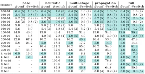
Table 1: Methods comparison. Average number of configurations and switches on random and industrial instances.
instance base heuristic multi-stage propagation full #conf #switch #conf #switch #conf #switch #conf #switch #conf #switch 030·04 6.4 (5) 1.6 (5) 6.4 (5) 1.6 (5) 6.4 (5) 1.6 (4) 6.4 (5) 1.6 (5) 6.4 (5) 1.6 (4) 030·06 3.4 (5) 0.8 (5) 3.4 (5) 0.8 (5) 3.4 (5) 0.8 (3) 3.4 (5) 0.8 (5) 3.4 (5) 0.8 (2) 050·04 5.2 (2) 2.2 (2) 5.2 (3) 2.0 (3) 5.2 (5) 2.0 (3) 5.2 (5) 2.0 (5) 5.2 (5) 2.0 (5) 050·06 3.6 (2) 0.8 (2) 3.6 (5) 0.6 (5) 3.6 (5) 0.6 (3) 3.6 (5) 0.6 (5) 3.6 (5) 0.6 (2) 080·04 9.6 19.0 9.0 (1) 15.0 (1) 9.0 15.4 9.0 (1) 13.8 (1) 9.0 (3) 13.8 (1) 080·06 5.6 6.0 5.4 (3) 4.8 (3) 5.4 (3) 5.2 (1) 5.4 (3) 4.2 (3) 5.4 (4) 4.2 (3) 100·04 14.0 40.6 13.0 43.4 13.2 31.8 13.0 34.4 12.8 30.2 100·06 4.4 5.8 4.0 (4) 2.8 (4) 4.0 (5) 4.0 4.0 (4) 3.0 (4) 4.0 (5) 2.8 (5) 200·04 12.6 67.2 10.2 62.8 10.2 46.2 10.4 53.6 10.0 47.8 200·06 5.8 24.2 5.0 18.2 5.0 17.2 5.0 14.0 5.0 14.4 300·04 - - 10.4 111.2 10.2 85.0 10.2 94.0 10.0 81.8 300·06 5.7 45.3 4.8 37.0 4.6 26.8 4.2 25.4 4.0 22.4 A cold 6.0 16.0 6.0 14.2 6.0 8.8 6.0 9.6 6.0 7.0 A hot 4.0 2.0 4.0 4.6 4.0 2.0 4.0 2.0 4.0 (5) 2.0 B cold - - 9.0 106.6 9.0 50.2 9.0 78.8 9.0 50.2 B hot - - 4.0 19.6 4.0 3.6 4.0 1.2 4.0 (5) 0.8 (2) C cold - - 8.0 82.8 8.0 46.8 8.0 64.8 8.0 50.6 C hot - - 3.0 15.0 3.0 2.0 3.0 (4) 0.2 (4) 3.0 (5) 0.0 (5)
– propagation augments the model base with symmetry breaking, the lower bound on the packing defined by Constraints (7) to (11), and the improve-ment on the propagator for Switch described in Section 6.
– full is the same model as propagation, however it uses the four-phases strategy and the branching heuristic described in Section 7.
Note that for every approach, we first applied a preprocessing to the data in order to merge identical tests. Indeed, on top of the packing based on the configuration of active equipment units, one must, in the real setting, further partition the tests because of different requirements on signal routing equipment. This second packing phase is exactly a list-coloring problem on the tests of each the configurations. The size of these problems is very modest with respect to state of the art coloring algorithms, so we do not study this aspect in the current paper. As a consequence, some tests in the data require the same set of equipment units to be active, and can be thought of as a single test for our purpose.
The results are reported in Table 1. For each method, we show the objective values, where #conf stands for the average number of configurations over the five variants of the instance, and #switch stands for the average number of switches for the same instances. Next to these values, we report in brackets, the number of instances for which the reported objective value was proven optimal within a 30 minutes time limit (no value means that none of the runs was complete). For each instance, the methods proving optimality in the most cases, among those giving the minimum average objective value, are color-highlighted.
First, we observe that the straightforward model base is very poor, in most of the larger instances it does not even find a feasible solution in less than ten minutes. On the other hand, augmenting this model either with stronger
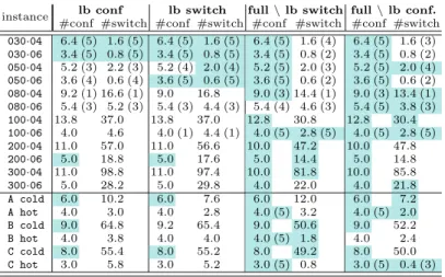
Table 2: Impact of the lower bounds. Average number of configurations and switches on random and industrial instances.
instance lb conf lb switch full\ lb switch full \ lb conf. #conf #switch #conf #switch #conf #switch #conf #switch 030·04 6.4 (5) 1.6 (5) 6.4 (5) 1.6 (5) 6.4 (5) 1.6 (4) 6.4 (5) 1.6 (3) 030·06 3.4 (5) 0.8 (5) 3.4 (5) 0.8 (5) 3.4 (5) 0.8 (2) 3.4 (5) 0.8 (2) 050·04 5.2 (3) 2.2 (3) 5.2 (4) 2.0 (4) 5.2 (5) 2.0 (3) 5.2 (5) 2.0 (4) 050·06 3.6 (4) 0.6 (4) 3.6 (5) 0.6 (5) 3.6 (5) 0.6 (2) 3.6 (5) 0.6 (2) 080·04 9.2 (1) 16.6 (1) 9.0 16.8 9.0 (3) 14.4 (1) 9.0 (3) 13.4 (1) 080·06 5.4 (3) 5.2 (3) 5.4 (3) 4.4 (3) 5.4 (4) 4.6 (3) 5.4 (5) 3.8 (3) 100·04 13.8 37.0 13.8 37.0 12.8 30.8 12.8 30.4 100·06 4.0 4.6 4.0 (1) 4.4 (1) 4.0 (5) 2.8 (5) 4.0 (5) 2.8 (5) 200·04 11.0 57.0 11.0 56.6 10.0 47.2 10.0 47.8 200·06 5.0 18.8 5.0 17.6 5.0 14.4 5.0 14.8 300·04 11.0 98.8 11.0 97.4 10.0 81.8 10.0 85.8 300·06 5.0 28.2 5.0 29.8 4.0 22.0 4.0 21.8 A cold 6.0 10.2 6.0 7.6 6.0 12.0 6.0 7.2 A hot 4.0 3.0 4.0 2.8 4.0 (5) 3.2 4.0 (5) 2.0 B cold 9.0 64.8 9.2 65.4 9.0 50.6 9.0 52.2 B hot 4.0 3.8 4.0 4.0 4.0 (5) 1.8 4.0 2.4 C cold 8.0 55.4 8.0 55.2 8.0 49.2 8.0 50.0 C hot 3.0 5.8 3.0 5.2 3.0 (5) 0.8 3.0 (5) 0.4 (3)
propagation, better branching heuristic, or the multi-stage approach is sufficient to obtain decent results. Combining all these improvements clearly yields the best and most robust results, and sometimes allows to prove optimality even on real industrial instances.
Second, multi-stage approaches (multi-stage and full) are clearly better for larger instances, however, they tend to hinder the ability of Choco to prove optimality on small instances. Moreover, we observed that they tend to be less robust, in the sense that the final result greatly depends on the initial packing which gives no guarantees on the number of switches. This is especially true for large instances in which the complete model often cannot improve on the heuristic sequence found during the third phase.
For a deeper analysis of the two bounds proposed in this paper, we ran four other models on the same instances. The first two are the base model augmented with the lower bound on configurations or the lower bound on switches (base ⊕ lb conf and base ⊕ lb switch, respectively). The other two models are the full model from which we removed these lower bounds (full \ lb switch and full \ lb conf , respectively). The results of these additional tests, in Table 2 clearly show that both bounds are useful. Surprisingly, the capacity to prove optimality on a criterion is also impacted by the bound on the other criterion.
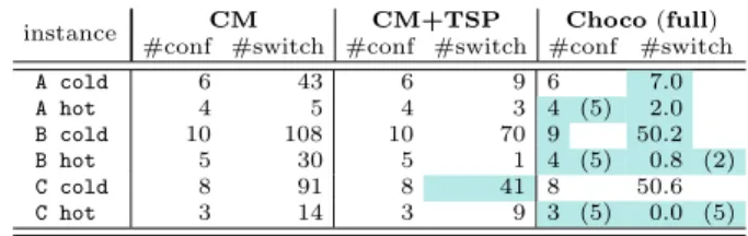
Finally, in Table 3, we compare the results of our best method (model full) with the method previously used by Airbus Defense & Space [8] and with a slight improvement of this method described in [2]. The former, denoted CM, is a con-straint optimization tool build to solve the packing problem only. The second, denoted CM+TSP, is the same approach, however the resulting configurations
Table 3: Comparison with current methods. Number of configurations and switches on industrial instances.
instance CM CM+TSP Choco(full) #conf #switch #conf #switch #conf #switch A cold 6 43 6 9 6 7.0 A hot 4 5 4 3 4 (5) 2.0 B cold 10 108 10 70 9 50.2 B hot 5 30 5 1 4 (5) 0.8 (2) C cold 8 91 8 41 8 50.6 C hot 3 14 3 9 3 (5) 0.0 (5)
are then permuted so that the Traveling Salesman Problem defined by the Ham-ming distance between configurations is optimized. It is not surprising that the first method is very poor in terms of total equipment activation since it makes no attempt to optimize this criterion. However, it is interesting to compare with our results as it is still the method used in practice.
The method CM+TSP gives a better solution in one case (C cold). Indeed, this instance is particular as it involves more than twice as many tests as other instances. The consequence is that the model computing packing and sequenc-ing simultaneously is relatively inefficient. For this instance, we therefore ran a simple randomized sequence of the second and third phases of the multi-stage approach (i.e., pure packing followed by pure sequencing) and quickly found a similar solution (though we could not improve on it). Notice that in the case of the “hot” test campaign for satellite C, carefully packing and sequencing the tests makes it possible to get rid of all equipment activation besides the mandatory one, whereas 14 activations are necessary with the current method.
9
Conclusion
We have introduced a complete constraint programming approach for the prob-lem of packing and sequencing the validation tests of communications satellites. We proposed a search strategy and lower bound for the packing aspect of the problem. Moreover, we introduced an improvement of the Switch constraint that can be applied in many other contexts. Our experimental evaluation shows that the methods proposed in this paper greatly improve the test plans with respect to those currently used within the Airbus group.
Although this approach is not yet industrially implemented, a previous in-ternal study in Airbus3 has shown that, during a test campaign, around 30% of
the total duration is spent on transitions between configurations. Moreover, in many cases, tests must be interrupted because the payload is overheating and
3
Master’s internship report by Ludivine Boche-Sauvan for the “Institut Sup´erieur de l’Aeronautique et de l’Espace” (ISAE) in 2012
can only resume after the system has been stabilized. The constraint model we introduced should help with both of these issues.
Since such test campaigns require an extremely costly and energy greedy thermal vacuum chamber as well as a large team of engineers in 3-shift rosters, significant financial savings are expected from this approach.
References
1. Christian Bessiere, Emmanuel Hebrard, Marc-Andr´e M´enard, Claude-Guy Quim-per, and Toby Walsh. Buffered resource constraint: Algorithms and complexity. In Proceedings of the Eleventh International Conference on Integration of AI and OR Techniques in Constraint Programming (CPAIOR), pages 318–333, 2014. 2. Ludivine Boche-Sauvan, Bertrand Cabon, Marie-Jos´e Huguet, and Emmanuel
H´ebrard. Heuristic Methods for Test Sequencing in Telecommunication Satellites. In Proceedings of the Tenth International Conference on Modeling, Optimization and Simulation (MOSIM), 2014.
3. Fr´ed´eric Boussemart, Fred Hemery, Christophe Lecoutre, and Lakhdar Sais. Boost-ing Systematic Search by WeightBoost-ing Constraints. In ProceedBoost-ings of the Sixteenth Eureopean Conference on Artificial Intelligence (ECAI), pages 146–150, 2004. 4. Mats Carlsson and Nicolas Beldiceanu. Arc-Consistency for a Chain of
Lexico-graphic Ordering Constraints. Technical Report T2002-18, Swedish Institute of Computer Science, 2002.
5. Chandra Chekuri and Sanjeev Khanna. On multi-dimensional packing problems. In Proceedings of the 10th Annual ACM-SIAM Symposium on Discrete Algorithms, Tenth Annual ACM-SIAM Symposium on Discrete Algorithms (SODA), pages 185–194, 1999.
6. Alan M. Frisch, Brahim Hnich, Zeynep Kiziltan, Ian Miguel, and Toby Walsh. Propagation algorithms for lexicographic ordering constraints. Artificial Intelli-gence, 170(10):803–834, 2006.
7. Pascal Van Hentenryck and Jean-Philippe Carillon. Generality versus Specificity: An Experience with AI and OR techniques. In Proceedings of the Seventh National Conference on Artificial Intelligence (AAAI), pages 660–664, 1988.
8. Caroline Maillet, G´erard Verfaillie, and Bertrand Cabon. Constraint programming for optimising satellite validation plans. In Proceedings of Seventh International Workshop on Planning and Scheduling for Space (IWPSS), 2011.
9. Laurent Michel and Pascal Van Hentenryck. Activity-Based Search for Black-Box Constraint Programming Solvers, pages 228–243. 2012.
10. Charles Prud’homme, Jean-Guillaume Fages, and Xavier Lorca. Choco Documen-tation. TASC, INRIA Rennes, LINA CNRS UMR 6241, COSLING S.A.S., 2015. 11. Philippe Refalo. Impact-Based Search Strategies for Constraint Programming. In
Principles and Practice of Constraint Programming (CP), pages 557–571, 2004. 12. Jean-Charles R´egin. A filtering algorithm for constraints of difference in CSPs. In
Proceedings of the Twelfth National Conference on Artificial Intelligence (AAAI), pages 362–367, 1994.
13. Naoyuki Tamura, Akiko Taga, Satoshi Kitagawa, and Mutsunori Banbara. Com-piling finite linear CSP into SAT. Constraints, 14(2):254–272, 2008.