HAL Id: hal-00875620
https://hal.archives-ouvertes.fr/hal-00875620
Submitted on 28 Jan 2020
HAL is a multi-disciplinary open access
archive for the deposit and dissemination of
sci-entific research documents, whether they are
pub-lished or not. The documents may come from
teaching and research institutions in France or
abroad, or from public or private research centers.
L’archive ouverte pluridisciplinaire HAL, est
destinée au dépôt et à la diffusion de documents
scientifiques de niveau recherche, publiés ou non,
émanant des établissements d’enseignement et de
recherche français ou étrangers, des laboratoires
publics ou privés.
An efficient sampling algorithm for variational Monte
Carlo.
Anthony Scemama, Tony Lelièvre, Gabriel Stoltz, Eric Cancès, Michel Caffarel
To cite this version:
Anthony Scemama, Tony Lelièvre, Gabriel Stoltz, Eric Cancès, Michel Caffarel. An efficient sampling
algorithm for variational Monte Carlo.. Journal of Chemical Physics, American Institute of Physics,
2006, 125 (11), pp.114105. �10.1063/1.2354490�. �hal-00875620�
J. Chem. Phys. 125, 114105 (2006); https://doi.org/10.1063/1.2354490 125, 114105
© 2006 American Institute of Physics.
An efficient sampling algorithm for
variational Monte Carlo
Cite as: J. Chem. Phys. 125, 114105 (2006); https://doi.org/10.1063/1.2354490
Submitted: 14 June 2006 . Accepted: 22 August 2006 . Published Online: 20 September 2006 Anthony Scemama, Tony Lelièvre, Gabriel Stoltz, Eric Cancès, and Michel Caffarel
ARTICLES YOU MAY BE INTERESTED IN
Optimization of quantum Monte Carlo wave functions by energy minimization
The Journal of Chemical Physics 126, 084102 (2007); https://doi.org/10.1063/1.2437215 Canonical sampling through velocity rescaling
The Journal of Chemical Physics 126, 014101 (2007); https://doi.org/10.1063/1.2408420 A diffusion Monte Carlo algorithm with very small time-step errors
An efficient sampling algorithm for variational Monte Carlo
Anthony Scemama,a兲 Tony Lelièvre, Gabriel Stoltz, and Eric Cancès
CERMICS and INRIA Project Micmac, Ecole Nationale des Ponts et Chaussées, 6 et 8 Avenue Blaise Pascal, Cité Descartes-Champs sur Marne, 77455 Marne la Vallée Cedex 2, France
Michel Caffarel
Laboratoire de Chimie et Physique Quantiques, CNRS-UMR 5626, IRSAMC, Université Paul Sabatier, 118 route de Narbonne, 31062 Toulouse Cedex, France
共Received 14 June 2006; accepted 22 August 2006; published online 20 September 2006兲 We propose a new algorithm for sampling the N-body density兩⌿共R兲兩2/兰R3N兩⌿兩2in the variational Monte Carlo framework. This algorithm is based upon a modified Ricci-Ciccotti discretization of the Langevin dynamics in the phase space共R,P兲 improved by a Metropolis-Hastings accept/reject step. We show through some representative numerical examples共lithium, fluorine, and copper atoms and phenol molecule兲 that this algorithm is superior to the standard sampling algorithm based on the biased random walk共importance sampling兲. © 2006 American Institute of Physics.
关DOI:10.1063/1.2354490兴
I. INTRODUCTION
Most quantities of interest in quantum physics and chemistry are expectation values of the form
具⌿,Oˆ⌿典
具⌿,⌿典 , 共1兲
where Oˆ is the self-adjoint operator 共the observable兲 associ-ated with a physical quantity O and ⌿ a given wave func-tion.
For N-body systems in the position representation,⌿ is a function of 3N real variables and
具⌿,Oˆ⌿典 具⌿,⌿典 =
兰R3N关Oˆ⌿兴共R兲⌿共R兲*dR 兰R3N兩⌿共R兲兩2dR
. 共2兲
High-dimensional integrals are very difficult to evaluate nu-merically by standard integration rules. For specific opera-tors Oˆ and specific wave functions ⌿, e.g., for electronic Hamiltonians and Slater determinants built from Gaussian atomic orbitals, the above integrals can be calculated analyti-cally. In some other special cases, 共2兲 can be rewritten in terms of integrals on lower-dimensional spaces共typically R3
or R6兲.
In the general case, however, the only possible way to evaluate共2兲 is to resort to stochastic techniques. The varia-tional Monte Carlo 共VMC兲 method1 consists in remarking that 具⌿,Oˆ⌿典 具⌿,⌿典 = 兰R3NOL共R兲兩⌿共R兲兩2dR 兰R3N兩⌿共R兲兩2dR , 共3兲
with OL共R兲=关Oˆ⌿兴共R兲/⌿共R兲, hence that
具⌿,Oˆ⌿典 具⌿,⌿典 ⯝ 1 L
兺
n=1 L OL共Rn兲, 共4兲 where共Rn兲n艌1are points ofR3Ndrawn from the probability
distribution兩⌿共R兲兩2/兰 R3N兩⌿兩2.
The VMC algorithms described in the present article are generic, in the sense that they can be used to compute the expectation value of any observable, for any N-body system. In the numerical example, we will, however, focus on the important case of the calculation of electronic energies of molecular systems. In this particular case, the expectation value to be computed reads
具⌿,Hˆ⌿典 具⌿,⌿典 =
兰R3NEL共R兲兩⌿共R兲兩2dR 兰R3N兩⌿共R兲兩2dR
, 共5兲
where the scalar field EL共R兲=关Hˆ⌿兴共R兲/⌿共R兲 is called the
local energy. Remark that if ⌿ is an eigenfunction of Hˆ
associated with the eigenvalue E, EL共R兲=E for all R. Most
often, VMC calculations are performed with trial wave func-tions ⌿ that are good approximations of some ground state wave function⌿0. Consequently, EL共R兲 usually is a function
of low variance 共with respect to the probability density 兩⌿共R兲兩2/兰
R3N兩⌿兩2兲. This is the reason why, in practice, the approximation formula 具⌿,Hˆ⌿典 具⌿,⌿典 ⯝ 1 L
兺
n=1 L EL共Rn兲 共6兲is fairly accurate, even for relatively small values of L 共in practical applications on realistic molecular systems L ranges typically between 106 and 109兲.
Of course, the quality of the above approximation for-mula depends on the way the points共Rn兲
n艌1 are generated.
In Sec. II B, we describe the standard sampling method cur-rently used for VMC calculations. It consists in a biased共or importance sampled兲 random walk in the configuration space 共also called position space兲 R3N corrected by a Metropolis-a兲Electronic mail: [email protected]
THE JOURNAL OF CHEMICAL PHYSICS 125, 114105共2006兲
Hastings accept/reject procedure. In Sec. II C, we introduce a new sampling scheme in which the points 共Rn兲
n艌1 are the
projections on the configuration space of one realization of some Markov chain on the phase space共also called position-momentum space兲 R3N⫻R3N. This Markov chain is obtained
by a modified Langevin dynamics, corrected by a Metropolis-Hastings accept/reject procedure.
Finally, some numerical results are presented in Sec. III. Various sampling algorithms are compared and it is demon-strated on a bench of representative examples that the algo-rithm based on the modified Langevin dynamics is the most efficient one of the algorithms studied here 共the mathemati-cal criteria for measuring the efficiency will be made precise below兲.
Before turning to the technical details, let us briefly com-ment on the underlying motivations of our approach. The reason why we have introduced a共purely fictitious兲 Lange-vin dynamics in the VMC framework is twofold.
• First, sampling methods based on Langevin dynamics turn out to outperform those based on biased random walks in classical molecular dynamics共see Ref.2 for a quantitative study on carbon chains兲.
• Second, a specific problem encountered in VMC calcu-lations on fermionic systems is that the standard dis-cretization of the biased random walk 共Euler scheme兲 does not behave properly close to the nodal surface of the trial wave function⌿. This is due to the fact that the drift term blows up as the inverse of the distance to the nodal surface: if a random walker gets close to the nodal surface, the drift term repulses it far apart in a single time step. As demonstrated in Refs.3and4, it is possible to partially circumvent this difficulty by resort-ing to more clever discretization schemes. Another strategy consists in replacing the biased random walk by a Langevin dynamics: the walkers then have a mass 共hence some inertia兲 and the singular drift does not di-rectly act on the position variables共as it is the case for the biased random walk兲, but indirectly via the momen-tum variables. The undesirable effects of the singulari-ties are thus expected to be damped down.
II. DESCRIPTION OF THE ALGORITHMS A. Metropolis-Hastings algorithm
The Metropolis algorithm5 was later generalized by Hastings6 to provide a general purpose sampling method, which combines the simulation of a Markov chain with an accept/reject procedure.
In the present article, the underlying state space is either the configuration space R3N or the phase space R3N⫻R3N ⬅R6N. Recall that a homogeneous Markov chain on Rd
is characterized by its transition kernel p. It is by definition the non-negative function ofRd⫻B共Rd兲 关B共Rd兲 is the set of all
the Borel sets of Rd兴 such that if X苸Rdand B苸B共Rd兲 the probability for the Markov chain to lay in B at step n + 1 if it is at X at step n is p共X,B兲. The transition kernel has a
den-sity with respect to the Lebesgue measure if for any X 苸Rd, there exists a non-negative function f
X苸L1共Rd兲 such
that
p共X,B兲 =
冕
B
fX共X
⬘
兲dX⬘
. 共7兲The non-negative number fX共X
⬘
兲 is often denoted by T共X→X
⬘
兲 and the function T: Rd⫻Rd→R+, is called the
tran-sition density.
Given a Markov chain on Rd with transition density T and a positive function f苸L1共Rd兲, the Metropolis-Hastings algorithm consists in generating a sequence 共Xn兲n苸N of
points inRd starting from some point X0苸Rd according to
the following iterative procedure.
• Propose a move from Xnto X˜n+1according to the
tran-sition density T共Xn→X˜n+1兲.
• Compute the acceptance rate,
A共Xn→ X˜n+1兲 = min
冉
f共X˜n+1兲T共X˜n+1→ Xn兲
f共Xn兲T共Xn→ X˜n+1兲
,1
冊
.• Draw a random variable Ununiformly distributed in关0, 1兴, if Un艋A共Xn→X˜n+1兲, accept the move: Xn+1= X˜n+1,
and if Un⬎A共Xn→X˜n+1兲, reject the move: Xn+1= Xn.
It is not difficult to show共see Ref.7for instance兲 that for a very large class of transition densities T, the points Xn generated by the Metropolis-Hastings algorithm are asymp-totically distributed according to the probability density
f共X兲/兰Rdf. On the other hand, the practical efficiency of the
algorithm crucially depends on the choice of the transition density共i.e., of the Markov chain兲.
B. Random walks in the configuration space
In this section, the state space is the configuration space R3N and f =兩⌿兩2, so that the Metropolis-Hastings algorithm actually samples the probability density兩⌿共R兲兩2/兰R3N兩⌿兩2. 1. Simple random walk
In the original paper5 of Metropolis et al., the Markov chain is a simple random walk,
R
˜n+1= Rn
+⌬RUn, 共8兲
where⌬R is the step size and Un are independent and iden-tically distributed 共iid兲 random vectors drawn uniformly in the 3N-dimensional cube K =关−1,1兴3N. The corresponding transition density is T共R→R
⬘
兲=共2⌬R兲−3NK共共R−R
⬘
兲/⌬R兲where K is the characteristic function of the cube K 共note
that in this particular case, T共R→R
⬘
兲=T共R⬘
→R兲兲.2. Biased random walk
The simple random walk is far from being the optimal choice: it induces a high rejection rate, hence a large vari-ance. A variance reduction technique usually referred to as
the importance sampling method, consists in considering the so-called biased random walk or overdamped Langevin dynamics,8
dR共t兲 = ⵜ关ln兩⌿兩兴共R共t兲兲dt + dW共t兲, 共9兲
where W共t兲 is a 3N-dimensional Wiener process. Note that 兩⌿兩2 is an invariant measure of the Markov process共9兲and,
better, that the dynamics共9兲is in fact ergodic and satisfies a detailed balance property.7The qualifier ergodic means that for any function g, R3N→R, integrable with respect to 兩⌿共R兲兩2dR, lim T→+⬁ 1 T
冕
0 T g共R共t兲兲dt =兰R 3Ng共R兲兩⌿共R兲兩2dR 兰R3N兩⌿共R兲兩2dR , 共10兲 the convergence being almost sure and in L1. The detailed balance property reads兩⌿共R兲兩2T
⌬t共R → R
⬘
兲 = 兩⌿共R⬘
兲兩2T⌬t共R⬘
→ R兲, 共11兲for any⌬t⬎0, where T⌬t共R→R
⬘
兲 is the probability density that the Markov process共9兲is at R⬘
at time t +⌬t if it is at R at time t. These above results are classical for regular, posi-tive functions ⌿, and have been recently proven for fermi-onic wave functions9共in the latter case, the dynamics is er-godic in each nodal pocket of the wave function⌿兲.Note that if one uses the Markov chain of density
T⌬t共R→R
⬘
兲 in the Metropolis-Hastings algorithm, theaccept/reject step is useless, since due to the detailed balance property, the acceptance rate always equals 1.
The exact value of T⌬t共R→R
⬘
兲 being not known, a dis-cretization of Eq.共9兲with Euler scheme, is generally used,Rn+1= Rn+⌬t ⵜ 关ln兩⌿兩兴共Rn兲 + ⌬Wn, 共12兲 where⌬Wnare iid Gaussian random vectors with zero mean and covariance matrix⌬tI3N共I3N is the identity matrix兲. The
Euler scheme leads to the approximated transition density,
T⌬tEuler共R → R
⬘
兲 = 1 共2⌬t兲3N/2 ⫻exp冉
−兩R⬘
− R −⌬t ⵜ 关ln兩⌿兩兴共R兲兩 2 2⌬t冊
. 共13兲 The time discretization introduces the so-called time-steperror, whose consequence is that 共12兲 samples
兩兩⌿共R兲兩2/兰
R3N兩⌿兩2兩 only approximately. Note that the Metropolis-Hastings accept/reject procedure perfectly cor-rects the time-step error. In the limit ⌬t→0, the time-step error vanishes and the accept/reject procedure is useless.
This sampling method is much more efficient than the Metropolis-Hastings algorithm based on the simple random walk, since the Markov chain 共12兲 does a large part of the work 共for sufficiently small time-steps, it samples a good approximation of 兩⌿共R兲兩2/兰兩⌿2兩兲, which is clearly not the
case for the simple random walk.
The standard method in VMC computations currently is the Metropolis-Hastings algorithm based on the Markov chain defined by 共12兲. For refinements of this method, we refer to共Refs.10–12兲.
C. Random walks in the phase space
In this section, the state space is the phase space R3N
⫻R3N. Let us emphasize that the introduction of momentum
variables is nothing but a numerical artifice. The phase space trajectories that will be dealt with in this section do not have any physical meaning.
1. Langevin dynamics
The Langevin dynamics of a system of N particles of mass m evolving in an external potential V reads
dR共t兲 = 共1/m兲P共t兲dt,
共14兲
dP共t兲 = − ⵜV共R共t兲兲dt −␥P共t兲dt +dW共t兲.
As above, R共t兲 is a 3N-dimensional vector collecting the positions at time t of the N particles. The components of the 3N-dimensional vector P共t兲 are the corresponding momenta and W共t兲 is a 3N-dimensional Wiener process. The Langevin dynamics can be considered as a perturbation of the Newton dynamics共for which␥= 0 and= 0兲. The magnitudesand
␥ of the random forces dW共t兲 and of the drag term
−␥P共t兲dt are related through the fluctuation-dissipation
for-mula,
2=2m␥
 , 共15兲
where is the reciprocal temperature of the system. Let us underline that in the present setting,is a numerical param-eter that is by no means related to the physical temperature of the system. It can be checked共at least for regular poten-tials V兲 that the canonical distribution
d⌸共R,P兲 = Z−1e−H共R,P兲dRdP 共16兲
is an invariant probability measure for the system, Z being a normalization constant, and
H共P,R兲 =兩P兩
2
2m + V共R兲 共17兲
being the Hamiltonian of the underlying Newton dynamics. In addition, the Langevin dynamics is ergodic 共under some assumptions on V兲. Thus, choosing
= 1 and V = − ln兩⌿兩2, 共18兲
the projection on the position space of the Langevin dynam-ics samples兩⌿共R兲兩2/兰兩⌿兩2. On the other hand, the Langevin
dynamics does not satisfy the detailed balance property. We will come back to this important point in the forthcoming section.
In this context, the parameters m and ␥ 关 being then obtained through 共15兲兴 should be seen as numerical param-eters to be optimized to get the best sampling. We now de-scribe how to discretize and apply a Metropolis-Hastings al-gorithm to the Langevin dynamics 共14兲 in the context of VMC.
2. Time discretization of the Langevin dynamics
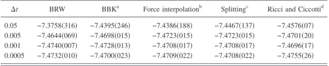
Many discretization schemes exist for Langevin dynam-ics. In order to choose which algorithm is best for VMC, we have tested four different schemes available in the literature,13–16 with parameters = 1, ␥= 1, and m = 1. Our benchmark system is a lithium atom, and a single determi-nantal wave function built upon Slater-type atomic orbitals, multiplied by a Jastrow factor. We turn off the accept/reject step in these preliminary tests, since our purpose is to com-pare the time-step errors for the various algorithms. From the results displayed in Table I, one can see that the Ricci-Ciccotti algorithm16is the method which generates the small-est time-step error. This algorithm reads
Rn+1= Rn+共⌬t/m兲Pne−␥⌬t/2+共⌬t/2m兲 ⫻关− ⵜV共Rn兲⌬t + Gn兴e−␥⌬t/4 , 共19兲 Pn+1= Pne−␥⌬t−共⌬t/2兲关ⵜV共Rn兲 +ⵜV共Rn+1兲兴e−␥⌬t/2+ Gne−␥⌬t/2,
where Gn are iid. Gaussian random vectors with zero mean
and variance2I3Nwith2=共2␥m /兲⌬t.
It can be seen from TableIthat the Ricci-Ciccotti algo-rithm also outperforms the biased random walk 共12兲, as far as sampling issues are concerned. In the following, we shall therefore use the Ricci-Ciccotti algorithm.
3. Metropolized Langevin dynamics
The discretized Langevin dynamics does not exactly sample the target distribution ⌸, but rather from some ap-proximation⌸⌬tof⌸. It is therefore tempting to introduce a Metropolis-Hastings accept/reject step to further improve the quality of the sampling. Unfortunately, this idea cannot be straightforwardly implemented for two reasons.
• First, this is not technically feasible, since the Markov chain defined by共19兲does not have a transition density. Indeed, as the same Gaussian random vectors Gn are
used to update both the positions and the momenta, the measure p共共Rn, Pn兲, ·兲 is supported on a 3N-dimensional submanifold of the phase space R3N
⫻R3N.
• Second, leaving apart the above mentioned technical difficulty, which is specific to the Ricci-Ciccotti scheme, the Langevin dynamics is a priori not an effi-cient Markov chain for the Metropolis-Hastings
algo-rithm because it does not satisfy the detailed balance property.
Let us now explain how to tackle these two issues, start-ing with the first one.
To make it compatible with the Metropolis-Hastings framework, one needs to slightly modify the Ricci-Ciccotti algorithm. Following 共Refs. 14 and17兲, we thus introduce iid correlated Gaussian vectors 共G1,in , G2,in 兲 共1艋i艋3N兲 such that 具共G1,i n 兲2典 = 1 2= ⌬t m␥
冉
2 − 3 − 4e−␥⌬t+ e−2␥⌬t ␥⌬t冊
, 共20a兲 具共G2,i n 兲2典 = 2 2=m 共1 − e−2␥⌬t兲, 共20b兲 具G1,i n G2,in 典 12 = c12= 共1 − e−␥⌬t兲2 ␥12 . 共20c兲Setting G1n=共G1,in 兲1艋i艋3N and G2n=共G2,in 兲1艋i艋3N, the modified Ricci-Ciccotti algorithm reads
Rn+1= Rn+共⌬t/m兲Pne−␥⌬t/2 −共⌬t2/2m兲 ⵜ V共Rn兲e−␥⌬t/4+ G1 n , 共21兲 Pn+1= Pne−␥⌬t−共⌬t/2兲关ⵜV共Rn兲 +ⵜV共Rn+1兲兴e−␥⌬t/2+ G2 n .
The above scheme is a consistent discretization of 共14兲and the corresponding Markov chain does have a transition den-sity, which reads共see Appendix兲
T⌬tMRC共共Rn,Pn兲 → 共Rn+1,Pn+1兲兲 = Z−1exp
冋
− 1 2共1 − c122 兲冉冉
兩d1兩 1冊
2 +冉
兩d2兩 2冊
2 − 2c12 d1 1 ·d2 2冊
册
, 共22a兲 with d1= Rn+1− Rn−⌬t Pn me −␥⌬t/2+⌬t2 2mⵜ V共R n兲e−␥⌬t/4 , 共22b兲TABLE I. Comparison of different discretization schemes for Langevin dynamics. The reference energy is −7.471 98共4兲 a.u..
⌬t BRW BBKa Force interpolationb Splittingc Ricci and Ciccottid 0.05 −7.3758共316兲 −7.4395共246兲 −7.4386共188兲 −7.4467共137兲 −7.4576共07兲 0.005 −7.4644共069兲 −7.4698共015兲 −7.4723共015兲 −7.4723共015兲 −7.4701共20兲 0.001 −7.4740共007兲 −7.4728共013兲 −7.4708共017兲 −7.4708共017兲 −7.4696共17兲 0.0005 −7.4732共010兲 −7.4700共023兲 −7.4709共022兲 −7.4708共022兲 −7.4755共26兲 aReference13. bReference14. cReference15. dReference16.
d2= Pn+1− Pne−␥⌬t+1
2⌬t关ⵜV共R
n兲 + ⵜV共Rn+1兲兴e−␥⌬t/2.
共22c兲 Unfortunately, inserting directly the transition density共22兲 in the Metropolis-Hastings algorithm leads to a high rejection rate. Indeed, if共Rn, Pn兲 and 共Rn+1, Pn+1兲 are related through 共21兲, T⌬tMRC共共Rn, Pn兲→共Rn+1, Pn+1兲兲 usually is much greater than T⌬tMRC共共Rn+1, Pn+1兲→共Rn, Pn兲兲, since the probability that the random forces are strong enough to make the particle go back in one step from where it comes is very low in general. This is related to the fact that the Langevin dynamics does not satisfy the detailed balance relation.
It is, however, possible to further modify the overall al-gorithm by ensuring some microscopic reversibility in order to finally obtain low rejection rates. For this purpose, we introduce momentum reversions. Denoting by T⌬tLangevin the transition density of the Markov chain obtained by integrat-ing共14兲exactly on the time interval关t,t+⌬t兴, it is indeed not
difficult to check 共under convenient assumptions on V= −ln兩⌿兩2兲 that the Markov chain defined by the transition
den-sity T ˜ ⌬t Langevin共共R,P兲 → 共R
⬘
,P⬘
兲兲 = T⌬tLangevin共共R,P兲 → 共R⬘
,− P⬘
兲兲 共23兲 is ergodic with respect to⌸ and satisfies the detailed balance property,⌸共R,P兲T˜⌬tLangevin共共R,P兲 → 共R
⬘
,P
⬘
兲兲=⌸共R
⬘
,P⬘
兲T˜⌬tLangevin共共R⬘
,P⬘
兲→ 共R,P兲兲. 共24兲 Replacing the exact transition density T⌬tLangevin by the ap-proximation T⌬tMRC, we now consider the transition density
T ˜ ⌬t MRC共共R,P兲 → 共R
⬘
,P⬘
兲兲 = T⌬tMRC共共R,P兲 → 共R⬘
,− P⬘
兲兲. 共25兲 The new sampling algorithm that we propose can be stated as follows.• Propose a move from共Rn, Pn兲 to 共R˜n+1, P˜n+1兲 using the
transition density T˜⌬tMRC. In other words, perform one step of the modified Ricci-Ciccotti algorithm,
R*n+1= Rn+共⌬t/m兲Pne−␥⌬t/2 −共⌬t2/2m兲 ⵜ V共Rn兲e−␥⌬t/4+ G1n, 共26兲 P*n+1= Pne−␥⌬t−共⌬t/2兲关ⵜV共Rn兲 +ⵜV共Rn+1兲兴e−␥⌬t/2+ G2n, and set共R˜n+1, P˜n+1兲=共R * n+1, −P * n+1兲.
• Compute the acceptance rate,
A共共Rn,Pn兲 → 共R˜n+1,P˜n+1兲兲 = min
冉
⌸共R˜ n+1,P˜n+1兲T˜ ⌬t MRC共共R˜n+1,P˜n+1兲 → 共Rn ,Pn兲兲 ⌸共Rn ,Pn兲T˜⌬tMRC共共Rn,Pn兲 → 共R˜n+1,P˜n+1兲兲 ,1冊
.• Draw a random variable Ununiformly distributed in共0, 1兲 and if Un艋A共共Rn
, Pn兲→共R˜n+1, P˜n+1兲兲, accept the proposal: 共R¯n+1, P¯n+1兲=共R˜n+1, P˜n+1兲, and if Un
⬎A共共Rn, Pn兲→共R˜n+1, P˜n+1兲兲, reject the proposal, and
set共R¯n+1, P¯n+1兲=共Rn, Pn兲.
• Reverse the momenta,
共Rn+1,Pn+1兲 = 共R¯n+1,− P¯n+1兲. 共27兲
Note that a momentum reversion is systematically per-formed just after the Metropolis-Hastings step. As the invari-ant measure⌸ is left unchanged by this operation, the global algorithm 共Metropolis-Hastings step based on the transition density T˜⌬tMRCplus momentum reversion兲 actually samples ⌸. The role of the final momentum reversion is to preserve the underlying Langevin dynamics: while the proposals are ac-cepted, the above algorithm generates Langevin trajectories, that are known to efficiently sample an approximation of the target density⌸. Numerical tests seem to show that, in ad-dition, the momentum reversion also plays a role when the
proposal is rejected: it seems to increase the acceptance rate of the next step, preventing the walkers from being trapped in the vicinity of the nodal surface⌿−1共0兲.
As the points共Rn, Pn兲 of the phase space generated by the above algorithm form a sampling of⌸, the positions 共Rn兲 sample兩⌿共R兲兩2/兰R3N兩⌿兩2and can therefore be used for VMC calculations.
III. NUMERICAL EXPERIMENTS AND APPLICATIONS A. Measuring the efficiency
A major drawback of samplers based on Markov pro-cesses is that they generate sequentially correlated data. For a trajectory of L steps, the effective number of independent observations is in fact Leff= L / Ncorr, where Ncorris the
corre-lation length, namely, the number of successive correlated
moves.
In the following applications, we provide estimators for the correlation length Ncorrand for the so-called inefficiency
共see below兲, which are relevant indicators of the quality of the sampling. In this section, following Stedman et al.,18we describe the way these quantities are defined and computed.
The sequence of samples is split into NB blocks of LB
steps, where the number LB is chosen such that it is a few
orders of magnitude higher than Ncorr. The mean energy is
具EL典兩⌿兩2 and the variance is 2=具共EL−具EL典兩⌿兩2兲2典兩⌿兩2. These quantities are defined independently on the VMC algorithm used. The empirical mean of the local energy reads
具EL典兩⌿兩2 NB,LB= 1
NBLB
兺
i=1 NBLBEL共Ri兲. 共28兲
The empirical variance over all the individual steps is given by 关NB,LB兴2= 1 NBLB
兺
i=1 NBLB 共EL共Ri兲 − 具EL典兩⌿兩2 NB,LB兲2, 共29兲and the empirical variance over the blocks by 关B
NB,LB兴2= 1
NB
兺
i=1 NB共EB,i−具EL典兩⌿兩2
NB,LB兲2, 共30兲
where EB,i is the average energy over block i,
EB,i= 1
LBj=共i−1兲L
兺
B+1 iLBEL共Rj兲. 共31兲
Following Ref.18, we define the correlation length as
Ncorr= lim NB→⬁ lim LB→⬁ LB 关B NB,LB兴2 关NB,LB兴2, 共32兲
and the inefficiencyof the run as
= lim NB→⬁ lim LB→⬁ LB关B NB,LB兴2. 共33兲
On the numerical examples presented below, the relative fluctuations of the quantities LB关B
NB,LB兴2/关NB,LB兴2 and
LB关B
NB,LB兴2become small for L
B⬎50 and NB⬎50.
The definition of these two quantities can be understood as follows. Since LBⰇNcorr and only LB/ Ncorr are
indepen-dent samples among the samples in the block, the central limit theorem yields EB,i⯝具EL典兩⌿兩2+Gi/
冑
LB/ Ncorr, whereGi are iid normal random variables. Thus, in the limit NB
→⬁ and LB→⬁, we obtain that 共B
NB,LB兲2=2/共L
B/ Ncorr兲.
Since limNB→⬁limLB→⬁关NB,LB兴2=2, we obtain共32兲. The
in-efficiency is thus equal to Ncorr2 and is large if the
vari-ance is large, or if the number of correlated steps is large. Using this measure of efficiency, we can now compare the sampling algorithms共the simple random walk, the biased random walk, and the Langevin algorithm兲 for various sys-tems. In any case, a Metropolis-Hastings accept/reject step is used. We found empirically from several tests that conve-nient values for the parameters of the Langevin algorithm are
␥= 1 and m = Z3/2, where Z is the highest nuclear charge
among all the nuclei. For each algorithm, we compare the efficiency for various values of the step length, namely, the increment⌬R in the case of the simple random walk, and the time step ⌬t for the other two schemes. For a given algo-rithm, simple arguments corroborated by numerical tests show that there exists an optimal value of this increment: for smaller 共respectively for larger兲 increments, the correlation
between two successive positions increases since the dis-placement of the particle is small 共respectively since many moves are rejected兲, and this increases the number of corre-lated steps Ncorr.
One can notice on the results 共see Tables II–V兲 that a large error bar corresponds to large values for Ncorr and.
The quantities Ncorrandare a way to refine the measure of
efficiency, since the same length of error bar may be ob-tained for different values of the numerical parameters.
Let us now present some numerical tests. We compare the algorithms and parameters at a fixed computational cost. The reference values are obtained by ten times longer VMC simulations. The error bars given in parentheses are 68% confidence intervals. We also provide the mean acceptance rate 共denoted by 具A典 in the tables兲 and, when it is relevant, the mean of the length of the increment Rn+1− Rn over one
time step 共denoted by 具兩⌬R兩典 in the tables兲 for the biased random walk and the Langevin dynamics. These tests were performed using the QMC=Chem program,19 and the wave functions are available upon request.
B. Atoms
Lithium. The lithium atom was chosen as a first simple
example. The wave function is the same as for the bench-mark system used for the comparison of the various Lange-vin schemes, namely, a single Slater determinant of
Slater-TABLE II. The lithium atom: comparison of the simple random walk, the biased random walk, and the proposed Langevin algorithm. The runs were carried out with 100 walkers, each realizing 50 blocks of 1000 steps. The reference energy is −7.471 98共4兲 a.u.
⌬R 具EL典 Ncorr 具A典
Simple random walk
0.05 −7.471 26共183兲 94.5± 3.3 11.72共42兲 0.91 0.10 −7.472 39共97兲 35.2± 1.2 4.8共14兲 0.82 0.15 −7.471 89共75兲 20.5共5兲 2.30共06兲 0.74 0.20 −7.471 57共56兲 14.3共4兲 1.62共04兲 0.66 0.25 −7.471 82共56兲 12.1共3兲 1.40共05兲 0.59 0.30 −7.471 89共56兲 11.4共3兲 1.57共17兲 0.52 0.35 −7.472 75共59兲 12.4共3兲 1.57共17兲 0.46 0.40 −7.471 30共63兲 14.4共5兲 1.93共22兲 0.40
⌬t 具EL典 Ncorr 具兩⌬R兩典 具A典
Biased random walk
0.01 −7.471 98共53兲 10.31共29兲 1.23共3兲 0.284共09兲 0.98 0.03 −7.471 56共39兲 5.26共14兲 0.73共7兲 0.444共21兲 0.92 0.04 −7.471 95共35兲 4.82共12兲 0.57共3兲 0.486共26兲 0.88 0.05 −7.472 19共32兲 4.74共11兲 0.55共2兲 0.514共31兲 0.85 0.06 −7.472 04共38兲 4.95共11兲 0.58共3兲 0.533共36兲 0.81 0.07 −7.472 51共32兲 5.39共14兲 0.61共3兲 0.546共40兲 0.78 0.10 −7.472 49共42兲 7.56共25兲 0.87共5兲 0.555共50兲 0.68 Langevin 0.20 −7.472 33共34兲 5.07共10兲 0.60共1兲 0.236共08兲 0.97 0.30 −7.472 07共34兲 4.14共09兲 0.47共1兲 0.328共15兲 0.93 0.35 −7.471 80共31兲 3.96共08兲 0.45共1兲 0.366共18兲 0.91 0.40 −7.471 85共29兲 3.75共08兲 0.44共2兲 0.399共22兲 0.89 0.45 −7.472 64共29兲 3.88共08兲 0.45共2兲 0.426共25兲 0.86 0.50 −7.471 91共29兲 4.07共14兲 0.46共2兲 0.426共25兲 0.84 0.60 −7.472 58共32兲 4.78共16兲 0.52共2兲 0.481共36兲 0.78
type basis functions improved by a Jastrow factor to take account of the electron correlation. The reference energy as-sociated with this wave function is −7.471 98共4兲 a.u., and the comparison of the algorithms is given in TableII. The runs were made of 100 random walks composed of 50 blocks of 1000 steps. For the simple random walk, the lowest values of the correlation length and of the inefficiency are, respec-tively, 11.4 and 1.40. The biased random walk is much more efficient, since the optimal correlation length and ineffi-ciency are more than twice smaller, i.e., 4.74 and 0.55. The proposed algorithm is even more efficient: the optimal cor-relation length is 3.75 and the optimal inefficiency is 0.44.
Fluorine. The fluorine atom was chosen for its relatively
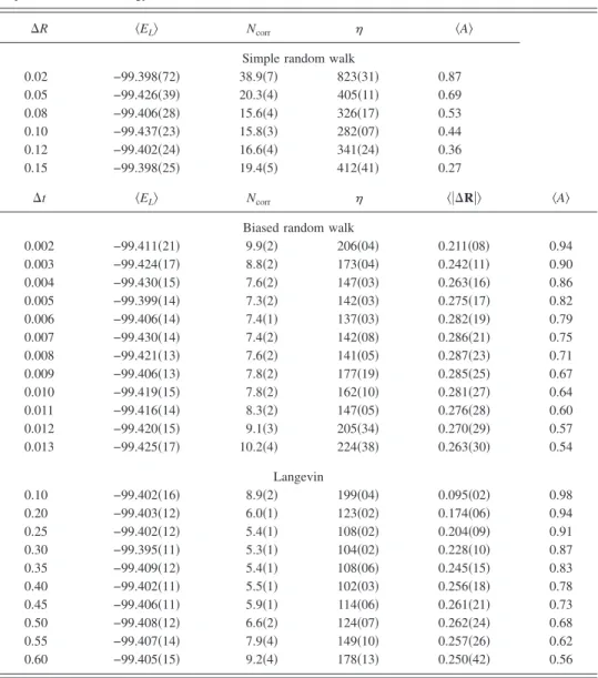
“high” nuclear charge共Z=9兲, leading to a time scale separa-tion of the core and valence electrons. The wave funcsepara-tion is a Slater determinant with Gaussian-type basis functions where the 1s orbital was substituted by a Slater-type orbital, with a reference energy of −99.397共2兲 a.u. The runs were made of 100 random walks composed of 100 blocks of 100 steps. The results are given in Table III. For the simple
random walk, the lowest values of the correlation length and of the inefficiency are, respectively, 15.6 and 282. The biased random walk, for which the optimal correlation length and inefficiency are 7.4 and 137 respectively, is again twice more efficient than the simple random walk. The Langevin algo-rithm is more efficient than the biased random walk: the optimal correlation length is 5.3 and the optimal inefficiency is 102.
Copper. We can go even further in the time scale
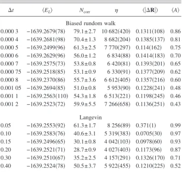
sepa-ration and take the copper atom 共Z=29兲 as an example. The wave function is a Slater determinant with a basis of Slater-type atomic orbitals, improved by a Jastrow factor to take account of the electron correlation. The reference energy is −1639.2539共24兲. The runs were made of 40 random walks composed of 500 blocks of 500 steps. From Table IV, one can remark that the Langevin algorithm is again more effi-cient than the biased random walk, since the optimal corre-lation length and inefficiency are, respectively, 28.7 and 4027, whereas using the biased random walk, these values are 51.0 and 5953.
TABLE III. The fluorine atom: comparison of the simple random walk, the biased random walk, and the proposed Langevin algorithm. The runs were carried out with 100 walkers, each realizing 100 blocks of 100 steps. The reference energy is −99.397共2兲 a.u.
⌬R 具EL典 Ncorr 具A典
Simple random walk
0.02 −99.398共72兲 38.9共7兲 823共31兲 0.87 0.05 −99.426共39兲 20.3共4兲 405共11兲 0.69 0.08 −99.406共28兲 15.6共4兲 326共17兲 0.53 0.10 −99.437共23兲 15.8共3兲 282共07兲 0.44 0.12 −99.402共24兲 16.6共4兲 341共24兲 0.36 0.15 −99.398共25兲 19.4共5兲 412共41兲 0.27
⌬t 具EL典 Ncorr 具兩⌬R兩典 具A典
Biased random walk
0.002 −99.411共21兲 9.9共2兲 206共04兲 0.211共08兲 0.94 0.003 −99.424共17兲 8.8共2兲 173共04兲 0.242共11兲 0.90 0.004 −99.430共15兲 7.6共2兲 147共03兲 0.263共16兲 0.86 0.005 −99.399共14兲 7.3共2兲 142共03兲 0.275共17兲 0.82 0.006 −99.406共14兲 7.4共1兲 137共03兲 0.282共19兲 0.79 0.007 −99.430共14兲 7.4共2兲 142共08兲 0.286共21兲 0.75 0.008 −99.421共13兲 7.6共2兲 141共05兲 0.287共23兲 0.71 0.009 −99.406共13兲 7.8共2兲 177共19兲 0.285共25兲 0.67 0.010 −99.419共15兲 7.8共2兲 162共10兲 0.281共27兲 0.64 0.011 −99.416共14兲 8.3共2兲 147共05兲 0.276共28兲 0.60 0.012 −99.420共15兲 9.1共3兲 205共34兲 0.270共29兲 0.57 0.013 −99.425共17兲 10.2共4兲 224共38兲 0.263共30兲 0.54 Langevin 0.10 −99.402共16兲 8.9共2兲 199共04兲 0.095共02兲 0.98 0.20 −99.403共12兲 6.0共1兲 123共02兲 0.174共06兲 0.94 0.25 −99.402共12兲 5.4共1兲 108共02兲 0.204共09兲 0.91 0.30 −99.395共11兲 5.3共1兲 104共02兲 0.228共10兲 0.87 0.35 −99.409共12兲 5.4共1兲 108共06兲 0.245共15兲 0.83 0.40 −99.402共11兲 5.5共1兲 102共03兲 0.256共18兲 0.78 0.45 −99.406共11兲 5.9共1兲 114共06兲 0.261共21兲 0.73 0.50 −99.408共12兲 6.6共2兲 124共07兲 0.262共24兲 0.68 0.55 −99.407共14兲 7.9共4兲 149共10兲 0.257共26兲 0.62 0.60 −99.405共15兲 9.2共4兲 178共13兲 0.250共42兲 0.56
C. The phenol molecule
The phenol molecule was chosen to test the proposed algorithm because it contains three different types of atoms 共H, C, and O兲. The wave function here is a single Slater determinant with Gaussian-type basis functions. The core molecular orbitals of the oxygen and carbon atoms were sub-stituted by the corresponding atomic 1s orbitals. The com-parison of the biased random walk with the Langevin algo-rithm is given in Table V. The optimal correlation length using the biased random walk is 10.17, whereas it is 8.23 with our Langevin algorithm. The optimal inefficiency is again lower with the Langevin algorithm共544兲 than with the biased random walk共653兲.
D. Discussion of the results
We observe that on our numerical tests, the Langevin dynamics is always more efficient than the biased random walk. Indeed, we notice the following.
• The error bar共or Ncorr, or兲 obtained with the Langevin dynamics for an optimal set of numerical parameters is always smaller than the error bar obtained with other algorithms 共for which we also optimize the numerical parameters兲.
• The size of the error bar does not seem to be as sensi-tive to the choice of the numerical parameters as for other methods. In particular, we observe on our numeri-cal tests that the value⌬t=0.2 seems to be convenient to obtain good results with the Langevin dynamics, whatever the atom or molecule.
ACKNOWLEDGMENT
This work was supported by the ACI “Molecular Simu-lation” of the French Ministry of Research.
APPENDIX: DERIVATION OF THE TRANSITION PROBABILITY„22…
The random vector共d1, d2兲 关defined by共22b兲and共22c兲兴 is a Gaussian random vector and therefore admits a density with respect to the Lebesgue measure in R6N. If, for 1艋i
艋3N, we denote by d1,i and d2,i the components of d1 and
d2, we observe that the Gaussian random vectors 共d1,i, d2,i兲 are iid. Therefore, the transition probability T共共Rn, Pn兲
→共Rn+1, Pn+1兲兲 reads
T共共Rn,Pn兲 → 共Rn+1,Pn+1兲兲 = Z−1共p共d1,i,d2,i兲兲3N, 共A1兲
where Z is a normalization constant and p denotes the den-sity共in R2兲 of the Gaussian random vectors 共d
1,i, d2,i兲.
From Eq.共21兲, one can see that
d1,i= Rin+1− Ri n −⌬tPi n me −␥⌬t/2+⌬t2 2mⵜiV共R n兲e−␥⌬t/4 , d2,i= Pi n+1 − Pi n e−␥⌬t+1 2⌬t关ⵜiV共R n兲 + ⵜ iV共Rn+1兲兴e−␥⌬t/2
is a Gaussian random vector with covariance matrix ⌫ =
冋
1 2 c 1212 c1212 2 2册
. Thus p共d1,d2兲 = 共2冑
det⌫兲−1exp冉
− 1 2共d1,d2兲⌫ −1共d 1,d2兲T冊
. 共A2兲 Since ⌫−1= 1 共1 − c12 2 兲冋
1/12 − c12/12 − c12/12 1/2 2册
,共22c兲is easily obtained from共A1兲and共A2兲.
TABLE IV. The copper atom: comparison of the biased random walk with the proposed Langevin algorithm. The runs were carried out with 40 walk-ers, each realizing 500 blocks of 500 steps. The reference energy is −1639.2539共24兲 a.u.
⌬t 具EL典 Ncorr 具兩⌬R兩典 具A典
Biased rundom walk
0.000 3 −1639.2679共78兲 79.1± 2.7 10 682共420兲 0.1311共108兲 0.86 0.000 4 −1639.2681共98兲 70.4± 1.3 8 682共204兲 0.1385共137兲 0.81 0.000 5 −1639.2499共96兲 61.3± 2.5 7 770共297兲 0.114共162兲 0.75 0.000 6 −1639.2629共96兲 56.0± 1.2 6 834共88兲 0.1414共183兲 0.70 0.000 7 −1639.2575共73兲 53.8± 0.8 6 420共81兲 0.1393共201兲 0.65 0.000 75 −1639.2518共85兲 53.1± 0.9 6 330共91兲 0.1377共209兲 0.62 0.000 8 −1639.2370共86兲 55.7± 3.6 6 612共405兲 0.1357共216兲 0.60 0.001 05 −1639.2694共85兲 51.0± 0.8 5 953共90兲 0.1228共241兲 0.48 0.001 1 −1639.2563共110兲 54.3±1.8 6 513共221兲 0.1198共245兲 0.46 0.001 2 −1639.2523共72兲 59.9± 5.5 7 266共658兲 0.1136共251兲 0.43 Langevin 0.05 −1639.2553共92兲 61.3± 1.7 8 256共89兲 0.371共1兲 0.99 0.10 −1639.2583共76兲 40.6± 3.1 5 319共383兲 0.0705共30兲 0.97 0.15 −1639.2496共65兲 30.1± 0.8 4 042共103兲 0.0978共60兲 0.93 0.20 −1639.2521共71兲 28.7± 0.9 4 027共403兲 0.1173共96兲 0.87 0.30 −1639.2510共67兲 35.2± 2.5 4 157共291兲 0.1326共170兲 0.71 0.40 −1639.2524共78兲 50.5± 3.7 5 922共455兲 0.1210共225兲 0.52
TABLE V. The phenol molecule: comparison of the biased random walk with the proposed Langevin algorithm. the runs were carried out with 100 walkers, each realizing 100 blocks of 100 steps. The reference energy is −305.647共2兲 a.u.
⌬t 具EL典 Ncorr 具兩⌬R兩典 具A典
Biased random walk
0.003 −305.6308共83兲 18.71共24兲 1368共12兲 0.522共29兲 0.85 0.004 −305.6471共78兲 16.00共28兲 1193共30兲 0.547共36兲 0.80 0.005 −305.6457共65兲 15.29共20兲 1077共14兲 0.555共43兲 0.74 0.006 −305.6412共79兲 15.00共17兲 1018共11兲 0.552共48兲 0.69 0.007 −305.6391共67兲 14.52共26兲 1051共53兲 0.540共52兲 0.63 0.008 −305.6530共65兲 14.72共19兲 980共10兲 0.523共56兲 0.58 0.009 −305.6555共82兲 15.28共28兲 1272共163兲 0.502共59兲 0.54 Langevin 0.05 −305.6417共101兲 23.13共41兲 1932共41兲 0.126共02兲 0.99 0.1 −305.6416共68兲 13.97共22兲 1189共23兲 0.240共06兲 0.97 0.2 −305.6496共57兲 9.70共13兲 812共12兲 0.408共20兲 0.89 0.3 −305.6493共56兲 9.36共16兲 817共36兲 0.487共36兲 0.78 0.4 −305.6473共58兲 12.21共22兲 834共20兲 0.485共50兲 0.61 0.5 −305.6497共80兲 17.51共44兲 1237共52兲 0.425共58兲 0.43
1D. Bressanini and P. J. Reynolds, Advances in Chemical Physics共Wiley, New York, 1999兲, Vol. 105, p. 37.
2E. Cancès, F. Legoll, and G. Stoltz, IMA Report No. 2040, 2005 共unpub-lished兲; http://www.ima.umn.edu/preprints/apr2005/2040.pdf
3M. Caffarel and P. Claverie, J. Chem. Phys. 88, 1100共1988兲.
4C. J. Umrigar, M. P. Nightingale, and K. J. Runge, J. Chem. Phys. 99, 2865共1993兲.
5N. Metropolis, A. W. Rosenbluth, M. N. Rosenbluth, A. M. Teller, and E. J. Teller, J. Chem. Phys. 21, 1087共1953兲.
6W. K. Hastings, Biometrika 57, 97共1970兲.
7S. P. Meyn and R. L. Tweedie, Markov Chains and Stochastic Stability 共Springer, Berlin, 1993兲.
8D. Ceperley, G. V. Chester, and M. H. Kalos, Phys. Rev. B 16, 3081 共1977兲.
9E. Cancès, B. Jourdain, and T. Lelièvre, Math. Models Meth. Appl. Sci. 16, 1403共2006兲.
10C. J. Umrigar, Phys. Rev. Lett. 71, 408共1993兲.
11Z. Sun, M. M. Soto, and W. A. Lester, Jr., J. Chem. Phys. 100, 1278 共1994兲.
12D. Bressanini and P. J. Reynolds, J. Chem. Phys. 111, 6180共1999兲. 13B. Brünger, C. L. Brooks, and M. Karplus, Chem. Phys. Lett. 105, 495
共1984兲.
14M. P. Allen and D. J. Tildesley, Computer Simulation of Liquids共Oxford University Press, Oxford, 1989兲 and references in Sec. 9.3.
15J. A. Izaguirre, D. P. Catarello, J. M. Wozniak, and R. D. Skeel, J. Chem. Phys. 114, 2090共2001兲.
16A. Ricci and G. Ciccotti, Mol. Phys. 101, 1927共2003兲. 17S. Chandrasekhar, Rev. Mod. Phys. 15, 1共1943兲.
18N. L. Stedman, W. M. C. Foulkes, and M. Nekovee, J. Chem. Phys. 109, 2630共1998兲.
19M. Caffarel, QMC= Chem is a quantum Monte Carlo program, IRSAMC, Université Paul Sabatier-CNRS, Toulouse, France.